Effects of density stratification on the frequencies of the inertial-gravity modes of the Earth's fluid core

Seyed-Mahmoud, B.; Moradi, A.; Kamruzzaman, M.; Naseri, H.

doi:10.1093/gji/ggv215

Abstract

The Earth's outer core is a rotating ellipsoidal shell of compressible, stratified and self-gravitating fluid. As such, in the treatment of geophysical problems a realistic model of this body needs to be considered. In this work, we consider compressible and stratified fluid core models with different stratification parameters, related to the local Brunt-Väisälä frequency, in order to study the effects of the core's density stratification on the frequencies of some of the inertial-gravity modes of this body. The inertial-gravity modes of the core are free oscillations with periods longer than 12 hr. Historically, an incompressible and homogeneous fluid is considered to study these modes and analytical solutions are known for the frequencies and the displacement eigenfunctions of a spherical model. We show that for a compressible and stratified spherical core model the effects of non-neutral density stratification may be significant, and the frequencies of these modes may change from model to model. For example, for a spherical core model the frequency of the spin-over mode, the (2, 1, 1) mode, is unaffected while that of the (4, 1, 1) mode is changed from −0.410 for the Poincaré core model to −0.434, −0.447 and −0.483 for core models with the stability parameter β = −0.001, −0.002 and −0.005, respectively, a maximum change of about 18 per cent when β = −0.005. Our results also show that for small stratification parameter, |β| ≤ 0.005, the frequency of an inertial-gravity mode is a nearly linear function of β but the slope of the line is different for different modes, and that the effects of density stratification on the frequency of a mode is likely related to its spatial structure, which remains the same in different Earth models. We also compute the frequencies of some of the modes of the ‘PREM’ (spherical shell) core model and show that the frequencies of these modes may also be significantly affected by non-zero β.

Numerical solutions, Core, outer core and inner core, Planetary interiors

1 INTRODUCTION

The innermost region of the Earth consists of a liquid outer core and a solid inner core. The radius of the inner core is estimated to be 1221.5 km and that of the outer core 3480 km for the `PREM' Earth model (Dziewonski & Anderson 1981). The fluid core plays a key role in many geophysical studies. For example, a perfectly rigid body with the same mass distribution as that of the Earth is expected to have a free Eulerian wobble with period of about 306 days; all periods in this paper are in sidereal days. The presence of the liquid core changes this period to about 270 days and gives rise to an additional retrograde wobble of nearly diurnal period, corresponding to a nutation of about 350 days. Once elasticity and the presence of oceans are taken into account, the Eulerian wobble period is about 435 days (the Chandler wobble) and the free core nutation period about 460 days, assuming that the steadily rotating configuration is one of hydrostatic equilibrium.

Since the core is not directly accessible, much is still unknown about its properties. The distributions of material properties such as the density ρ and Lamé parameter λ in the core are established through theoretical and observational studies using ray seismology and free oscillations. However, the stability parameter β (Pekeris & Accad 1972), which is directly related to the density stratification (see eq. 8 below) in the core, is found from the density gradient which is less precisely constrained than the density itself as determined from the seismic free oscillations (Masters 1979), and has an approximate limit of |β| ≤ 0.03–0.05 in the core (see also Wu & Rochester 1990). For a detailed discussion of the influence of β on the frequencies of the Earth's rotational modes, which include both wobble modes and the inertia-gravity modes (see Rogister & Valette 2009).

The spectrum of free oscillations possible in the liquid core includes the inertial waves if the core is incompressible or neutrally stratified, or inertial-gravity modes if it is the stratification deviates from neutral. The inertial modes depend solely on the Coriolis force but the inertial-gravity modes have this force and the radial component of gravitational force as their restoring forces (Friedlander 1985). Among the first who studied these modes were Hough (1895), Bryan (1889) and Poincaré (1910). The core model they considered was a rotating inviscid and homogeneous fluid ellipsoid with a rigid boundary. Their works yielded analytical solutions (Greenspan 1969) for the eigenfrequencies and eigenfunctions of the inertial modes of the model. Kudlick (1966) (see also Greenspan 1969) considered viscosity in the above model and found analytical expressions for the solution of the inertial modes. Rogister & Valette (2009) investigate the effects of non-neutral density stratification on the rotational modes through the square of the Brunt-Väisälä frequency N². They agree that a highly truncated system of spherical harmonics is not adequate to fully describe the rotational modes hence label the modes they computed pseudo-modes. They show that for a highly tuned value of a constant buoyancy parameter N² (see eq. 9), these modes may interact with at least three of the Earth's wobble and nutation modes: the Chandler Wobble, the Free Inner Core Nutation and the Free Core Nutation modes.

The Poincaré problem, which describes the inertial modes of a homogeneous and incompressible fluid, is a hyperbolic equation subject to boundary condition, a condition which makes the problem ill-posed (Aldridge 1967; Stewartson & Rickard 1969)[see also section 6 of Swart et al. (2007)]. The existence of the analytical solutions then depends on the geometry of the container. These solutions do not exist in a thick spherical (or spheroidal) shell, which is the approximate geometry of the Earth's fluid core. Rieutord & Valdettaro (1997) (see also Rieutord 1995) studied the inertial modes of an incompressible and homogeneous fluid shell of small viscosity and infer that with the exception of a set of special cases for which analytical solutions exist (Stewartson & Rickard 1969), no solutions exist for the inertial modes of an incompressible fluid shell in the asymptotic limit of zero viscosity. Seyed-Mahmoud & Rochester (2006) and Seyed-Mahmoud et al. (2007) considered a compressible and neutrally stratified fluid to study the inertial modes of rotating and self-gravitating fluid of spherical and spherical shell geometries. Their results show that for a spherical geometry, to the degree they investigated, the frequencies of the inertial modes of a neutrally stratified fluid are almost identical to those of the Poincaré model.

In this work, we investigate the influence of non-zero β on the frequencies of these modes using several spherical core models based on PREM, but modified so that the stratification parameter varies in a systematic way about β = 0. We show that for small β the frequency of a mode is a linear function of β but the slope of the line depends on the spatial structure of the mode. We also compute some of the inertial-gravity modes of the `PREM' core model

2 GOVERNING EQUATIONS

Seyed-Mahmoud & Rochester (2006) show that the dynamics of the Earth's fluid core may be described by three equations in terms of three scalar potentials |$\chi = \frac{p_1}{\rho _0}$|⁠, ζ = ∇ · u and V₁ :

\begin{equation} {\nabla }^2 V_1-4 \pi G \rho _0 \left\lbrace \beta \zeta -\frac{1-\beta }{\alpha ^2} \chi \right\rbrace =0 , \end{equation}

(1)

\begin{equation} {{\nabla }}\cdot \lbrace {\bf \tilde{\Gamma }}_{\bf p}\cdot {{{\nabla }}(\chi -V_1)}-\beta {{\bf C}}^*\zeta \rbrace -\omega ^2(\omega ^2-4 \Omega ^2)\zeta =0 , \end{equation}

(2)

\begin{equation} {{\bf C}}\cdot {{{\nabla }}(\chi -V_1)}-\omega ^2(\omega ^2-4 \Omega ^2)\chi -B\zeta =0, \end{equation}

(3)

where u, ρ₀ and p₀ are the Lagrangian displacement, the equilibrium density and pressure, respectively; ρ₁, p₁ and V₁ are the Eulerian perturbations in density, pressure and gravitational potential, respectively; G is the gravitational constant, g₀ the gravity, β the stability parameter, α the local speed of compressional waves, ω the frequency of a mode, and

\begin{equation} {\bf \tilde{\Gamma }}_{\bf p}=\omega ^2 \tilde{{\bf 1}}-4\Omega ^2 {{\bf e}_3}{{\bf e}_3}+2 i \omega \Omega {{\bf e}_3} \times \tilde{{\bf 1}} , \end{equation}

(4)

\begin{equation} B=\alpha ^2 \omega ^2(\omega ^2-4 \Omega ^2)+\beta \left[\omega ^2 g_0^2 -4\Omega ^2 ({{\bf e}_3}\cdot {{\bf g}_0)}^2 \right] , \end{equation}

(5)

\begin{equation} {{\bf C}}= -\omega ^2{{\bf g}}_0 +4\Omega ^2{{\bf e}_3}\cdot {{\bf g}}_0{{\bf e}_3} +2 i \omega \Omega {{\bf e}_3} \times {\bf g}_0 \end{equation}

(6)

with C^* being the complex conjugate of C. The displacement vector is given as

\begin{equation} \omega ^2(\omega ^2-4\Omega ^2){{\bf u}}={\bf \tilde{\Gamma }}_{\bf p}{\cdot {{{\nabla }}(\chi -V_1)}}-\beta {\bf C}^*\zeta . \end{equation}

(7)

In the hydrostatic reference state the equilibrium density profile is give as

\begin{equation} {\nabla }{\rho _0} = \frac{(1-\beta ) \rho _0 {{\bf g}}_0}{\alpha ^2} . \end{equation}

(8)

The stability parameter β is related to the square of the local Brunt-Väisälä frequency N², rendered dimensionless by dividing it by the square of the semidiurnal frequency (2Ω)², as

\begin{equation} N^2=-\frac{ {\beta g_0}^2}{4 \Omega ^2 \alpha ^2}. \end{equation}

(9)

In the core, the Brunt-Väisälä period is believed to have approximate limits of |$\frac{2 \pi }{|N|} \ge 6\!-\!8\,\, {\rm hr}$| (Wu & Rochester 1990). A region is stably stratified if β < 0, neutrally stratified if β = 0 and unstably stratified if β > 0. In Fig. 1 we have plotted |N|/2Ω for a modified fluid core model with |β| = 0.005 throughout. For this model N is largest near the CMB and for a positive β, as long as the motion is in the linear regime, this corresponds to an e-folding time of about a day. This would eventually lead to convection in the core. For a detailed discussion of convection in the core and thermal evolution of the core see Buffett (2014), Jones (2007) and Buffett et al. (1996).

Figure 1.

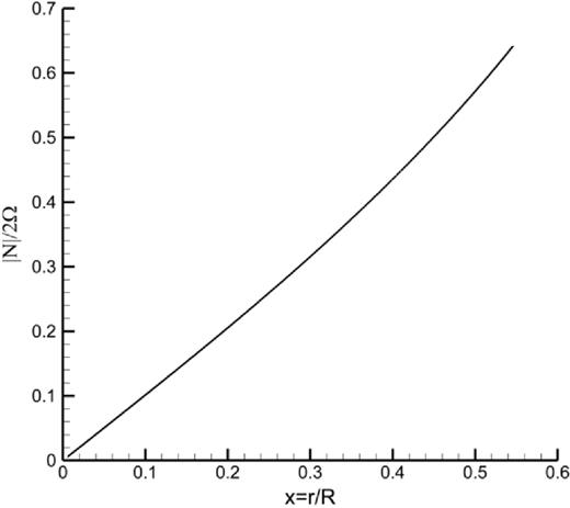
The non-dimensional Brant-Väisälä frequency, N/2Ω, in the modified spherical fluid core with |β| = 0.005 from eq. (9).

Open in new tab Download slide

The Galerkin procedure used to solve the dynamical equations is given in Seyed-Mahmoud & Rochester (2006). The mantle and the inner core are considered rigid, therefore, |${{\bf \hat{n}}}\cdot {{\bf u}}=0$| at the inner core boundary, ICB, where applicable, and the core mantle boundary, CMB. In the Earth's fluid core the additional stress due to deformation is given as |$\tilde{{\bf \tau }} = \lambda \, \zeta \tilde{\bf {1}}$|⁠, with |$\tilde{{\bf 1}}$| being the unit dyadic, while in the solid parts it takes the form

\begin{equation} \tilde{{\bf \tau }} = (\lambda {\nabla }\cdot {\bf u}) \tilde{{\bf 1}} +{\bf 2} \mu [{\nabla }{\bf u} +({\nabla }{\bf u})^{\rm T}] \end{equation}

(10)

with λ and μ being the Lamé parameters. For a rigid mantle (and inner core) the Lamé parameters become infinitely large and the displacement u becomes infinitely small in a manner that the resulting stress remains finite. To ensure that the normal component of the stress remains finite on the rigid side of the boundary we set

\begin{equation} | \hat{{\bf n}} \cdot \tilde{{\bf \tau }}|_{{\rm solid}\, {\rm side}} =\sum _{n=k}^{N_1} C_n^m \, P_n^m({\rm cos}\,\theta ) e^{i\,m\phi } \end{equation}

(11)

at the CMB and ICB, when applicable, where k = 3NL + |m|; 3NL refers to the number of equations, and the number of unknowns, resulting from the Galerkin formulation of eqs (1)–(3). After applying the Galerkin method to the continuity of the normal component of the stress tensor and using eq. (11) we get

\begin{equation} \int _S P_l^me^{-i\,m\phi }\Bigg\lbrace [\lambda \zeta ]_{{\rm fluid}\, {\rm side}} -\sum _{n=k}^{N_1} C_n^m \, P_n^m(\cos \,\theta )e^{i\,m\phi } \Bigg\rbrace {\rm d}S=0 \end{equation}

(12)

for l = k..N₁, and the integration is over the surface boundary. Adding these equations to the resulting Galerkin equations of eqs (1)–(3) and putting them into a matrix form we get

\begin{equation} \skew5\tilde{A}\bar{C}=0, \end{equation}

(13)

where |$\skew5\tilde{A}$| is the N1 × N1 coefficient matrix and |$\bar{C}$| is the array of size N₁ representing the constants. |$\skew5\tilde{A}$| may be written as

\begin{equation*} \left( \begin{array}{c@{\quad}c}\tilde{B} & \tilde{0} \\ \tilde{D} & \tilde{E} \\ \end{array} \right), \end{equation*}

where |$\tilde{D}$| and |$\tilde{E}$| are constructed from the first and second terms of eq. (12), and |$\tilde{B}$| is the resulting Galerkin matrix of eqs (1)–(3). Clearly, |$\tilde{E}$| is a unit matrix and its determinant is 1. Therefore, eq. (12) has no effects on the eigenvalues of |$\tilde{B}$|⁠, which are the frequencies of the inertial modes. In Seyed-Mahmoud & Moradi (2014), and initially in this article, we assumed that |${{\bf \hat{n}}}\cdot \tilde{{\bf \tau }}$| would vanish at the rigid boundaries. We would like to thank the reviewer of this article and Michael Rochester (private communications, 2014) for pointing out this error. The error, however, had not affected the results in either article.

Here we also review the boundary conditions which require the continuity in V₁ and |${{\bf \hat{n}}}\cdot {\nabla }V_1$|⁠, as |${{\bf \hat{n}}}\cdot {{\bf u}}=0$|⁠, across the fluid core boundaries to show that the gravitational flux may be written in terms of V₁ on the fluid side of the boundaries. Since the inner core and the mantle are assumed rigid, there are no mass movements in these regions and V₁ satisfies the Laplace's equation there

\begin{equation} V_1 (M)=\sum _{n=|m|}^{N} \frac{ a^m_n}{r^{n+1}}Y^m_n \end{equation}

(14)

in the mantle and

\begin{equation} V_1({\rm IC}) =\sum _{n=|m|}^N b^m_n r^{n} Y^m_n \end{equation}

(15)

in the inner core, when applicable.

Since the spherical harmonics are linearly independent, and noting that in the fluid core

\begin{equation} V_1={\sum }_{n} {\sum }_{l} \left(E^m_n\right)_l f_l (r) Y^m_n ({\rm cos} \theta ,\phi ) \end{equation}

(16)

for any m, the continuity of V₁ across the boundaries yields

\begin{equation} \sum _{l=0}^L \left(E^m_n\right)_l f_l(R_M)= \frac{a_n^m}{R_M^{n+1}} \end{equation}

(17)

at the CMB and

\begin{equation} \sum _{l=0}^L \left(E^m_n\right)_l f_l(R_{{\rm IC}})=b^m_n R_{{\rm IC}}^n \end{equation}

(18)

at the ICB, for n = 1..N, where R_M and R_IC are the radii of the CMB and the ICB, respectively. Eqs (17) and (18) are solved along with eqs (1)–(3) to satisfy the boundary conditions on V₁. Substituting for V₁ from eqs (14) and (15), the gravitational flux at the CMB and the ICB become

\begin{equation} {{\bf \hat{n}}} \cdot {\nabla }{V_1}(M)=- (n+1)\frac{a^m_n}{R_M^{n+2}} Y^m_n =-\frac{n+1}{R_M}V_1(M) \end{equation}

(19)

and

\begin{equation} {{\bf \hat{n}}} \cdot {\nabla }{V_1}({\rm IC})=n{b^m_n}{R_{{\rm IC}}^{n-1}} Y^m_n=\frac{n}{R_{{\rm IC}}} V_1({\rm IC}). \end{equation}

(20)

Therefore, since V₁ is continuous across the core boundaries, the continuity of the gravitational flux may be written in terms of the continuity of V₁ on the fluid side.

3 CORE MODELS

We adopt the fluid core of PREM as our core model and investigate the inertial modes of both a fluid sphere and spherical shell. As noted earlier, we take the reference state to be one of hydrostatic equilibrium in a frame rotating steadily at the rate Ωe₃. In this state, the figure of a rotating body is a spheroid and the radius of an equipotential surface is given as

\begin{equation} r=r_0 \left(1-\frac{2}{3}\varepsilon P_2({\rm cos} \theta )\right) \end{equation}

(21)

(Chandrasekhar & Roberts 1963) to first order in the ellipticity of the equipotential surfaces, where r₀ is the mean radius of the spherial equipotential surface, P₂ is the degree 2 Legendre polynomials and θ is the polar angle. Using PREM as the reference Earth model, ε has numerical values ranging from about 0.00247 at the ICB to about 0.00255 at the CMB while the stability parameter β has numerical values of approximately −0.028 near ICB and 0.010 near the CMB (Fig. 2). The effects of ellipticity on the frequencies of the core's inertial modes are small (Kudlick 1966), of the order of ellipticity (Seyed-Mahmoud & Moradi 2014). For example, the non-dimensional frequency, σ = ω/2Ω, of the (2, 1, 1) mode of the Poincaré model has numerical values of 0.5000 and 0.5013 for a spherical and a spheroidal geometries, respectively. Since in this work we intend to study the effects of non-zero β on the frequencies of the rotational modes of the core, we consider a first-order approximation in terms of the ellipticity, that is, ε = 0.

Figure 2.

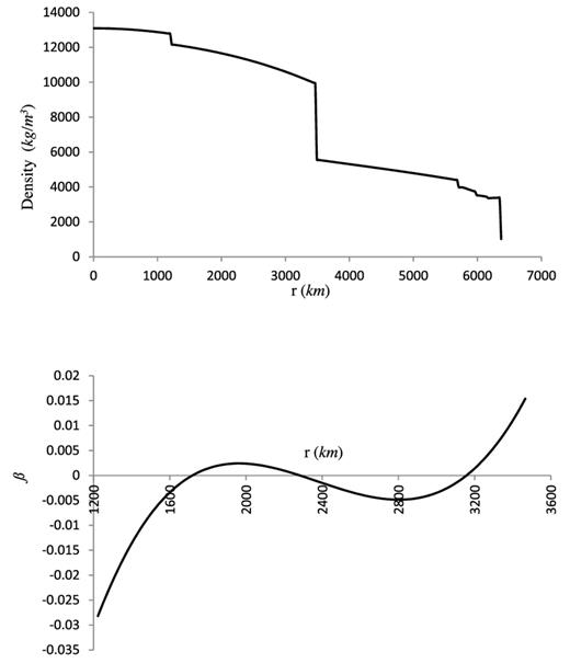
The density (top) and the stratification parameter profiles, bottom, for PREM Earth model.

Open in new tab Download slide

The objective of this work is to investigate the effects of non-neutral density stratification on the frequencies of the inertial-gravity modes of the core. As mentioned earlier, the Poincaré problem is ill-posed and analytical solutions do not exist in a thick rotating fluid shell geometry. The Poincaré operator, eq. (4), and the corresponding boundary conditions, vanishing of |$\hat{n}\cdot {{\bf u}}$| at the CMB and ICB, are embedded in the dynamical equations of a compressible core, eqs (1)–(3) and the corresponding boundary condition. Therefore, as explained by Seyed-Mahmoud & Rochester (2006), we expect that the frequencies of some of the modes of the fluid shell may not converge to three decimal points but fluctuate about their respective means. We, therefore, ignore the presence of the inner core for most of this work and make sure that the density ρ₀ and the compressional wave speed α profiles in the liquid core are extended to the centre of the Earth as smooth functions of the radius and that the mass of the core is conserved.

For a detailed description of density modification in the core for a specific β refer to Seyed-Mahmoud & Moradi (2014). We use the following profiles for the speed of the pressure waves, α, and the density, ρ₀, in the spherical fluid core models

\begin{equation} \alpha = 10.6776-8.7572 x^2\,\, {\rm km \,s}^{-1}, \end{equation}

(22)

\begin{equation} \rho _0=\sum _{n=1}^{12} d_n x^{n-1}, \end{equation}

(23)

where x = r/R, and R is the radius of the Earth. In Table 1, we show the coefficients of the density profile for the different core models we use in this paper.

Table 1.

Open in new tab

The coefficients of the density profile (kg m⁻³) for the spherical, compressible and stratified fluid core models.

d’s	β = −0.001	β = −0.002	β = −0.005	β = 0.001	β = 0.002	β = 0.005
d₁	1.2482 10⁴	1.2480 10⁴	1.2485 10⁴	1.2475 10⁴	1.2473 10⁴	1.2468 10⁴
d₂	0.0	0.0	0.0	0.0	0.0	0.0
d₃	− 7.7507 10³	− 7.7606 10³	− 7.7790 10³	− 7.7308 10³	− 7.7210 10³	− 7.6915 10³
d₄	4.2523 10^{− 2}	1.5008 10^{− 2}	5.0953 10^{− 2}	1.3254 10^{− 2}	6.0311 10^{− 2}	1.1308 10^{− 2}
d₅	− 2.5065 10³	− 2.5072 10³	− 2.5018 10³	− 2.5104 10³	− 2.5102 10³	− 2.5146 10³
d₆	1.4672 10¹	3.2642 10¹	1.6297 10¹	2.9605 10¹	1.7672 10¹	2.6303 10¹
d₇	− 9.6947 10²	− 1.0696 10³	− 9.7174 10²	− 1.0576 10²	− 9.9227 10²	− 1.0461 10³
d₈	5.1131 10²	8.7488 10²	5.4864 10²	8.1070 10²	5.7153 10²	7.4178 10²
d₉	− 1.7655 10³	− 2.5853 10³	− 1.8507 10³	− 2.4402 10³	− 1.9032 10³	− 2.2857 10³
d₁₀	2.6347 10³	3.7762 10³	2.7708 10³	3.5617 10³	2.8157 10³	3.3319 10³
d₁₁	− 2.7286 10³	− 3.6198 10³	− 2.8435 10³	− 3.4462 10³	− 2.8644 10³	− 3.2560 10³
d₁₂	1.1867 10³	1.4871 10³	1.2335 10³	1.4227 10³	1.1226 10³	1.3523 10³

d’s	β = −0.001	β = −0.002	β = −0.005	β = 0.001	β = 0.002	β = 0.005
d₁	1.2482 10⁴	1.2480 10⁴	1.2485 10⁴	1.2475 10⁴	1.2473 10⁴	1.2468 10⁴
d₂	0.0	0.0	0.0	0.0	0.0	0.0
d₃	− 7.7507 10³	− 7.7606 10³	− 7.7790 10³	− 7.7308 10³	− 7.7210 10³	− 7.6915 10³
d₄	4.2523 10^{− 2}	1.5008 10^{− 2}	5.0953 10^{− 2}	1.3254 10^{− 2}	6.0311 10^{− 2}	1.1308 10^{− 2}
d₅	− 2.5065 10³	− 2.5072 10³	− 2.5018 10³	− 2.5104 10³	− 2.5102 10³	− 2.5146 10³
d₆	1.4672 10¹	3.2642 10¹	1.6297 10¹	2.9605 10¹	1.7672 10¹	2.6303 10¹
d₇	− 9.6947 10²	− 1.0696 10³	− 9.7174 10²	− 1.0576 10²	− 9.9227 10²	− 1.0461 10³
d₈	5.1131 10²	8.7488 10²	5.4864 10²	8.1070 10²	5.7153 10²	7.4178 10²
d₉	− 1.7655 10³	− 2.5853 10³	− 1.8507 10³	− 2.4402 10³	− 1.9032 10³	− 2.2857 10³
d₁₀	2.6347 10³	3.7762 10³	2.7708 10³	3.5617 10³	2.8157 10³	3.3319 10³
d₁₁	− 2.7286 10³	− 3.6198 10³	− 2.8435 10³	− 3.4462 10³	− 2.8644 10³	− 3.2560 10³
d₁₂	1.1867 10³	1.4871 10³	1.2335 10³	1.4227 10³	1.1226 10³	1.3523 10³

Table 1.

Open in new tab

The coefficients of the density profile (kg m⁻³) for the spherical, compressible and stratified fluid core models.

d’s	β = −0.001	β = −0.002	β = −0.005	β = 0.001	β = 0.002	β = 0.005
d₁	1.2482 10⁴	1.2480 10⁴	1.2485 10⁴	1.2475 10⁴	1.2473 10⁴	1.2468 10⁴
d₂	0.0	0.0	0.0	0.0	0.0	0.0
d₃	− 7.7507 10³	− 7.7606 10³	− 7.7790 10³	− 7.7308 10³	− 7.7210 10³	− 7.6915 10³
d₄	4.2523 10^{− 2}	1.5008 10^{− 2}	5.0953 10^{− 2}	1.3254 10^{− 2}	6.0311 10^{− 2}	1.1308 10^{− 2}
d₅	− 2.5065 10³	− 2.5072 10³	− 2.5018 10³	− 2.5104 10³	− 2.5102 10³	− 2.5146 10³
d₆	1.4672 10¹	3.2642 10¹	1.6297 10¹	2.9605 10¹	1.7672 10¹	2.6303 10¹
d₇	− 9.6947 10²	− 1.0696 10³	− 9.7174 10²	− 1.0576 10²	− 9.9227 10²	− 1.0461 10³
d₈	5.1131 10²	8.7488 10²	5.4864 10²	8.1070 10²	5.7153 10²	7.4178 10²
d₉	− 1.7655 10³	− 2.5853 10³	− 1.8507 10³	− 2.4402 10³	− 1.9032 10³	− 2.2857 10³
d₁₀	2.6347 10³	3.7762 10³	2.7708 10³	3.5617 10³	2.8157 10³	3.3319 10³
d₁₁	− 2.7286 10³	− 3.6198 10³	− 2.8435 10³	− 3.4462 10³	− 2.8644 10³	− 3.2560 10³
d₁₂	1.1867 10³	1.4871 10³	1.2335 10³	1.4227 10³	1.1226 10³	1.3523 10³

d’s	β = −0.001	β = −0.002	β = −0.005	β = 0.001	β = 0.002	β = 0.005
d₁	1.2482 10⁴	1.2480 10⁴	1.2485 10⁴	1.2475 10⁴	1.2473 10⁴	1.2468 10⁴
d₂	0.0	0.0	0.0	0.0	0.0	0.0
d₃	− 7.7507 10³	− 7.7606 10³	− 7.7790 10³	− 7.7308 10³	− 7.7210 10³	− 7.6915 10³
d₄	4.2523 10^{− 2}	1.5008 10^{− 2}	5.0953 10^{− 2}	1.3254 10^{− 2}	6.0311 10^{− 2}	1.1308 10^{− 2}
d₅	− 2.5065 10³	− 2.5072 10³	− 2.5018 10³	− 2.5104 10³	− 2.5102 10³	− 2.5146 10³
d₆	1.4672 10¹	3.2642 10¹	1.6297 10¹	2.9605 10¹	1.7672 10¹	2.6303 10¹
d₇	− 9.6947 10²	− 1.0696 10³	− 9.7174 10²	− 1.0576 10²	− 9.9227 10²	− 1.0461 10³
d₈	5.1131 10²	8.7488 10²	5.4864 10²	8.1070 10²	5.7153 10²	7.4178 10²
d₉	− 1.7655 10³	− 2.5853 10³	− 1.8507 10³	− 2.4402 10³	− 1.9032 10³	− 2.2857 10³
d₁₀	2.6347 10³	3.7762 10³	2.7708 10³	3.5617 10³	2.8157 10³	3.3319 10³
d₁₁	− 2.7286 10³	− 3.6198 10³	− 2.8435 10³	− 3.4462 10³	− 2.8644 10³	− 3.2560 10³
d₁₂	1.1867 10³	1.4871 10³	1.2335 10³	1.4227 10³	1.1226 10³	1.3523 10³

For a spherical shell core model we adopt the fluid core of PREM and assume that the mantle and the inner core are rigid, as it is customary in computation of the inertial modes. Fig. 2 shows the density and the stratification parameter profiles for PREM. In the next section we use this model to compute the frequencies of the inertial-gravity modes of a shell as a more realistic model of the Earth's fluid core.

4 STABILITY PARAMETER AND THE INERTIAL MODES

As noted above, we use a Galerkin method to solve the governing eqs (1)–(3), including the boundary conditions. We first compute the frequencies of some of the low order, m = 0 and m = 1, and degree up to n = 6 inertial-gravity modes of six different spherical core models with β = −0.005, −0.003, −0.001, 0.001, 0.003 and 0.005. To ensure convergence we increase the number of terms appropriately (Seyed-Mahmoud & Rochester 2006).

In Tables 2 and 3, we show the frequencies of some of the modes we have been able to track down for the spherical core models with β < 0 and β > 0, respectively. We also show the frequencies for the Poincaré core model, for which analytical solutions exist (Greenspan 1969), Column 2 of Table 2. In columns next to the frequency columns we show the percentage differences for the respective frequencies compare to those for the Poincaré core model. The notation to identify a mode is that used by Greenspan (1969) (see also Seyed-Mahmoud & Rochester 2006). It is clear that for the set of modes we have computed, the frequencies of the (2, 1, 1), (3, 2, 1), (4, 3, 1), (5, 4, 1) and (6, 5, 1) modes are least affected by stratification. We note that these modes have the highest middle index number k for the respective n and m values. Except for the (6, 1, 1) mode, it seems that as k increases from 1 to n − 1, the effects of β decreases. From the data given in Tables 2 and 3 we infer that the frequency of a mode for a modified core model is smaller than the respective frequency of the Poincaré model if β > 0 and larger if β < 0 but not in a symmetric manner , that is, the percentage differences are not the same. The frequency of the (2, 1, 1) mode remains the same for all core models, as it should be, as predicted by theory (see e.g. Wahr 1981). In Figs 3 and 4 we have plotted the non-dimensional frequencies, σ, of the modes we have computed as a function of the stability parameter, β, for the wavenumber 1 and wavenumber 0 modes, respectively. These plots clearly show that the dependence of σ on β is linear for the range considered. Except for the (2, 1, 1), for which the slope is zero, the slopes of the frequency lines are negative if the frequencies are larger than 0 and positive otherwise. This means that as β changes from −0.005 to 0.005, the absolute value of a frequency decreases. These plots also reveal that it is possible that, for a specific value of β, two inertial-gravity modes have the same frequencies. For example, the lines of the frequencies of the (2, 1, 1) and (6, 3, 1) modes cross when β ≈ 0.002, and those of the (6, 1, 0) and (3, 1, 0) modes cross when β ≈ 0.0022. This crossing of the frequencies was also observed by Rieutord & Valdettaro (1997) who investigated the inertial modes of a homogeneous and incompressible fluid shell of small viscosity. They show that as viscosity tends to zero, the frequencies of two modes which resemble that of the (4, 1, 0) mode cross and approach two different values, and that the two modes have very different eigenfunctions.

Figure 3.

Non-dimensional frequency, σ, as a function of β for some of the wavenumber 1 modes of a spherical fluid core as β varies from −0.005 to 0.005. In the equation shown for each line, y represents the frequency and x the stability parameter.

Open in new tab Download slide

Figure 4.

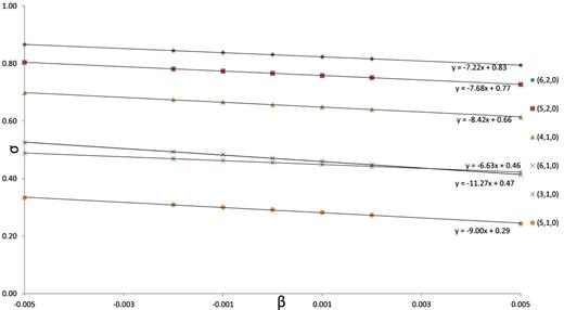
Non-dimensional frequency, σ, as a function of the stability parameter, β, for some of the wavenumber 0 modes of a spherical fluid core as β varies from −0.005 to 0.005. In the equation shown for each line, y represents the frequency and x the stability parameter.

Open in new tab Download slide

Table 2.

Open in new tab

Non-dimensional frequencies σ = ω/2Ω of some of the low-order inertial-gravity modes of a compressible and stratified spherical fluid core models with different stability parameter β. The column next to the right of a frequency column show the percentage difference between the respective modal frequencies of the specific core model and those of the Poincaré core model.

Mode	σ_pc	σ_−0.001	Per cent diff	σ_−0.002	Per cent diff	σ_−0.005	Per cent diff
(3, 1, 0)	0.447	0.463	3.6	0.469	4.9	0.488	9.2
(4, 1, 0)	0.655	0.666	1.7	0.674	2.9	0.698	6.6
(5, 1, 0)	0.285	0.300	5.3	0.309	8.4	0.333	17
(5, 2, 0)	0.765	0.774	1.2	0.781	2.1	0.804	5.1
(6, 1, 0)	0.469	0.483	3.0	0.493	5.1	0.525	12
(6, 2, 0)	0.830	0.838	1.0	0.845	1.8	0.866	4.3
(2, 1, 1)	0.500	0.500	0.0	0.500	0.0	0.500	0.0
(3, 2, 1)	0.755	0.754	0.1	0.759	0.5	0.776	2.8
(4, 1, 1)	− 0.410	− 0.434	2.6	− 0.447	9.0	− 0.483	18
(4, 2, 1)	0.306	0.314	5.9	0.318	3.9	0.329	7.5
(4, 3, 1)	0.854	0.854	0.0	0.859	0.6	0.874	2.3
(5, 1, 1)	− 0.592	− 0.609	2.9	− 0.621	4.9	− 0.655	11
(5, 3, 1)	0.523	0.532	1.7	0.541	3.4	0.569	8.8
(5, 4, 1)	0.903	0.904	0.1	0.909	0.7	0.923	2.2
(6, 1, 1)	− 0.702	− 0.716	2.0	− 0.726	3.4	− 0.757	7.8
(6, 2, 1)	− 0.269	− 0.290	7.8	− 0.303	13	− 0.340	26
(6, 3, 1)	0.220	0.231	5.0	0.237	7.7	0.255	16
(6, 4, 1)	0.653	0.660	1.1	0.669	2.5	0.694	6.3
(6, 5, 1)	0.931	0.933	0.2	0.937	0.6	0.950	2.0

Mode	σ_pc	σ_−0.001	Per cent diff	σ_−0.002	Per cent diff	σ_−0.005	Per cent diff
(3, 1, 0)	0.447	0.463	3.6	0.469	4.9	0.488	9.2
(4, 1, 0)	0.655	0.666	1.7	0.674	2.9	0.698	6.6
(5, 1, 0)	0.285	0.300	5.3	0.309	8.4	0.333	17
(5, 2, 0)	0.765	0.774	1.2	0.781	2.1	0.804	5.1
(6, 1, 0)	0.469	0.483	3.0	0.493	5.1	0.525	12
(6, 2, 0)	0.830	0.838	1.0	0.845	1.8	0.866	4.3
(2, 1, 1)	0.500	0.500	0.0	0.500	0.0	0.500	0.0
(3, 2, 1)	0.755	0.754	0.1	0.759	0.5	0.776	2.8
(4, 1, 1)	− 0.410	− 0.434	2.6	− 0.447	9.0	− 0.483	18
(4, 2, 1)	0.306	0.314	5.9	0.318	3.9	0.329	7.5
(4, 3, 1)	0.854	0.854	0.0	0.859	0.6	0.874	2.3
(5, 1, 1)	− 0.592	− 0.609	2.9	− 0.621	4.9	− 0.655	11
(5, 3, 1)	0.523	0.532	1.7	0.541	3.4	0.569	8.8
(5, 4, 1)	0.903	0.904	0.1	0.909	0.7	0.923	2.2
(6, 1, 1)	− 0.702	− 0.716	2.0	− 0.726	3.4	− 0.757	7.8
(6, 2, 1)	− 0.269	− 0.290	7.8	− 0.303	13	− 0.340	26
(6, 3, 1)	0.220	0.231	5.0	0.237	7.7	0.255	16
(6, 4, 1)	0.653	0.660	1.1	0.669	2.5	0.694	6.3
(6, 5, 1)	0.931	0.933	0.2	0.937	0.6	0.950	2.0

Table 2.

Open in new tab

Non-dimensional frequencies σ = ω/2Ω of some of the low-order inertial-gravity modes of a compressible and stratified spherical fluid core models with different stability parameter β. The column next to the right of a frequency column show the percentage difference between the respective modal frequencies of the specific core model and those of the Poincaré core model.

Mode	σ_pc	σ_−0.001	Per cent diff	σ_−0.002	Per cent diff	σ_−0.005	Per cent diff
(3, 1, 0)	0.447	0.463	3.6	0.469	4.9	0.488	9.2
(4, 1, 0)	0.655	0.666	1.7	0.674	2.9	0.698	6.6
(5, 1, 0)	0.285	0.300	5.3	0.309	8.4	0.333	17
(5, 2, 0)	0.765	0.774	1.2	0.781	2.1	0.804	5.1
(6, 1, 0)	0.469	0.483	3.0	0.493	5.1	0.525	12
(6, 2, 0)	0.830	0.838	1.0	0.845	1.8	0.866	4.3
(2, 1, 1)	0.500	0.500	0.0	0.500	0.0	0.500	0.0
(3, 2, 1)	0.755	0.754	0.1	0.759	0.5	0.776	2.8
(4, 1, 1)	− 0.410	− 0.434	2.6	− 0.447	9.0	− 0.483	18
(4, 2, 1)	0.306	0.314	5.9	0.318	3.9	0.329	7.5
(4, 3, 1)	0.854	0.854	0.0	0.859	0.6	0.874	2.3
(5, 1, 1)	− 0.592	− 0.609	2.9	− 0.621	4.9	− 0.655	11
(5, 3, 1)	0.523	0.532	1.7	0.541	3.4	0.569	8.8
(5, 4, 1)	0.903	0.904	0.1	0.909	0.7	0.923	2.2
(6, 1, 1)	− 0.702	− 0.716	2.0	− 0.726	3.4	− 0.757	7.8
(6, 2, 1)	− 0.269	− 0.290	7.8	− 0.303	13	− 0.340	26
(6, 3, 1)	0.220	0.231	5.0	0.237	7.7	0.255	16
(6, 4, 1)	0.653	0.660	1.1	0.669	2.5	0.694	6.3
(6, 5, 1)	0.931	0.933	0.2	0.937	0.6	0.950	2.0

Mode	σ_pc	σ_−0.001	Per cent diff	σ_−0.002	Per cent diff	σ_−0.005	Per cent diff
(3, 1, 0)	0.447	0.463	3.6	0.469	4.9	0.488	9.2
(4, 1, 0)	0.655	0.666	1.7	0.674	2.9	0.698	6.6
(5, 1, 0)	0.285	0.300	5.3	0.309	8.4	0.333	17
(5, 2, 0)	0.765	0.774	1.2	0.781	2.1	0.804	5.1
(6, 1, 0)	0.469	0.483	3.0	0.493	5.1	0.525	12
(6, 2, 0)	0.830	0.838	1.0	0.845	1.8	0.866	4.3
(2, 1, 1)	0.500	0.500	0.0	0.500	0.0	0.500	0.0
(3, 2, 1)	0.755	0.754	0.1	0.759	0.5	0.776	2.8
(4, 1, 1)	− 0.410	− 0.434	2.6	− 0.447	9.0	− 0.483	18
(4, 2, 1)	0.306	0.314	5.9	0.318	3.9	0.329	7.5
(4, 3, 1)	0.854	0.854	0.0	0.859	0.6	0.874	2.3
(5, 1, 1)	− 0.592	− 0.609	2.9	− 0.621	4.9	− 0.655	11
(5, 3, 1)	0.523	0.532	1.7	0.541	3.4	0.569	8.8
(5, 4, 1)	0.903	0.904	0.1	0.909	0.7	0.923	2.2
(6, 1, 1)	− 0.702	− 0.716	2.0	− 0.726	3.4	− 0.757	7.8
(6, 2, 1)	− 0.269	− 0.290	7.8	− 0.303	13	− 0.340	26
(6, 3, 1)	0.220	0.231	5.0	0.237	7.7	0.255	16
(6, 4, 1)	0.653	0.660	1.1	0.669	2.5	0.694	6.3
(6, 5, 1)	0.931	0.933	0.2	0.937	0.6	0.950	2.0

Table 3.

Open in new tab

Non-dimensional frequencies, σ = ω/2Ω of some of the low-order inertial-gravity modes of compressible and stratified spherical fluid core models with different stability parameter β. The column next to the right of a frequency column show the absolute percentage differences between the respective frequencies of the specific core model and those of the Poincaré core model (Column 2 of Table 2).

Mode	σ_0.001	Per cent diff	σ_0.002	Per cent diff	σ_0.005	Per cent diff
(3, 1, 0)	0.449	0.4	0.442	1.1	0.422	5.6
(4, 1, 0)	0.649	0.9	0.640	2.3	0.614	6.3
(5, 1, 0)	0.282	1.1	0.273	4.2	0.243	14.7
(5, 2, 0)	0.758	0.9	0.751	1.8	0.727	5.0
(6, 1, 0)	0.460	1.9	0.449	4.3	0.412	12.2
(6, 2, 0)	0.823	0.8	0.816	1.7	0.794	4.3
(2, 1, 1)	0.500	0.0	0.500	0.0	0.500	0.0
(3, 2, 1)	0.743	1.6	0.737	2.4	0.720	4.6
(4, 1, 1)	− 0.408	0.5	− 0.394	3.9	− 0.350	14.6
(4, 2, 1)	0.306	0.0	0.302	1.3	0.290	5.2
(4, 3, 1)	0.844	1.2	0.839	1.8	0.824	3.5
(5, 1, 1)	− 0.586	1.0	− 0.574	3.0	− 0.536	9.5
(5, 3, 1)	0.512	2.1	0.502	4.0	0.471	9.9
(5, 4, 1)	0.895	0.9	0.890	1.4	0.876	3.0
(6, 1, 1)	− 0.703	0.1	− 0.685	2.4	− 0.652	7.1
(6, 2, 1)	− 0.261	3.0	− 0.246	8.6	− 0.194	27.9
(6, 3, 1)	0.217	1.4	0.210	4.5	0.190	13.6
(6, 4, 1)	0.643	1.5	0.634	2.9	0.607	7.0
(6, 5, 1)	0.924	0.8	0.919	1.3	0.906	2.7

Mode	σ_0.001	Per cent diff	σ_0.002	Per cent diff	σ_0.005	Per cent diff
(3, 1, 0)	0.449	0.4	0.442	1.1	0.422	5.6
(4, 1, 0)	0.649	0.9	0.640	2.3	0.614	6.3
(5, 1, 0)	0.282	1.1	0.273	4.2	0.243	14.7
(5, 2, 0)	0.758	0.9	0.751	1.8	0.727	5.0
(6, 1, 0)	0.460	1.9	0.449	4.3	0.412	12.2
(6, 2, 0)	0.823	0.8	0.816	1.7	0.794	4.3
(2, 1, 1)	0.500	0.0	0.500	0.0	0.500	0.0
(3, 2, 1)	0.743	1.6	0.737	2.4	0.720	4.6
(4, 1, 1)	− 0.408	0.5	− 0.394	3.9	− 0.350	14.6
(4, 2, 1)	0.306	0.0	0.302	1.3	0.290	5.2
(4, 3, 1)	0.844	1.2	0.839	1.8	0.824	3.5
(5, 1, 1)	− 0.586	1.0	− 0.574	3.0	− 0.536	9.5
(5, 3, 1)	0.512	2.1	0.502	4.0	0.471	9.9
(5, 4, 1)	0.895	0.9	0.890	1.4	0.876	3.0
(6, 1, 1)	− 0.703	0.1	− 0.685	2.4	− 0.652	7.1
(6, 2, 1)	− 0.261	3.0	− 0.246	8.6	− 0.194	27.9
(6, 3, 1)	0.217	1.4	0.210	4.5	0.190	13.6
(6, 4, 1)	0.643	1.5	0.634	2.9	0.607	7.0
(6, 5, 1)	0.924	0.8	0.919	1.3	0.906	2.7

Table 3.

Open in new tab

Non-dimensional frequencies, σ = ω/2Ω of some of the low-order inertial-gravity modes of compressible and stratified spherical fluid core models with different stability parameter β. The column next to the right of a frequency column show the absolute percentage differences between the respective frequencies of the specific core model and those of the Poincaré core model (Column 2 of Table 2).

Mode	σ_0.001	Per cent diff	σ_0.002	Per cent diff	σ_0.005	Per cent diff
(3, 1, 0)	0.449	0.4	0.442	1.1	0.422	5.6
(4, 1, 0)	0.649	0.9	0.640	2.3	0.614	6.3
(5, 1, 0)	0.282	1.1	0.273	4.2	0.243	14.7
(5, 2, 0)	0.758	0.9	0.751	1.8	0.727	5.0
(6, 1, 0)	0.460	1.9	0.449	4.3	0.412	12.2
(6, 2, 0)	0.823	0.8	0.816	1.7	0.794	4.3
(2, 1, 1)	0.500	0.0	0.500	0.0	0.500	0.0
(3, 2, 1)	0.743	1.6	0.737	2.4	0.720	4.6
(4, 1, 1)	− 0.408	0.5	− 0.394	3.9	− 0.350	14.6
(4, 2, 1)	0.306	0.0	0.302	1.3	0.290	5.2
(4, 3, 1)	0.844	1.2	0.839	1.8	0.824	3.5
(5, 1, 1)	− 0.586	1.0	− 0.574	3.0	− 0.536	9.5
(5, 3, 1)	0.512	2.1	0.502	4.0	0.471	9.9
(5, 4, 1)	0.895	0.9	0.890	1.4	0.876	3.0
(6, 1, 1)	− 0.703	0.1	− 0.685	2.4	− 0.652	7.1
(6, 2, 1)	− 0.261	3.0	− 0.246	8.6	− 0.194	27.9
(6, 3, 1)	0.217	1.4	0.210	4.5	0.190	13.6
(6, 4, 1)	0.643	1.5	0.634	2.9	0.607	7.0
(6, 5, 1)	0.924	0.8	0.919	1.3	0.906	2.7

Mode	σ_0.001	Per cent diff	σ_0.002	Per cent diff	σ_0.005	Per cent diff
(3, 1, 0)	0.449	0.4	0.442	1.1	0.422	5.6
(4, 1, 0)	0.649	0.9	0.640	2.3	0.614	6.3
(5, 1, 0)	0.282	1.1	0.273	4.2	0.243	14.7
(5, 2, 0)	0.758	0.9	0.751	1.8	0.727	5.0
(6, 1, 0)	0.460	1.9	0.449	4.3	0.412	12.2
(6, 2, 0)	0.823	0.8	0.816	1.7	0.794	4.3
(2, 1, 1)	0.500	0.0	0.500	0.0	0.500	0.0
(3, 2, 1)	0.743	1.6	0.737	2.4	0.720	4.6
(4, 1, 1)	− 0.408	0.5	− 0.394	3.9	− 0.350	14.6
(4, 2, 1)	0.306	0.0	0.302	1.3	0.290	5.2
(4, 3, 1)	0.844	1.2	0.839	1.8	0.824	3.5
(5, 1, 1)	− 0.586	1.0	− 0.574	3.0	− 0.536	9.5
(5, 3, 1)	0.512	2.1	0.502	4.0	0.471	9.9
(5, 4, 1)	0.895	0.9	0.890	1.4	0.876	3.0
(6, 1, 1)	− 0.703	0.1	− 0.685	2.4	− 0.652	7.1
(6, 2, 1)	− 0.261	3.0	− 0.246	8.6	− 0.194	27.9
(6, 3, 1)	0.217	1.4	0.210	4.5	0.190	13.6
(6, 4, 1)	0.643	1.5	0.634	2.9	0.607	7.0
(6, 5, 1)	0.924	0.8	0.919	1.3	0.906	2.7

In Fig. 5, we show the displacement eigenfunctions, as well as the contour plots of the dilatation, ζ, for the (2, 1, 1) mode, (4, 1, 1) and (6, 5, 1) modes for Earth models with β = 0.0 and β = −0.005. The choice of these modes is based on the effects of β on the frequencies of these modes, which is zero for the (2, 1, 1) mode, small on the (6, 5, 1) mode and large on the (4, 1, 1) mode. In Fig. 6 we show the plots for the same modes as in Fig. 5 but for a core model with β = 0.005. The plots for the (2, 1, 1) show that the flow is practically divergence free. Note the numerical solutions are based on the truncated trial functions. We have used a minimum of 27 terms, N = 3 and L = 3, to compute the frequency and the eigenfunctions for the (2, 1, 1) mode. We suspect that the small non-zero divergence appearing in the plots of this mode is due to computational errors. In Table 2, the frequencies are reported accurate to three decimal points. The frequency of the (2, 1, 1) mode converged to 0.49997. For a divergence free flow, eq. (2) reduces to the Poincaré equation, therefore, we expect that the core models are irrelevant for this mode and that its frequency remains at 0.500 regardless of the core model. In Fig. 7, we show the contour plots for the flow pressure for the respective modes in Fig. 5. The pressure contours for the respective modes are similar in both models. For the (6, 5, 1) mode, for which the effects of stratification is relatively small, the modal cells for the displacement are formed predominantly perpendicular to the rotation axis, while for the (4, 1, 1) mode these cells are formed predominantly parallel to the rotation axis. Using a cylindrical coordinate system (ρ, ϕ, z), the z component of eq. (7) becomes

\begin{equation} \sigma ^2 w=\frac{\partial \Psi }{\partial z}+\beta g_0\,\, {\rm cos}(\theta ) \zeta , \end{equation}

(24)

where w is the z component of u, |$\sigma =\frac{\omega }{2 \Omega }$|⁠, |$\Psi = \frac{\chi -V_1}{4 R^2 \Omega ^2}$|⁠, g₀ is non-dimensionalized by dividing it by 4RΩ², and θ = sin ⁻¹(ρ/r) is the colatitude. The radial component of this equation takes the form

\begin{equation} \sigma \left[(\sigma ^2-1)u_{\rho }-\frac{\partial \Psi }{\partial \rho }-\beta \sin \theta g_0 \zeta \right]=\frac{\Psi }{\rho }, \end{equation}

(25)

where ρ has been non-dimensionalized by dividing it by R. In eq. (24), the frequency σ has stronger dependence on β than it does in eq. (25). It seems, then, that the stronger the parallel components of the displacement vectors to the rotation axis, the stronger the effects of the stratification is on the frequency of the mode. To support this statement we have plotted in Fig. 8 the displacement vectors for six more modes of a sphere which frequencies are reported in Table 2.

Figure 5.

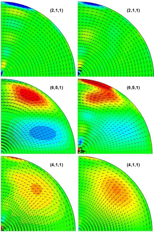
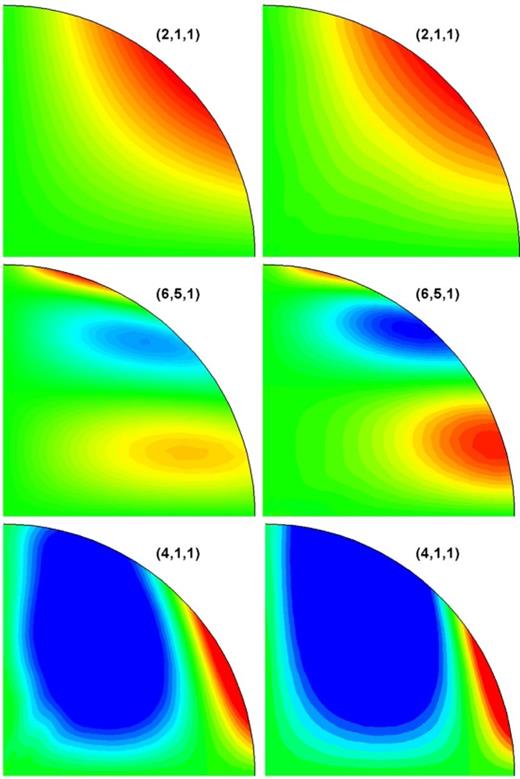
The displacement eigenfunctions and the contour plots of the dilatation, ζ = ∇ · u, for some of the modes of a neutrally stratified, β = 0, core model (left) and their counterparts for a core model with β = −0.005 (right).

Open in new tab Download slide

Figure 6.

The displacement eigenfunctions and the contour plots of the dilatation for the modes in Fig. 5 for a core model with β = 0.005.

Open in new tab Download slide

Figure 7.

Contour plots of the non-dimensional pressure, χ, for the modes in Fig. 5.

Open in new tab Download slide

Figure 8.

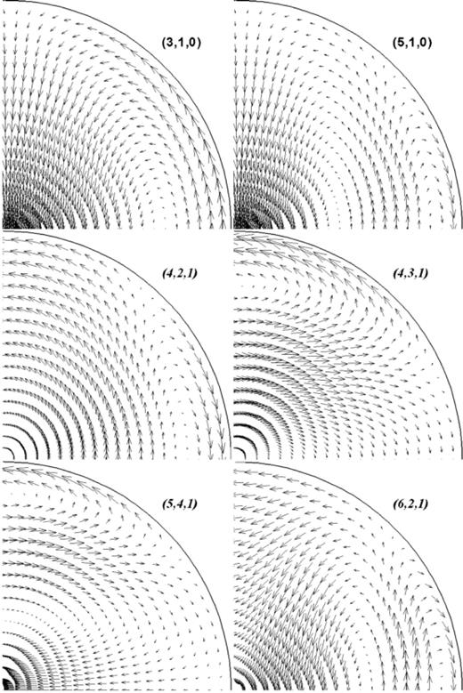
The displacement eigenfunctions for some of the inertial modes of a sphere. The frequencies of the modes with displacement cells parallel to the rotation axis, vertical, are affected by stratification more than those with the same perpendicular to that axis.

Open in new tab Download slide

For a fluid shell models we use the density and the stratification parameter profiles of PREM shown in Fig. 2 and assume that the boundaries are rigid. In Table 4, we show the frequencies of some of the low-order modes of this model for (1) a neutrally stratified core, Column 2, after Seyed-Mahmoud et al. (2007) and (2) the corresponding values for PREM fluid core model, Column 3. Some of the corresponding displacement eigenfunctions are given in Fig. 9. For this model some the frequencies converged to two decimal points and some to three. Even so, the eigenfunctions in Fig. 9 show that these are indeed the frequencies of the inertial modes. We emphasize that compressibility had been accounted for in computing the modal frequencies of a neutrally stratified core model (Seyed-Mahmoud et al.2007).

Figure 9.

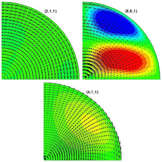
The displacement eigenfunctions for some the inertial modes of PREM.

Open in new tab Download slide

Table 4.

Open in new tab

Non-dimensional frequencies σ = ω/2Ω of some of the low-order inertial modes of a compressible and stratified fluid shell. In Columns 2 and 3 we show these frequencies for a neutrally stratified core, taken from Seyed-Mahmoud et al. (2007), and those for PREM core model.

Mode	σ_neut	σ_PREM	Per cent diff
(2, 1, 1)	0.500	0.500	0
(4, 1, 0)	0.664	0.673	1.3
(4, 2, 1)	0.304	0.313	3.0
(4, 3, 1)	0.852	0.86	0.9
(5, 4, 1)	0.932	0.940	1.1
(6, 2, 0)	0.833	0.84	0.8
(6, 4, 1)	0.657	0.670	1.5

Mode	σ_neut	σ_PREM	Per cent diff
(2, 1, 1)	0.500	0.500	0
(4, 1, 0)	0.664	0.673	1.3
(4, 2, 1)	0.304	0.313	3.0
(4, 3, 1)	0.852	0.86	0.9
(5, 4, 1)	0.932	0.940	1.1
(6, 2, 0)	0.833	0.84	0.8
(6, 4, 1)	0.657	0.670	1.5

Table 4.

Open in new tab

Non-dimensional frequencies σ = ω/2Ω of some of the low-order inertial modes of a compressible and stratified fluid shell. In Columns 2 and 3 we show these frequencies for a neutrally stratified core, taken from Seyed-Mahmoud et al. (2007), and those for PREM core model.

Mode	σ_neut	σ_PREM	Per cent diff
(2, 1, 1)	0.500	0.500	0
(4, 1, 0)	0.664	0.673	1.3
(4, 2, 1)	0.304	0.313	3.0
(4, 3, 1)	0.852	0.86	0.9
(5, 4, 1)	0.932	0.940	1.1
(6, 2, 0)	0.833	0.84	0.8
(6, 4, 1)	0.657	0.670	1.5

Mode	σ_neut	σ_PREM	Per cent diff
(2, 1, 1)	0.500	0.500	0
(4, 1, 0)	0.664	0.673	1.3
(4, 2, 1)	0.304	0.313	3.0
(4, 3, 1)	0.852	0.86	0.9
(5, 4, 1)	0.932	0.940	1.1
(6, 2, 0)	0.833	0.84	0.8
(6, 4, 1)	0.657	0.670	1.5

5 CONCLUSION

In this work, we show that the effects of density stratification with different stratification parameter β on the frequencies of the rotational modes of the Earth's core may be very significant. For example, the non-dimensional frequency of the (6, 2, 1) inertial mode of a sphere is adjusted from −0.269 for the Poincaré core model to −0.340 for a core mode with the stability parameter of −0.005, a change of about 26 per cent. We also show that for small stratification parameter, |β| ≤ 0.005, the frequency of an inertial-gravity mode is a nearly linear function of β but the slope of the line is different for different modes. From the displacement patterns of the modes in Figs. 5 and 8, and eqs (24) and (25) we deduce that the effect of the stratification is likely related to the spatial structure, in terms of displacement eigenfunctions, of the modes. We have also shown that if, during the excitation of a mode, the flow is solenoidal, that is ∇ · u = 0, then the frequency of the mode is not affected by density stratification. This is also clear from eq. (7), since taking the divergence of this equation and using the reduced potential ξ = χ − V₁ we get

\begin{equation*} {{\nabla }}\cdot ( {\bf \tilde{\Gamma }}_{\bf p}{\cdot {{{\nabla }}\xi }})=0 \end{equation*}

which is the Poincaré equation. Therefore, the material properties are irrelevant if the flow is solenoidal.

This work was supported by the Natural Sciences and Engineering Research Council of Canada (NSERC) Discovery Grant program and the University of Lethbridge Research Fund (ULRF). We sincerely thank two anonymous reviewers who examined this article carefully and made comments that helped correct some mistakes and clarify some points.

REFERENCES

Aldridge

K.D.

An experimental study of axisymmetric inertial oscillations of a rotating liquid sphere

PhD thesis

1967

Massachusetts Institute of Technology

Month:	Total Views:
February 2017	3
April 2017	1
July 2017	1
August 2017	2
October 2017	1
November 2017	1
March 2018	2
April 2018	2
May 2018	1
August 2018	12
September 2018	3
October 2018	4
November 2018	12
December 2018	4
January 2019	2
February 2019	7
March 2019	12
April 2019	7
May 2019	12
June 2019	3
July 2019	11
August 2019	8
September 2019	5
October 2019	8
November 2019	18
December 2019	7
January 2020	5
February 2020	5
March 2020	4
April 2020	7
May 2020	5
June 2020	4
July 2020	9
August 2020	17
September 2020	17
October 2020	8
November 2020	8
December 2020	4
January 2021	6
February 2021	3

Article Contents

Effects of density stratification on the frequencies of the inertial-gravity modes of the Earth's fluid core Free

Abstract

1 INTRODUCTION

2 GOVERNING EQUATIONS

3 CORE MODELS

4 STABILITY PARAMETER AND THE INERTIAL MODES

5 CONCLUSION

REFERENCES

Citations

Views

Altmetric

Email alerts

Astrophysics Data System

Citing articles via

Latest

Most Read

Most Cited

This Feature Is Available To Subscribers Only

Effects of density stratification on the frequencies of the inertial-gravity modes of the Earth's fluid core