


Abstract
We have investigated the seismic anisotropy beneath the Central Andean southern Puna plateau by applying shear wave splitting analysis and shear wave splitting tomography to local S waves and teleseismic SKS, SKKS and PKS phases. Overall, a very complex pattern of fast directions throughout the southern Puna plateau region and a circular pattern of fast directions around the region of the giant Cerro Galan ignimbrite complex are observed. In general, teleseismic lag times are much greater than those for local events which are interpreted to reflect a significant amount of sub and inner slab anisotropy. The complex pattern observed from shear wave splitting analysis alone is the result of a complex 3-D anisotropic structure under the southern Puna plateau. Our application of shear wave splitting tomography provides a 3-D model of anisotropy in the southern Puna plateau that shows different patterns depending on the driving mechanism of upper-mantle flow and seismic anisotropy. The trench parallel a-axes in the continental lithosphere above the slab east of 68W may be related to deformation of the overriding continental lithosphere since it is under compressive stresses which are orthogonal to the trench. The more complex pattern below the Cerro Galan ignimbrite complex and above the slab is interpreted to reflect delamination of continental lithosphere and upwelling of hot asthenosphere. The a-axes beneath the Cerro Galan, Cerro Blanco and Carachi Pampa volcanic centres at 100 km depth show some weak evidence for vertically orientated fast directions, which could be due to vertical asthenospheric flow around a delaminated block. Additionally, our splitting tomographic model shows that there is a significant amount of seismic anisotropy beneath the slab. The subslab mantle west of 68W shows roughly trench parallel horizontal a-axes that are probably driven by slab roll back and the relatively small coupling between the Nazca slab and the underlying mantle. In contrast, the subslab region (i.e. depths greater than 200 km) east of 68W shows a circular pattern of a-axes centred on a region with small strength of anisotropy (Cerro Galan and its eastern edge) which suggest the dominant mechanism is a combination of slab roll back and flow driven by an overlying abnormally heated slab or possibly a slab gap. There seems to be some evidence for vertical flow below the slab at depths of 200–400 km driven by the abnormally heated slab or slab gap. This cannot be resolved by the tomographic inversion due to the lack of ray crossings in the subslab mantle.
1 INTRODUCTION
The southern Puna plateau of the central Andes offers an excellent natural laboratory to study the distribution of seismic anisotropy in a region with a spatially changing subduction angle (e.g. Cahill & Isacks 1992; Mulcahy et al.2014) and where crustal and mantle lithospheric delamination has been argued to have occurred (e.g. Kay et al.1994; Calixto et al.2013; Liang et al.2014) to explain geologic and geophysical observations including the existence of mafic lavas and giant ignimbrites, a gap of intermediate-depth seismicity, and high topography with large deficit in crustal shortening. Regionally, the southern Puna constitutes the southernmost part of the central Andean Altiplano-Puna plateau (Figs 1 and 2; see review by Allmendinger et al.1997). The region is generally characterized by a thin 60–80-km-thick lithosphere with a crustal thickness varying from 40 to 70 km (Heit et al.2014). Crustal thickening related to crustal shortening has been argued to account for 70–80 per cent of the crustal thickness observed (Allmendinger et al.1997) with the rest being attributed to magmatic addition, crustal flow and thermal uplift (Isacks 1988; Whitman et al.1996). The thermal uplift has been argued to be due to mechanical thinning of the lithosphere by delamination (e.g. Kay & Kay 1993; Kay et al.1994; Bianchi et al.2013; Calixto et al.2013; Liang et al.2014) with decompression melting after delamination in an expanding mantle wedge over a steepening subduction zone being the source of the thermal uplift (Kay & Coira 2009; Risse et al.2013). The thermal effects of crustal and lithospheric delamination have been associated with the distinctive southern Puna mafic volcanism and giant ignimbrite eruptions, a gap in intermediate depth seismicity (e.g. Mulcahy et al.2014) and a late Miocene change (Risse et al.2008) from an uniformly compressive to more chaotic stress regime (e.g. Marrett et al.1994). A high velocity body above the slab under the Cerro Galan ignimbrite region has been interpreted as the most recent delaminated block (Calixto et al.2013).
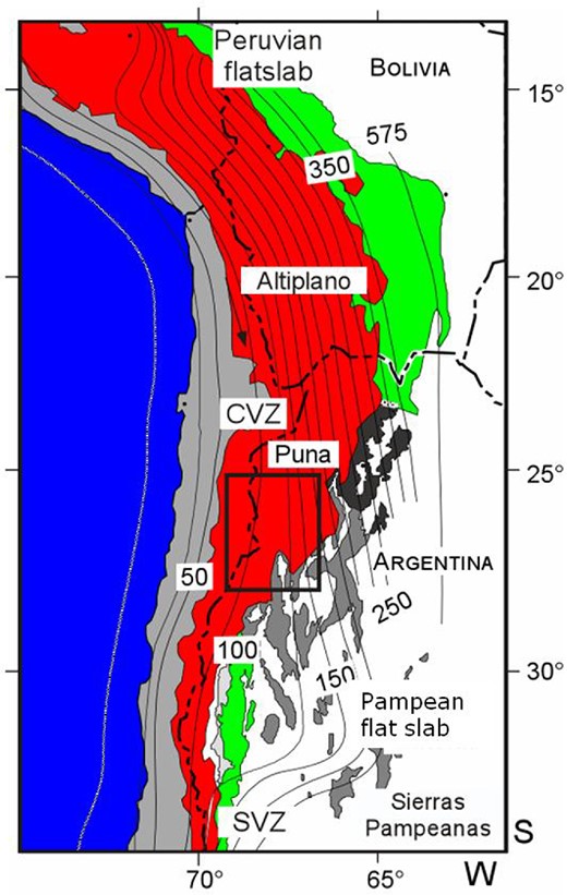
Andean Orogeny and region of study—Southern Puna Plateau, shown in the black rectangle. From west to east: Pacific ocean (blue), region below 3 km elevation including the coastal area (light grey), Altiplano-Puna plateau (red), thin-skinned thrust belts (green), thick-skinned deformation regions in Santa Barbara (black) and Sierras Pampeanas (grey). The central and southern volcanic zones (CVZ and SVZ) are also shown. The thin black curves represent the slab depth contours in km (Cahill & Isacks 1992) and show the northward transition from shallow subduction to normal subduction.
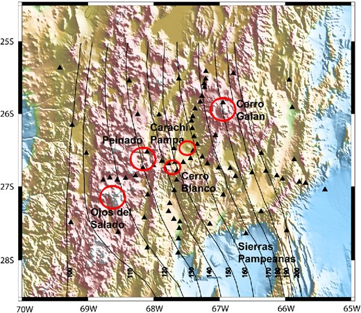
Seismic station distribution (black triangles) along the Southern Puna Plateau. Cerro Galan, Ojos del Salado, Cerro Blanco, Carachi Pampa and Peinado volcanic centres are shown in red circles. Sierras Pampeanas flat subduction region is located southeast of the region of study. The slab contours from 100 to 200 km depth in 10 km intervals are also shown (Mulcahy et al.2014)
In order to understand the geodynamics of a subduction zone, with the added complexity of delamination, it is important to investigate the seismic anisotropy related to mantle flow around the subducting slab. This seismic anisotropy is produced by strain-induced lattice preferred orientation (LPO) of minerals in the upper mantle (Nicolas & Christensen 1987; Ribe & Yu 1991; Ribe 1992; Kaminski & Ribe 2002), which causes shear waves to split into fast and slow polarized waves. Seismic anisotropy in the asthenosphere is likely due to flow controlled by the subducting plate dynamics (Long & Silver 2008), and possibly by spatial variation of mantle density (e.g. Silver & Holt 2002). In the case of the Puna plateau, slab geometry (Mulcahy et al.2014), partially heated slab or possibly a slab gap (Calixto et al.2013) and delamination (Kay & Coira 2009; Calixto et al.2013) could play an additional role in generating the spatial contrast in density and consequently, cause localized flow and complex patterns of seismic anisotropy. Here, we use shear wave splitting analysis and shear wave splitting tomography to estimate the seismic anisotropy structure of the region and to investigate the effect of delamination on asthenospheric and lithospheric mantle flow. The seismic data used in the study were recorded on 43 U.S. and 30 German broad-band three component seismic stations in an array, which was deployed for approximately two years in the southern Puna project (Fig. 2; see Heit et al.2014; Mulcahy et al.2014).
2 SHEAR WAVE SPLITTING ANALYSIS
2.1 Methodology
This study uses both teleseismic SKS, SKKS and PKS and local shear waves to measure shear wave splitting, which occurs when a shear wave travels through an anisotropic medium, and investigate the seismic anisotropy in the southern Puna plateau. In general, mantle seismic anisotropy occurs when aggregates of anisotropic mantle minerals, particularly olivine and orthopyroxene, align in a coherent direction; also know as LPO. Previous studies have found that in the case of olivine this direction tends to be parallel to the direction of maximum finite strain (Ribe 1989). More recent studies have found that the relationship between LPO and maximum finite strain could be more complex involving other factors such as: strain rate (Kaminski & Ribe 2002), strain history, shear direction and dynamic recrystallization (Karato 1987), water and stress (Jung et al.2006), pressure (Mainprice et al.2005; Couvy et al.2004) and melt (Holtzman et al.2003; Kaminski 2006). Karato et al.2008, summarizes most of these factors. In summary, olivine a-axes align close to the direction of mantle flow in regions where flow patterns change slowly in space; however, the relationship of LPO to strain is more complex where the mantle flow is more complex. This means that the olivine a-axes will align close to the direction of flow only if the time it takes the LPO to develop is smaller than time over which the geometry of strain changes along the flow-lines (Kaminski & Ribe 2002).
If the LPO can be related with the direction of flow, or deformation, then shear wave splitting can be used to study the flow in the upper mantle. Shear wave splitting is then studied by measuring two parameters: the polarization of the fast shear wave component (φ) and the lag time between fast and slow split shear waves (dt). Here, both splitting parameters are estimated following Silver & Chan (1991) by minimizing the second eigenvalue in the covariance matrix formed by the horizontal components. In the case of teleseismic shear waves the splitting parameters were obtained by grid searching around the best parameters that minimize the energy in the tangential component. Quality control was performed by visually inspecting the radial versus tangential particle motion plot for all of the events after correcting for splitting. A linear particle motion indicates that the splitting has been successfully removed and estimated parameters are most likely reliable. In contrast, residual elliptical or more complex particle motions indicate the estimated parameters are unreliable, most commonly due to a low signal-to-noise ratio.
2.2 Data and observations
The southern Puna seismic array (Fig. 2) consists of 73 broad-band and short period stations that were deployed for a period of 2 yr starting in 2007. Shear wave splitting analysis was applied to both local and teleseismic events. The local events provide information on anisotropy between the slab and the surface whereas the teleseismic events elucidate anisotropy between the core–mantle boundary and the surface. Incidence angles for local events can vary between 0 and 90° whereas teleseismic incidence angles are typically less than 10°. In this study, we used local events with depths greater than 100 km and incidence angles less than 35° to avoid free surface effects, shallow interface phase shifts and phase conversions. Since local events have a variety of polarization directions and angles of incidence, they give more detailed information on anisotropy than teleseismic events.
Figs 3(a)–(d) summarizes the shear wave splitting measurements discussed in this paper. As many as 355 teleseismic splitting parameters were measured but only 115 (Fig. 3d) passed the quality control (quality control figures are provided as a supporting information). Fig. 3(b) shows the station-averaged results after stacking the 355 original measurements using a weighting based upon the individual splitting results (see Wolfe & Silver 1998, for details of the method). As a result, Fig. 3(b) is most representative of the average teleseismic splitting in the region but cannot be used for tomographic inversions since they do not correspond to a single ray path but to an average of many ray paths. The teleseismic events in Fig. 3(b) show an average lag time of 1.96 s with the westernmost stations showing mostly trench parallel with a slight east component fast directions. The fast directions transition to mostly trench orthogonal further east but west of Cerro Blanco (west of 68W). Further east, the fast directions measured in stations around the Cerro Galan ignimbrite complex seem to outline a circular pattern. The lag times measured in the stations around Cerro Galan drop to an average of around 1 s and can be seen in the significantly short lines in Fig. 3(b) as compared to surrounding regions. Fast directions south of 27 S tend to have complex mix of trench parallel and trench orthogonal fast directions.
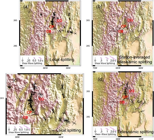
(a) Local and (b) station-averaged teleseismic (SKS, SKKS and PKS) shear wave splitting results (black lines) plotted at the stations that recorded the respective seismic phase. (c) Zoom in for the Cerro Galán ignimbrite complex shown in (a). (d) 115 teleseismic shear wave splitting measurements after quality control. Cerro Galan (CG), Carachi Pampa (CP) and Cerro Blanco (CB) volcanic centres are shown for reference. Average local lag time is 0.5 s and average teleseismic lag time is 2 s.
The local splitting events displayed in Figs 3(a) and (c) show a much more complex pattern both in fast direction orientations and lag times averaging 0.58 s. A rotation pattern of fast directions around Cerro Galan is not clear. However, approximately trench parallel fast directions towards the west of the array can be observed. The lag times drop to less than 0.4 s to the southeast of the Cerro Galan region where the slab shallows. Significant differences in fast directions at the same station from different sources (paths) are suggested to be indicative of the 3-D anisotropic structure beneath the southern Puna plateau.
3 SHEAR WAVE SPLITTING TOMOGRAPHY
3.1 Method
Shear wave splitting is generally characterized by good lateral resolution with very poor vertical resolution (Savage 1999). Although it is possible to get an idea of the depth of anisotropy by direct comparison between the lag times of teleseismic and local events, a tomographic inversion can be done in order to determine a 3-D anisotropic structure. We performed a tomographic inversion using a recently developed method that has been used to resolve the 3-D anisotropic structure beneath Nicaragua and Costa Rica (Abt & Fischer 2008; Abt et al.2009). The inversion assumes a mantle composed of 70 per cent olivine and 30 per cent orthopyroxene. Experimentally determined elastic constants, pressure and temperature derivatives for olivine are also considered. At crustal depths the inversion continues to assume mantle mineralogy since the crustal lag times are smaller than teleseismic lag times and local lag times. The 0.2 s average crustal splitting lag time is time is assumed to be the average lag time measured from events within the range 100–120 km depth divided by two since the average crustal thickness is around 55 km. Hence, crustal shear wave splitting lag times would be smaller than the average local event splitting lag times of 0.58 s and are not likely to cause significant differences when making the above simplification. In addition, crustal anisotropy is much more complex and varies over much smaller length scales than the size of our tomographic models (i.e. 50 km blocks).
Using the orthorhombic symmetry of both minerals we set the LPO such that the ‘a’-axis of olivine is parallel to the ‘c’-axis of orthopyroxene, and the ‘b’-axis of olivine is parallel to the ‘a’-axis of orthopyroxene. We assume the ‘c’-axis of olivine to be horizontal yielding a hexagonal symmetry defined solely by two angles: θ (azimuth of the [1 0 0] axis) and ψ (dip of the [1 0 0] axis), which simplifies the problem and the interpretations. The degree of anisotropy is controlled by a parameter ‘α’ called the strength parameter, which varies from 0 to 100 per cent. This strength parameter reduces the effect of anisotropy on the predicted delay time in each model block relative to that from its single crystal value. Hence, our model vector is defined by the combination of the three parameters θ, ψ and α.
The forward calculation of predicted shear wave splitting parameters (φ, dt) is done using the approximate particle motion perturbation method of Fischer et al. (2000) which allows for 3-D distributions and orientations of anisotropy. The effects of anisotropy in each block along a ray path are calculated by progressively rotating and time-shifting the horizontal components of a simple wavelet that has an initially linear particle motion. We use initial polarizations estimated from our local events shear wave splitting observations that were estimated using a grid search algorithm that minimizes the energy in the radial component.
For the inversion we investigated starting models in which the distribution of anisotropy parameters is uniform, random and based on averaging of our shear wave splitting measurements. In an average starting model, the orientation and strength of anisotropy were obtained by averaging the splitting parameters that sample the block, weighting them by their path lengths in the block. We settled on the average starting models presented here, as they show the smallest residuals (differences between observed splitting parameters and those predicted by the best-fitting model) considering our station-earthquake distribution. Abt & Fischer (2008) also reported smaller residuals in Central America with an average starting model.
In order to determine the seismic anisotropy beneath and within the subducting Nazca lithosphere, we include teleseismic shear wave splitting measurements. We assume that these teleseismic phases integrate anisotropy from 400 km depth to the surface. This is a common assumption and is based on the observation that splitting fast directions are similar regardless of propagation direction, which indicates that the region below the upper mantle is fairly isotropic (Silver & Chan 1991; Savage 1999; Niu & Perez 2004). In addition, other studies have also found the mantle transition zone to be approximately isotropic (Vinnik et al.1992, 1995, 1996; Barruol & Mainprice 1993; Mainprice & Silver 1993) and the lower mantle is generally regarded as being isotropic. While this is likely to be true beneath ocean basins, it may not be necessarily the case in subduction zones (Long & Becker 2010). Specifically, the base of the lower mantle, D″, is believed to exhibit both azimuthal and polarization anisotropy (Yamazaki & Karato 2007; Lynner & Long 2012) and the lower mantle beneath Southern America is no exception (Vanacore & Niu 2011).
Using this approach, we considered a set of virtual hypocentres for a given teleseismic event. The number of virtual hypocentres depends upon the number of stations that recorded a particular event. We calculated the angles at which the rays reached 400 km depth and then back projected the location of the virtual hypocentres with respect to each station down to 400 km. Because the teleseismic rays are close to being vertical and very few of them cross, anisotropy within and below the slab cannot be separately resolved, and only average anisotropy is estimated at these depths.
We used a linearized damped least-squares inversion (Tarantola 1987) to find the best fitting model of anisotropy (θ, ψ and α: crystallographic orientation and strength of fabric alignment combination). This was done by minimizing the misfit between the observed and predicted shear wave splitting parameters. The G matrix (the matrix of partial derivatives used in the inversion) was numerically calculated by varying model parameters and measuring the resulting changes in predicted splitting parameters (fast direction and lag time). The G matrix was recalculated when the model parameters changed by more than 1 degree (in the case of θ, ψ) or 1 per cent (in the case of α) between iterations. We also weighted the data using their errors, which are obtained from the 95 per cent confidence contour by taking the maximum separation in the fast direction and lag time axis, respectively. In order to keep the changes in model parameters small enough that the linear partial derivatives are valid during all iterations, we damped the inversion. A total of 100 iterations and 503 km3 size blocks were used. We ran inversions using the using only the 115 teleseismic rays containing our best shear wave splitting results (results not shown here), using 441 local rays (not shown here) and using a combination of local and teleseismic shear wave splitting measurements with a total of 556 rays.
3.2 Resolution
3.2.1 Resolution matrix
One of the advantages of the matrix inversion technique is that it provides a direct way to calculate the resolution of the model parameters. Plots of the resolution matrix in the supporting information show the diagonal values of the model resolution matrix for the three model parameters: the strength of anisotropy (α), azimuth (θ) and dip (ψ). As expected, the highest resolution tends to be concentrated at the shallower depths and around the stations. For depths 50–200 km, the region of good resolution tends to move towards the epicentres of the local events, north and south of the array. For depths below 200 km we observe some isolated regions of high resolution centred on virtual epicentres of the teleseismic events. In general, the resolution is higher for the azimuth and lower for the dip. In the case of the dip, there are no regions of good resolution beneath 150 km as there are few crossing rays at those depths. Overall, the resolution is fairly good at the depth range 0–100 km, which is where most of the rays cross.
3.2.2 Checkerboard test
Using the distribution of local event and teleseismic paths in the real dataset, we tested model resolution using a checkerboard test. Fig. 4(a) shows the input checkerboard model of a-axes orientations with alternating horizontal east–west and north–south orientations in blocks of 1003 km3. Figs 4(b)–(e) show the models obtained from an average starting model after 100 iterations at depth ranges of 0–100, 100–200, 200–300 and 300–400 km; only the blocks sampled by phase paths are shown. The recovery of the input model is best in the 0–100 km layer within the blocks spanned by the stations. Recovery decreases with increasing depth as expected from the resolution matrix results.
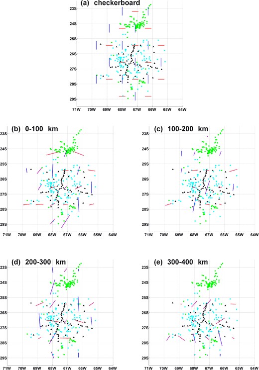
(a) Checkerboard with east–west (red lines) and north–south (blue lines) a-axes with block sizes of 100 km. This pattern repeats for every depth up to 400 km. Local seismicity is shown as green dots and teleseismic pseudo-epicentres are shown as cyan dots. The stations are represented by black triangles. (b) Checkerboard results for depths 0–100 km, (c) 100–200 km, (d) 200–300 km and (e) 300–400 km. Overall the checkerboard is roughly recovered with resolution decreasing with increasing depth.
Fig. 5 shows the difference between checkerboard a-axes orientations and inverted orientations using synthetic shear waves and the real station and event distribution for depth ranges of 0–100, 100–200, 200–300 and 300–400 km. The fit is good (blue) for regions covering the stations and local events for depths of 0–300 km (Figs 5a–c) but decreases as depth increases. Regions of good fit cover part of the station array but not the local events at depths of 300–400 km.
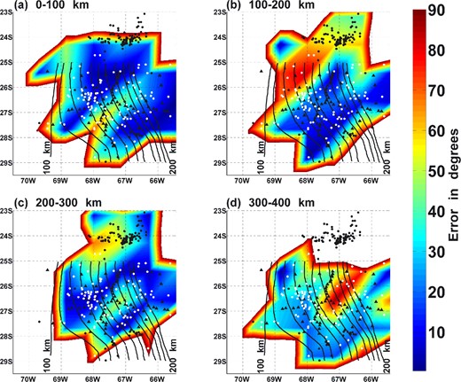
Difference between checkerboard a-axis azimuths and inverted azimuths using synthetic shear waves and the real seismic station and earthquake distribution for depth ranges of (a) 0–100 km, (b) 100–200 km, (c) 200–300 km and (d) 300–400 km. The seismic stations are shown as black triangles, local events as black dots and pseudo teleseismic epicentres as white dots. The slab contours (Mulcahy et al.2014) for depths 100–200 km in intervals of 10 km are shown as black solid lines.
Fig. 6 shows the difference between checkerboard strength of anisotropy values and inverted strength of anisotropy values using synthetic shear wave and the real station-event distribution for ranges of 0–100, 100–200, 200–300 and 300–400 km. In this case, we only observe good fit (blue regions) for depths of 0–100 km (Fig. 6a) that covers most of the stations and part of the region where the local events are originated.
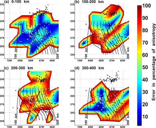
Difference between checkerboard strength of anisotropy values and inverted strength of anisotropy values using synthetic shear waves and the real seismic station and earthquake distribution for depth ranges of (a) 0–100 km, (b) 100–200 km, (c) 200–300 km and (d) 300–400 km. The seismic stations are shown as black triangles, local events as black dots and pseudo teleseismic epicentres as white dots. The slab contours (Mulcahy et al.2014) for depths 100–200 km in intervals of 10 km are shown as black solid lines.
3.3 Shear wave splitting tomography results
Figs 7 and 8 show the results when using 556 ray paths in the inversion, which combines 115 teleseismic ray paths with 441 local shear wave splitting measurements. The blue and red lines’ orientation and length represent the a-axes orientation and strength of anisotropy, respectively. The blue lines are more closely oriented north-south, and the red lines are more closely oriented east–west. Fig. 7 shows the views of a-axes and strength of anisotropy for 0–100, 100–200, 200–300 and 300–400 km depth slices. Beneath the western part of the array, we observe a-axes mainly oriented parallel to the trench and exhibiting a slight change to a northeast direction with increasing depth. On average, the strength of anisotropy decreases towards the west of the array, where the mantle wedge thins. At depths of less than 200 km (Figs 7a and b), a rotation of the a-axes beneath Cerro Galan and Cerro Blanco occurs, and in some cases they transition to an east–west direction. At greater depths (see Figs 7c and d), there is evidence for both trench parallel and trench orthogonal a-axes orientations throughout the southern Puna plateau with some complexities around Cerro Galan. Interestingly, the results beneath Cerro Galan show that the strength of anisotropy is smaller than that of adjacent regions (Figs 7c and d). Fig. 8 shows the results versus depth as viewed from the south and west of the seismic station array. Fig. 8 shows that the slab and subslab anisotropy tend to be mainly horizontal and that there is a region in the mantle wedge (depth range of 50–100 km) between longitudes 66.8° W and 68° W, and latitudes 25.5° S and 27° S (beneath Cerro Blanco, Carachi Pampa and the west part of Cerro Galan) with evidence of vertical a-axes. It is important to mention that these are better resolved than those in prior inversions using only local splitting measurements or only teleseismic splitting measurements. We have examined the resolution of jointly inverting both observations and found that the resolution degrades when only using local shear wave splitting data or teleseismic shear wave splitting data.
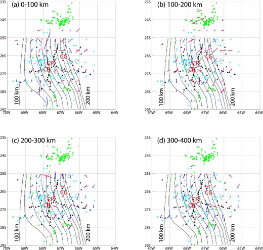
Map view of shear wave splitting tomography with 556 (teleseismic and local earthquake) rays for various depth ranges. The blue and red lines’ orientation and length represent the a-axis orientation and strength of anisotropy, respectively. The blue lines are most closely oriented north–south, and the red lines are most closely oriented east–west. Slab contours for 100–200 km depth in 10 km increments are shown in black thin lines (Mulcahy et al.2014). The local events are shown as green dots and the teleseismic events as cyan dots. The stations are shown as black triangles. At depths of 0–100 and 100–200 km there is a rotational pattern around Cerro Galan (CG) that also involves Cerro Blanco (CB) and Carachi Pampa (CP) volcanic centres. Below the slab (200–300 km and 300–400 km depth) There is evidence for both trench parallel and trench orthogonal a-axis orientations (blue and red lines) throughout the region except beneath Cerro Galan where the strength of anisotropy decreases significantly and the rotational pattern is not clear.

(a) Across longitude and (b) across latitude view of the shear wave splitting tomography results with 556 (teleseismic and local earthquake) rays. The blue and red lines’ orientation and length represent the a-axis orientation and strength of anisotropy, respectively. The blue lines are most closely oriented north–south, and the red lines are most closely oriented east–west. The slab contours are shown as black lines (Mulcahy et al.2014). Local seismicity is shown as green dots and teleseismic pseudo epicentres are shown as cyan dots at 400 km depth. There is some evidence for close to vertical a-axes beneath Cerro Galan and Cerro Blanco ignimbrite complexes. The a-axes are mostly horizontal below the slab.
4 DISCUSSION
Subduction zones where the slab dip has varied rapidly through time are likely to lead to complex mantle flow and seismic anisotropy and thus complex patterns of shear wave splitting fast directions and delay times (Druken et al.2011; Long 2013). The southern Puna region offers a mantle wedge with such complex anisotropic patterns due to the change in subduction angle from normal to the north to flat south of 27°S (Mulcahy et al.2014), episodes of crustal and lithospheric delamination with upwelling of hot asthenosphere (Kay & Coira 2009; Calixto et al.2013), and a heated slab or, possibly, a slab gap associated with a gap of intermediate depth seismicity (Calixto et al.2013; Mulcahy et al.2014). The recent episodes of delamination started around 6 Ma with the most recent large delamination event at around 2 Ma (e.g. Kay & Coira 2009) possibly triggered by slab roll back. Cerro Galan is associated with a high velocity-low attenuation body (delaminated crust and lithosphere) at around 140 km depth beneath the northern edge of Cerro Galan (Bianchi et al.2013; Calixto et al.2013; Liang et al.2014), with widespread crustal melting and an abnormally heated slab (possibly a slab gap) beneath the southwestern edge of Cerro Galan. The region has also been subjected to an evolving stress regime with a change from a mainly NW–SE compressive regime during most of the Miocene to a more chaotic regime after the latest Miocene (e.g. Marrett et al.1994; Risse et al.2008; Mulcahy et al.2014).
Given that the region where delamination is observed (west of 68W) might reveal totally different patterns than other regions, we have decided to divide the following part of the discussion into two sections outlining the patterns observed west and east of 68W instead of the usual mantle wedge, slab and subslab division. Sections 4.1 and 4.2 assume that the time for LPO to develop is smaller than the time over which the geometry of strain changes along the flow-lines, so that the olivine a-axes align close to the direction of flow. This may not necessarily be true for the mantle wedge but the observation of different flow patterns in different parts of the mantle wedge is still valid although the a-axes orientations may not be parallel to the flow.
4.1 West of 68W
The western stations of the Puna array seem to follow a trench parallel alignment of fast directions both in local and teleseismic shear wave splitting measurements (Fig. 3). This is also seen in the tomographic inversion at depths of 0–100 and 100–200 km (Figs 7a and b) with mostly trench parallel a-axes and a slight rotation to northeast orientation for depths below 200 km (Figs 7c and d). At depths above 130 km this pattern is most likely not related to mantle wedge corner flow (Behn et al.2007; Long 2013) or 3-D flow around the slab (Long & Silver 2008) as the slab depth in this region is around 100–120 km and there is probably little to no mantle wedge since the lithosphere thickness is around 100–130 km in the southern Puna (Calixto et al.2013). Moreover, Fig. 7 shows no major variation in the strength of anisotropy (length of lines in Fig. 7) with respect to depth west of 68W, which agrees with the mantle wedge not significantly contributing to the seismic anisotropy in this region. Thus, this pattern is interpreted as splitting produced by horizontal shortening of the continental lithosphere and slab caused by the compressive regime due to the collision of the Nazca and South American plates.
At subslab depths (Figs 7c and d), the observed trench parallel pattern may reflect anisotropy beneath the slab as affected by slab rollback (Long & Silver 2009; Long 2013) which causes trench orthogonal flow due to the retreating or steepening slab in the mantle wedge above the slab but trench parallel flow beneath the retreating or steepening slab. This is in agreement with other studies in subduction zones showing subslab trench parallel fast directions (Vinnik et al.1992; Russo & Silver 1994; Yu & Park 1994; Kaneshima & Silver 1995; Gledhill & Stuart 1996; Gledhill & Gubbins 1996; Long & Silver 2008; Abt et al.2010; MacDougall et al.2012). The central Andes have a history of trench migration or change subduction angle (Kay & Coira 2009) which may have lead to a significant amount of subslab anisotropy and likely trench parallel splitting (Long & Silver 2008).
The fact that the a-axes at depths below the slab (see west of 68W in Figs 7c and d) show a slight rotation to the east might indicate a slight, though not significant, coupling of the subslab mantle with the subducting slab (Paczkowski 2012; Long 2013). This slight rotation could also be an indicator of roll back being the dominant mechanism driving the flow in the subslab area. There are mainly two mechanisms of flow acting at subslab depths, namely roll back and the downward motion of the subducting plate (Faccenda & Capitanio 2012), that tend to produce trench parallel and trench perpendicular fast direction patterns, respectively. However, the observation that most subslab a-axes in the western part the array are either trench parallel or slightly rotated to the east suggest that the stronger mechanism driving the flow in this subslab area is linked to slab roll back and that the effect of plate advance, or downward motion of the Nazca plate, is less significant. Subduction dip angle, normal in the north and flat in the south, could also be another factor accounting for the non-trench parallel component a-axes in the subslab region as it may cause pressure gradients as the slab subducts.
The consistent subslab trench parallel a-axes orientations across the western part of the array (west of 68W) suggest that the inversion assumption that all anisotropy is contained in the upper 400 km is a good approximation and that most subslab anisotropy is generated near the slab affected mostly by slab roll back and by a simple shear mechanism. However, some percentage of anisotropy could be also contained below 400 km. One example is the D″ layer beneath South America (Vanacore & Niu 2011) which may produce both shape preferred orientation (SPO) and LPO (Yamazaki & Karato 2007). The large Fresnel zones for lower mantle sources of anisotropy (Alsina & Snieder 1995) would limit the resolution at those depths. Resolution of shear wave splitting parameters is already low at depths of 300–400 km (see Figs S1–S3). Therefore, this study does not attempt to perform tomographic inversions below 400 km.
4.2 East of 68W
The region east of 68W shows a totally different pattern of seismic anisotropy including more complicated patterns both in local and teleseismic splitting results (Fig. 3) with mixed evidence for trench parallel and trench perpendicular fast direction. Interestingly, this is sometimes also observed in splitting measurements seen at the same stations (Fig. 3a), which is consistent with a 3-D anisotropic fabric. The region around the volcanic centres of Cerro Galan, Cerro Blanco and Carachi Pampa seems to exhibit a rotation of fast directions in local splittings (Fig. 7a) and is less pronounced in teleseismic splittings which show a reduction in lag times to an average of 1 second as compared to the ∼2 s regional average. The complexity of the patterns is also seen in the splitting tomography results (Fig. 7) where there seems to be a transition from trench parallel to trench orthogonal a-axes towards the east for at depths of 0–100 and 100–200 km.
At depths of 0–100 km (Fig. 7a), the pattern just east of 68W most likely still reflects the compression of the lithosphere but it rapidly changes eastward beneath the Cerro Galan ignimbrite, where the inferred delamination of a 50 thick high velocity block and subsequent upwelling of hot asthenosphere (Bianchi et al.2013; Calixto et al.2013; Liang et al.2014) is likely to be the predominant mechanism driving the flow. In this region, the lithosphere is significantly thinner and the patterns start to reflect flow that at some point reached the surface and resulted in the generation of large amounts of crustal melt. The lower crust in this part of the southern Puna is slow and partially molten as shown by shear wave velocity models (Calixto et al.2013) and by the blocked high frequency local S-waves travelling beneath Cerro Galan (Liang et al.2014; Mulcahy et al.2014). Figs 8(a) and (b) shows some evidence for near vertical a-axes beneath the Cerro Galan, Cerro Blanco and Carachi Pampa volcanic regions at depths of 50–100 km. Importantly, these are all regions where dip resolution is fairly good (see Fig. 3S). These near vertical fast directions are interpreted to indicate post-delamination asthenospheric upwelling, (Calixto et al.2013), and manifested by volcanic complexes at the surface. There is no other evidence for fast directions being aligned vertically or close to vertical anywhere else in our model.
At depths of 100–200 km, Fig. 8 shows only horizontal a-axes orientations. It is important to note that the dip resolution at depths below 100 km is very poor (see Fig. 3S) and it is very unlikely that the inversion could resolve any vertical flow. Fig. 7(b) shows some trench orthogonal a-axes (red lines) just east of 68W and also a very abrupt change in inferred a-axes orientations over short distances. This might be due to the fact that at these depths we are seeing a combination of anisotropy from the slab, subslab and also the mantle wedge (see slab contours in Fig. 7b). In addition, the presence of a heated slab or, possibly, a slab gap beneath the western edge of Cerro Galan at 25.5–26.0S could also influence the patterns observed. The recent delamination events could have imposed a rapid regional change of flow causing a less coherent flow field and a weak LPO (Long & Silver 2008).
South of 27S and east of 68W (i.e. southeast of the Cerro Galan region) the local splitting lag times drop to less than 0.4 s (Fig. 3a). This is also observed in Fig. 8(b) as a decrease in the strength of anisotropy. This region is characterized by shallow subduction angle and thus, the observations could be linked to a southward thinning of the mantle wedge rather than to changes in the mantle flow regime.
At subslab depths of 200–300 km and 300–400 km and east of 68W, the a-axes are mostly horizontal (Fig. 8) and there is evidence for both trench parallel and trench orthogonal a-axes throughout the region (Figs 7c and d). In particular, there seems to be a rotational pattern around Cerro Galan that can be seen from 25S to 28S at depths of 200–300 km (Fig. 7c) and it is not as clear at depths below 300 km (Fig. 7d). In addition, it is also observed that the region just east of Cerro Galan and the eastern edge of Cerro Galan (region between 67W-68W and 25.5S-26.5S) shows significantly reduced strength of anisotropy (length of lines in Fig. 7). This is consistent with the teleseismic lag times for the stations in this region (Fig. 3b). This region of less seismic anisotropy is directly beneath the region where a hot slab or, possibly, a slab gap is observed (Calixto et al.2013). The large rotational pattern observed around the region with small lag times can be interpreted as indirect evidence suggesting vertical flow through a slab gap. Even if we assume no slab gap, the inferred hotter slab (based on Qs and Vs) could locally influence the subslab flow south of Cerro Galan and possibly account for this pattern. North and south of Cerro Galan, the dominant mantle flow driving mechanism seems to be roll back and the effect of the heated slab is producing small rotations in the a-axes (Fig. 7c). The area beneath 300 km is not in direct contact with the slab and therefore the rotational pattern is not expected to be as clear. At these depths, roll back also seems to overcome the effect of the heated slab north and south of Cerro Galan, where nearly trench parallel a-axes are observed (blue lines in Fig. 7d). The fact that the inferred vertical a-axes beneath 200 km are not observed in the shear wave splitting tomography results (Fig. 8) can probably be attributed to the lack of dip resolution at these depths (see Fig. S3).
5 CONCLUSIONS
A complex pattern of shear wave splitting under the southern Puna is the product of the 3-D anisotropic structure resulting from distinct LPO regimes in the subslab mantle, the slab, the mantle wedge and the lithosphere. In addition, delamination, a partially heated slab and a change in slab subduction angle also play important roles in regionally changing the patterns of seismic anisotropy. Combining teleseismic and local shear wave splitting measurements aides in estimating the depth extent and 3-D anisotropy beneath and within the slab as well as improving the resolution in the mantle wedge. Overall, there is probably a significant amount of anisotropy beneath and possibly within the slab. The lithosphere west of 68W tends to produce trench parallel fast directions and inferred a-axes, which may be attributed to the compression and deformation of the Southern America plate. The dominant mechanism in the subslab mantle west of 68W seems to be slab rollback and a slight coupling between the subducting Nazca plate and the underlying mantle. This makes the subslab region west of 68W exhibit mainly trench parallel a-axes with slight trench orthogonal components. The deformation in the mantle wedge (east of 68W) is controlled by plate motion and also, regionally, by delamination and a heated slab (or slab gap) making the shear wave splitting patterns more complex and variable over relatively small length scales. Some evidence for close to vertical a-axes seems to suggest vertical flow beneath the main non-arc volcanic centres of the region and just west of the recently imaged delaminated block (Calixto et al.2013). The subslab mantle deformation and flow east of 68W and north and south of the Cerro Galan region appears to be mostly driven by slab roll back, whereas the inferred mantle flow beneath Cerro Galan seems to be controlled by a heated subducting slab or possible slab gap. This explains the observed rotational pattern centred on a region with small anisotropy strength and small lag times. This is considered to be an indirect evidence for vertical flow through a slab gap.
It is important to mention that we have our best resolution above the slab, where most of the rays (teleseismic and locals) cross, but not beneath or within the slab, where few teleseismic rays cross and no local rays are present; therefore, in such a region we are just estimating the average bulk anisotropic parameters.
We are grateful to two anonymous reviewers for their outstanding comments and suggestions that contributed to greatly improve the manuscript. This work was funded by NSF grant proposal EAR-0538245.
REFERENCES
SUPPORTING INFORMATION
Additional Supporting Information may be found in the online version of this article:
Figure S1. Resolution of the strength of azimuthal anisotropy for depth intervals of 50 km from 0 to 400 km. The resolution is shown as coloured contours. The seismic stations are shown as black triangles.
Figure S2. Resolution of the azimuth of the [1 0 0] axis for depth intervals of 50 km from 0 to 400 km. The resolution is shown as coloured contours. The seismic stations are shown as black triangles.
Figure S3. Resolution of the dip of the [1 0 0] axis for depth intervals of 50 km from 0 to 400 km. The resolution is shown as coloured contours. The seismic stations are shown as black triangles.
Figure S4. Teleseismic events (black dots) used in the study. They originate from a variety of azimuths.
Figure S5. Local events used in the study (black dots). The read triangles represent the location of the Puna network seismic stations.
Please note: Oxford University Press is not responsible for the content or functionality of any supporting materials supplied by the authors. Any queries (other than missing material) should be directed to the corresponding author for the article.
