SMART layers: a simple and robust alternative to PML approaches for elastodynamics Free

Non-zero eigenvalues and their corresponding eigenvector of |$\mathbf{\tilde{A}}_x$|⁠.

Eigenvalues	Eigenvectors
\|$e_{x_P}^+=\alpha$\|	\|$\vec{\mathbf {v}}_{x_P}^+=\left[1 \quad 0 \quad {-}(\lambda +\mu )/\alpha \quad {-}\mu /\alpha \quad 0 \right]^T$\|
\|$e_{x_P}^-=-\alpha$\|	\|$\vec{\mathbf {v}}_{x_P}^-=\left[1 \quad 0 \quad (\lambda +\mu )/\alpha \quad \mu /\alpha \quad 0 \right]^T$\|
\|$e_{x_S}^+=\beta$\|	\|$\vec{\mathbf {v}}_{x_S}^+=\left[0 \quad {-}\beta /\mu \quad 0 \quad 0 \quad 1 \right]^T$\|
\|$e_{x_S}^-=-\beta$\|	\|$\vec{\mathbf {v}}_{x_S}^-=\left[0 \quad \beta /\mu \quad 0 \quad 0 \quad 1\right]^T$\|

Eigenvalues	Eigenvectors
\|$e_{x_P}^+=\alpha$\|	\|$\vec{\mathbf {v}}_{x_P}^+=\left[1 \quad 0 \quad {-}(\lambda +\mu )/\alpha \quad {-}\mu /\alpha \quad 0 \right]^T$\|
\|$e_{x_P}^-=-\alpha$\|	\|$\vec{\mathbf {v}}_{x_P}^-=\left[1 \quad 0 \quad (\lambda +\mu )/\alpha \quad \mu /\alpha \quad 0 \right]^T$\|
\|$e_{x_S}^+=\beta$\|	\|$\vec{\mathbf {v}}_{x_S}^+=\left[0 \quad {-}\beta /\mu \quad 0 \quad 0 \quad 1 \right]^T$\|
\|$e_{x_S}^-=-\beta$\|	\|$\vec{\mathbf {v}}_{x_S}^-=\left[0 \quad \beta /\mu \quad 0 \quad 0 \quad 1\right]^T$\|

Table 1.

Non-zero eigenvalues and their corresponding eigenvector of |$\mathbf{\tilde{A}}_x$|⁠.

Eigenvalues	Eigenvectors
\|$e_{x_P}^+=\alpha$\|	\|$\vec{\mathbf {v}}_{x_P}^+=\left[1 \quad 0 \quad {-}(\lambda +\mu )/\alpha \quad {-}\mu /\alpha \quad 0 \right]^T$\|
\|$e_{x_P}^-=-\alpha$\|	\|$\vec{\mathbf {v}}_{x_P}^-=\left[1 \quad 0 \quad (\lambda +\mu )/\alpha \quad \mu /\alpha \quad 0 \right]^T$\|
\|$e_{x_S}^+=\beta$\|	\|$\vec{\mathbf {v}}_{x_S}^+=\left[0 \quad {-}\beta /\mu \quad 0 \quad 0 \quad 1 \right]^T$\|
\|$e_{x_S}^-=-\beta$\|	\|$\vec{\mathbf {v}}_{x_S}^-=\left[0 \quad \beta /\mu \quad 0 \quad 0 \quad 1\right]^T$\|

Eigenvalues	Eigenvectors
\|$e_{x_P}^+=\alpha$\|	\|$\vec{\mathbf {v}}_{x_P}^+=\left[1 \quad 0 \quad {-}(\lambda +\mu )/\alpha \quad {-}\mu /\alpha \quad 0 \right]^T$\|
\|$e_{x_P}^-=-\alpha$\|	\|$\vec{\mathbf {v}}_{x_P}^-=\left[1 \quad 0 \quad (\lambda +\mu )/\alpha \quad \mu /\alpha \quad 0 \right]^T$\|
\|$e_{x_S}^+=\beta$\|	\|$\vec{\mathbf {v}}_{x_S}^+=\left[0 \quad {-}\beta /\mu \quad 0 \quad 0 \quad 1 \right]^T$\|
\|$e_{x_S}^-=-\beta$\|	\|$\vec{\mathbf {v}}_{x_S}^-=\left[0 \quad \beta /\mu \quad 0 \quad 0 \quad 1\right]^T$\|

Table 2.

Non-zero eigenvalues and their corresponding eigenvector of |$\mathbf{\tilde{A}}_y$|⁠.

Eigenvalues	Eigenvectors
\|$e_{y_P}^+=\alpha$\|	$\vec{\mathbf {v}}_{y_P}^+=\left[\begin{array}{ccccc}0 \quad 1 \quad -(\lambda +\mu )/\alpha \quad \mu /\alpha \quad 0 \end{array}\right]^T$
\|$e_{y_P}^-=-\alpha$\|	$\vec{\mathbf {v}}_{y_P}^-=\left[\begin{array}{ccccc}0 \quad 1 \quad (\lambda +\mu )/\alpha \quad -\mu /\alpha \quad 0 \end{array}\right]^T$
\|$e_{y_S}^+=\beta$\|	$\vec{\mathbf {v}}_{y_S}^+=\left[\begin{array}{ccccc}-\beta /\mu \quad 0 \quad 0 \quad 0 \quad 1 \end{array}\right]^T$
\|$e_{y_S}^-=-\beta$\|	$\vec{\mathbf {v}}_{y_S}^-=\left[\begin{array}{ccccc}\beta /\mu \quad 0 \quad 0 \quad 0 \quad 1 \end{array}\right]^T$

Eigenvalues	Eigenvectors
\|$e_{y_P}^+=\alpha$\|	$\vec{\mathbf {v}}_{y_P}^+=\left[\begin{array}{ccccc}0 \quad 1 \quad -(\lambda +\mu )/\alpha \quad \mu /\alpha \quad 0 \end{array}\right]^T$
\|$e_{y_P}^-=-\alpha$\|	$\vec{\mathbf {v}}_{y_P}^-=\left[\begin{array}{ccccc}0 \quad 1 \quad (\lambda +\mu )/\alpha \quad -\mu /\alpha \quad 0 \end{array}\right]^T$
\|$e_{y_S}^+=\beta$\|	$\vec{\mathbf {v}}_{y_S}^+=\left[\begin{array}{ccccc}-\beta /\mu \quad 0 \quad 0 \quad 0 \quad 1 \end{array}\right]^T$
\|$e_{y_S}^-=-\beta$\|	$\vec{\mathbf {v}}_{y_S}^-=\left[\begin{array}{ccccc}\beta /\mu \quad 0 \quad 0 \quad 0 \quad 1 \end{array}\right]^T$

Table 2.

Open in new tab Download slide

Non-zero eigenvalues and their corresponding eigenvector of |$\mathbf{\tilde{A}}_y$|⁠.

Eigenvalues	Eigenvectors
\|$e_{y_P}^+=\alpha$\|	$\vec{\mathbf {v}}_{y_P}^+=\left[\begin{array}{ccccc}0 \quad 1 \quad -(\lambda +\mu )/\alpha \quad \mu /\alpha \quad 0 \end{array}\right]^T$
\|$e_{y_P}^-=-\alpha$\|	$\vec{\mathbf {v}}_{y_P}^-=\left[\begin{array}{ccccc}0 \quad 1 \quad (\lambda +\mu )/\alpha \quad -\mu /\alpha \quad 0 \end{array}\right]^T$
\|$e_{y_S}^+=\beta$\|	$\vec{\mathbf {v}}_{y_S}^+=\left[\begin{array}{ccccc}-\beta /\mu \quad 0 \quad 0 \quad 0 \quad 1 \end{array}\right]^T$
\|$e_{y_S}^-=-\beta$\|	$\vec{\mathbf {v}}_{y_S}^-=\left[\begin{array}{ccccc}\beta /\mu \quad 0 \quad 0 \quad 0 \quad 1 \end{array}\right]^T$

Eigenvalues	Eigenvectors
\|$e_{y_P}^+=\alpha$\|	$\vec{\mathbf {v}}_{y_P}^+=\left[\begin{array}{ccccc}0 \quad 1 \quad -(\lambda +\mu )/\alpha \quad \mu /\alpha \quad 0 \end{array}\right]^T$
\|$e_{y_P}^-=-\alpha$\|	$\vec{\mathbf {v}}_{y_P}^-=\left[\begin{array}{ccccc}0 \quad 1 \quad (\lambda +\mu )/\alpha \quad -\mu /\alpha \quad 0 \end{array}\right]^T$
\|$e_{y_S}^+=\beta$\|	$\vec{\mathbf {v}}_{y_S}^+=\left[\begin{array}{ccccc}-\beta /\mu \quad 0 \quad 0 \quad 0 \quad 1 \end{array}\right]^T$
\|$e_{y_S}^-=-\beta$\|	$\vec{\mathbf {v}}_{y_S}^-=\left[\begin{array}{ccccc}\beta /\mu \quad 0 \quad 0 \quad 0 \quad 1 \end{array}\right]^T$

Non-zero eigenvalues in Tables 1 and 2 correspond to P- and S-waves travelling in positive and negative direction over the x- and y-coordinates for |$\mathbf {\tilde{A}}_x$| and |$\mathbf {\tilde{A}}_y$|⁠, respectively. Since each of them has multiplicity 1, the projectors for each eigenvalue can be computed as

\begin{equation} \begin{array}{ccc}\mathbf {B}_{\theta _P}^\pm =\frac{\vec{\mathbf {v}}_{\theta _P}^\pm (\vec{\mathbf {v}}_{\theta _P}^\pm )^T}{\parallel \vec{\mathbf {v}}_{\theta _P}^\pm \parallel ^2}, &\quad \mathbf {B}_{\theta _S}^\pm =\frac{\vec{\mathbf {v}}_{\theta _S}^\pm (\vec{\mathbf {v}}_{\theta _S}^\pm )^T}{\parallel \vec{\mathbf {v}}_{\theta _S}^\pm \parallel ^2}, &\quad \forall \theta \in \lbrace x,y\rbrace . \end{array} \end{equation}

(16)

The SMART term |$\mathbf {B}(\vec{\mathbf {x}})$| is a linear combination of these projectors weighted by damping coefficients |$d_{\theta }^\pm$| such that

\begin{equation} \mathbf {B}(\vec{\mathbf {x}})=\sum _{\theta \in \lbrace x,y\rbrace }d_\theta ^+(\vec{\mathbf {x}})\sum _{\gamma \in \lbrace P,S\rbrace }B_{\theta _\gamma }^++ \sum _{\theta \in \lbrace x,y\rbrace }d_\theta ^-(\vec{\mathbf {x}})\sum _{\gamma \in \lbrace P,S\rbrace }B_{\theta _\gamma }^-. \end{equation}

(17)

The damping coefficients |$d_{\theta }^\pm (\vec{\mathbf {x}})$| are smooth mono-dimensional functions which are zero in the domain of interest and have a polynomial growth inside the layers.

As well as Etienne et al. (2010), we choose the damping profile proposed by Collino & Tsogka (2001) for PMLs such that

\begin{equation} d_{\theta }^\pm (\vec{\mathbf {x}})=d_{\theta _{\rm max}}^\pm \left(\frac{\delta _\theta ^\pm (\vec{\mathbf {x}})}{L_{\rm smart}}\right)^2\qquad \forall \theta \in \lbrace x,y\rbrace , \end{equation}

(18)

with

\begin{equation} d_{\theta _{\rm max}}^\pm =-3\alpha \frac{\log (R_{\rm coeff})}{2L_{\rm smart}}\qquad \forall \theta \in \lbrace x,y\rbrace , \end{equation}

(19)

where |$\delta _\theta ^\pm (\vec{\mathbf {x}})$| is the depth inside the SMART layers in the θ coordinate, L_smart is the SMART layer thickness and R_coeff is the theoretical reflection coefficient.

Following Halpern et al. (2011), adding the SMART term B, eq. (17), in the general hyperbolic system, eq. (9), leads to the equation

\begin{equation} \mathbf {S}\partial _t\vec{\mathbf {u}}+\sum _{\theta \in \lbrace x,y\rbrace }\mathbf {A}_{\theta }\partial _{\theta }\vec{\mathbf {u}} + \mathbf {S}\mathbf {B}\vec{\mathbf {u}} = \vec{\mathbf {g}}, \end{equation}

(20)

Since we would rather work with the velocity-stress formulation given in eqs (1) and (2), we split the damping term Z = SB from eq. (20) into

\begin{equation} \mathbf {Z}=\left[\begin{array}{cc}\mathbf {D} &\quad \mathbf {E} \\ \mathbf {G} &\quad \mathbf {H} \end{array}\right], \end{equation}

(21)

with

\begin{eqnarray} \begin{array}{cc}\mathbf {D}=\left[\begin{array}{cc}z_{1,1} &\quad z_{1,2} \\ z_{2,1} &\quad z_{2,2} \end{array}\right] &\quad \mathbf {E}=\left[\begin{array}{ccc}z_{1,3} &\quad z_{1,4} &\quad z_{1,5} \\ z_{2,3} &\quad z_{2,4} & z_{2,5} \end{array}\right] \\ \mathbf {G}=\left[\begin{array}{cc}z_{3,1} &\quad z_{3,2} \\ z_{4,1} &\quad z_{4,2} \\ z_{5,1} &\quad z_{5,2} \end{array}\right] &\quad \mathbf {H}=\left[\begin{array}{ccc}z_{3,3} &\quad z_{3,4} &\quad z_{3,5} \\ z_{4,3} &\quad z_{4,4} &\quad z_{4,5} \\ z_{5,3} &\quad z_{5,4} &\quad z_{5,5} \end{array}\right]. \end{array} \end{eqnarray}

(22)

We thus incorporate the SMART term in our velocity–stress formulation, eqs (1) and (2), as

\begin{eqnarray} \rho \partial _t\vec{\mathbf {v}}&=&\sum _{\theta \in \lbrace x,y\rbrace }\partial _\theta \mathbf {M}_\theta \vec{\mathbf {\sigma }} -\mathbf {D}\vec{\mathbf {v}}-\mathbf {E}\vec{\mathbf {\sigma }}+ \vec{\mathbf {f}} \end{eqnarray}

(23)

\begin{eqnarray} \mathbf {C}\partial _t\vec{\mathbf {\sigma }}&=&\sum _{\theta \in \lbrace x,y\rbrace }\partial _\theta \mathbf {N}_\theta \vec{\mathbf {v}} -\mathbf {H}\vec{\mathbf {\sigma }}-\mathbf {G}\vec{\mathbf {v}}. \end{eqnarray}

(24)

We shall turn our attention how to solve this new system, eqs (23) and (24), by a DGM.

2.2 Discontinuous Galerkin method

To solve the hyperbolic system, eqs (23) and (24), we first decompose the domain Ω into K elements, such that

\begin{equation} \Omega \simeq \Omega _h=\sum _{i=1}^KD_i, \end{equation}

(25)

where each D_i is a straight-sided triangle. The sum of the triangles form the mesh which has to be geometrically conforming. Following Etienne et al. (2010) we apply a nodal DGM to the weak formulation of eqs (23) and (24) to obtain

\begin{eqnarray} &&{\rho _i(\mathbf {I}_2\otimes \mathbf {K}_i)\frac{\vec{\mathbf {v}}_i^{n+\frac{1}{2}}-\vec{\mathbf {v}}_i^{n-\frac{1}{2}}}{\Delta t}}\nonumber\\ &&\!=-\sum _{\theta \in \lbrace x,y\rbrace }(\mathbf {M}_\theta \otimes \mathbf {E}_{i_\theta })\vec{\mathbf {\sigma }}_i^n+\sum _{k\in N_i}\left[(\mathbf {P}_{ik}\otimes \mathbf {F}_{ik})\frac{\vec{\mathbf {\sigma }}_i^n+\vec{\mathbf {\sigma }}_k^n}{2}\right] \nonumber\\ &&\!- (\mathbf {D}_i\otimes \mathbf {K}_i)\vec{\mathbf {v}}_i^n-(\mathbf {E}_i\otimes \mathbf {K}_i)\vec{\mathbf {\sigma }}_i^n+(\mathbf {I}_2\otimes \mathbf {K}_i)\vec{\mathbf {f}}_i^{n+\frac{1}{2}} \end{eqnarray}

(26)

\begin{eqnarray} &&{(\mathbf {C}_i\otimes \mathbf {K}_i)\frac{\vec{\mathbf {\sigma }}_i^{n+1}-\vec{\mathbf {\sigma }}_i^n}{\Delta t}}\nonumber\\ &&\!= -\sum _{\theta \in \lbrace x,y\rbrace }(\mathbf {N}_\theta \otimes \mathbf {E}_{i_\theta })\vec{\mathbf {v}}_i^{n+\frac{1}{2}}+ \sum _{k\in N_i}\left[(\mathbf {Q}_{ik}\otimes \mathbf {F}_{ik})\frac{\vec{\mathbf {v}}_i^{n+\frac{1}{2}}+\vec{\mathbf {v}}_k^{n+\frac{1}{2}}}{2}\right] \nonumber \\ &&\!-(\mathbf {H}_i\otimes \mathbf {K}_i)\vec{\mathbf {\sigma }}_i^{n+\frac{1}{2}}-(\mathbf {G}_i\otimes \mathbf {K}_i) \vec{\mathbf {v}}_i^{n+\frac{1}{2}}. \end{eqnarray}

(27)

In eqs (26) and (27), ⊗ represent the tensor product, N_i is the group of adjacent elements to the i-triangle and the superscript n indicates the time step. The involved matrices are the mass matrix, K_i, the stiffness matrices, |$\mathbf {E}_{i_\theta }$|⁠, for all θ ∈ {x, y}, the flux matrix, F_ik and the auxiliary flux matrices, |$\mathbf{P}_{ik}$| and |$\mathbf{Q}_{ik}$|⁠. The definitions of these matrices can be found, in Etienne et al. (2010) or Tago et al. (2012). The SMART matrices, D_i, E_i, H_i and G_i depends on the position and physical properties of the i-triangle.

The proposed DGM, eqs (26) and (27), uses a second-order explicit leap-frog scheme for the time integration and a centred scheme for the fluxes evaluation. The combination of this two makes the DGM energy conservative, efficient and easy to program. However more sophisticated DGM schemes have been successfully proposed, as the ADER-DG proposed by Käser & Dumbser (2006) who uses a modal representation, upwind fluxes and the ADER time integration approach.

The incorporation of the SMART layers makes the right-hand-side (RHS) term of the velocity scheme, eq. (26), dependent not only on the stresses but also on the velocities. The leap-frog scheme requires the velocities computed at the n-time, |$\vec{\mathbf {v}}_i^n$|⁠. A simple approximation is

\begin{eqnarray} \vec{\mathbf {v}}_i^n=\frac{1}{2}\left(\vec{\mathbf {v}}_i^{n+\frac{1}{2}}+\ \vec{\mathbf {v}}_i^{n-\frac{1}{2}}\right). \end{eqnarray}

(28)

This simple choice makes the time integration semi-implicit. However, because of the local nature of DGM, we can invert the involved small local matrices to recover an explicit time integration through the following:

\begin{eqnarray} &&{\left[\left(\mathbf {I}_2\otimes \mathbf {I}_{\rm dof}\right)+\frac{\Delta t}{2\rho _i}\left(\mathbf {D}\otimes \mathbf {I}_{\rm dof}\right)\right]\vec{\mathbf {v}}_i^{n+\frac{1}{2}}}\nonumber \\ &&\!=\vec{\mathbf {v}}_i^{n-\frac{1}{2}}+\frac{\Delta t}{\rho _i}(\mathbf {I}_2\otimes \mathbf {K}_i)^{-1}\vec{\mathbf {r}}_i^n \nonumber\\ &&\!-\frac{\Delta t}{2\rho _i}(\mathbf {D}_i\otimes \mathbf {I}_{\rm dof})\vec{\mathbf {v}}_i^{n-\frac{1}{2}}-\frac{\Delta t}{\rho _i}(\mathbf {E}_i\otimes \mathbf {I}_{\rm dof})\vec{\mathbf {\sigma }}_i^n, \end{eqnarray}

(29)

where the subscript dof stands for the degrees of freedom inside the i-triangle and

\begin{equation} \vec{\mathbf {r}}_i^n=-\sum _{\theta \in \lbrace x,y\rbrace }(\mathbf {M}_\theta \otimes \mathbf {E}_{i_\theta })\vec{\mathbf {\sigma }}_i^n+\sum _{k\in N_i}\left[(\mathbf {P}_{ik}\otimes \mathbf {F}_{ik})\frac{\vec{\mathbf {\sigma }}_i^n+\vec{\mathbf {\sigma }}_k^n}{2}\right]. \end{equation}

(30)

The treatment of the RHS of the stress scheme, eq. (27), follows the same path as the one done for the velocity scheme, eq. (26). The needed stress at the |$n+\frac{1}{2}$|-time is approximated with the expression

\begin{eqnarray} \vec{\mathbf {\sigma }}_i^{n+\frac{1}{2}}=\frac{1}{2}\left(\vec{\mathbf {\sigma }}_i^{n+1}+\vec{\mathbf {\sigma }}_i^n\right). \end{eqnarray}

(31)

The stress scheme, eq. (27), is transformed into the explicit time integration

\begin{eqnarray} &&{\left[(\mathbf {I}_3\otimes \mathbf {I}_{\rm dof})+\frac{\Delta t}{2}(\mathbf {C}_i^{-1}\mathbf {H}_i \otimes \mathbf {I}_{\rm dof})\right]\vec{\mathbf {\sigma }}_i^{n+1}}\nonumber\\ &&=\vec{\mathbf {\sigma }}_i^n+\Delta t(\mathbf {C}_i \otimes \mathbf {K}_i)^{-1}\vec{\mathbf {o}}_i^{n+\frac{1}{2}}-\frac{\Delta t}{2}(\mathbf {C}_i^{-1}\mathbf {H}_i\otimes \mathbf {I}_\mathrm{dof})\vec{\mathbf {\sigma }}_i^n \nonumber \\ &&-\Delta t(\mathbf {C}_i^{-1}\mathbf {G}_i\otimes \mathbf {I}_\mathrm{dof})\vec{\mathbf {v}}_i^{n+\frac{1}{2}}, \end{eqnarray}

(32)

with

\begin{eqnarray} \vec{\mathbf {o}}_i^{n+\frac{1}{2}}\!=\! -\!\sum _{\theta \in \lbrace x,y\rbrace }(\mathbf {N}_\theta \otimes \mathbf {E}_{i_\theta })\vec{\mathbf {v}}_i^{n+\frac{1}{2}} \!+\! \sum _{k\in N_i}\left[(\mathbf {Q}_{ik}\otimes \mathbf {F}_{ik})\frac{\vec{\mathbf {v}}_i^{n+\frac{1}{2}}+\vec{\mathbf {v}}_k^{n+\frac{1}{2}}}{2}\right].\nonumber\\ \end{eqnarray}

(33)

The simple approximations for |$\vec{\mathbf {v}}_i^n$| and |$\vec{\mathbf {\sigma }}_i^{n+\frac{1}{2}}$| degrade the convergence behaviour of the leap-frog scheme. Yet since the SMART matrices are different from zero only inside the SMART layers, the impact will be only in these zones.

3 NUMERICAL TEST

We perform the numerical comparison between the C-PML and SMART layers with a very simple model, where long-term C-PML instabilities appear with the DGM scheme. The C-PML implementation is done following the work of Etienne et al. (2010). The ordinary differential equations, related with the memory variables introduced, are solved with the same DGM scheme used to update the velocity–stress hyperbolic system. We consider an homogeneous half-space 10 000 m width and 5000 m depth with the physical parameters α = 4000 m s⁻¹, β = 2310 m s⁻¹ and ρ = 2000 kg m⁻³. The source is a Ricker pulse with a dominant frequency of 3 Hz located near the free surface at the middle of the domain x_s = 0 m and z_s = 10 m. The domain is discretized using a conforming unstructured triangular mesh. We used quadratic interpolation functions inside each triangle, P2 elements, so the mesh ensures three elements per minimum wavelength. The total simulation time is 30 s.

3.1 C-PML instabilities and SMART comparison

Absorbing boundary layers are defined at the two lateral sides and at the bottom of the domain. On top we apply a free surface boundary condition. The C-PMLs width is 10 elements, as proposed by Etienne et al. (2010) when using a DGM approach. The damping profile are the ones presented in Section 2. The Fig. 1 presents snapshots of v_x at different times of the simulation. We observe that the C-PMLs absorb effectively the outgoing waves. However, a strong amplification coming from the layer appears later. This can also be observed in Fig. 2(a) where we present seismograms for v_x and v_y obtained using receivers located along the free-surface at the same depth than the source.

Figure 1.

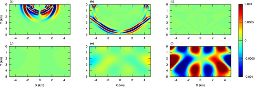
Snapshots of v_x while including 10-element width C-PMLs at both lateral sides and the bottom of the model at: (a) 1 s, (b) 2.4 s, (c) 5 s, (d) 15 s, (e) 25 s and (f) 30 s.

Figure 2.

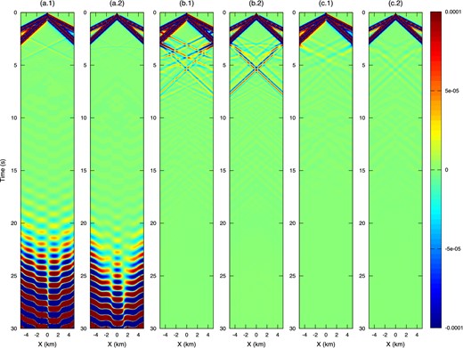
Seismograms of v_x and v_y for 10-elements C-CPML, (a.1) and (a.2), respectively, 10-elements SMART layers, (b.1) and (b.2), respectively, and 20-elements SMART layers, (c.1) and (c.2), respectively. The scale is saturated two orders below the average of the velocity wavefield to better distinguish the reflections.

Open in new tab Download slide

We reproduce this test using 10 elements SMART layers, keeping the same mesh and damping profile used for the C-PMLs. We show in Fig. 2(b) that the SMART layers do not suffer from the amplification phenomenon. However, the coupling between the simulation domain and the SMART layers is not as satisfactory as the one obtained with a C-PML. Particularly, for waves propagating at grazing angles, we observe stronger reflections at the interface between the domain of interest and the layer (from 3 to 8 s). In order to reduce the magnitude of the reflections at the order of magnitude of the C-PML reflections, we can increase the width of the SMART layers from 10 to 20 elements. The seismograms for 20 elements SMART layers are given in Fig. 2(c).

To prove the robust dissipative property of the SMART layers, we run the same configuration using 20 elements SMART layers but we increase the total simulation time from 30 to 300 s. In Fig. 3, we present the history of the kinematic energy. The decrease is very fast at the beginning of the simulation. After reaching several orders of magnitude below the magnitude of the wavefield propagated, it seems that the noise level is attained. The kinematic energy keeps being attenuated at a small rate. This emphasizes the dissipative property of the SMART layers.

Figure 3.

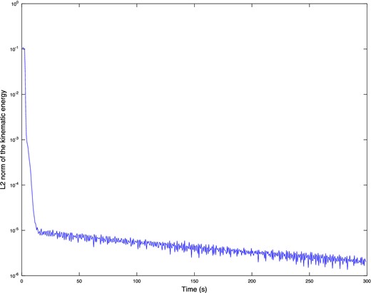
History of the L2 norm of the kinematic energy using 20-elements SMART layers which decreases with time until the noise level.

Open in new tab Download slide

The increase of the number of elements in the SMART layers makes the computation more expensive. This is necessary to reach the same level of accuracy than the one achieved with the C-PMLs. However, as can be seen in Table 3, an additional feature of the SMART layers method is that for a given width of the layer, it requires less memory and less Floating Point Operations (FLOP's) than C-PMLs. The data presented in Table 3 depend on our specific implementation. However, looking at the system eqs (23) and (24), it is clear that independently of the numerical scheme for a given absorbing layer width, SMART layers are cheaper in memory and time than C-PMLs because it only consists in the introduction of a zero-order term, and do not require additional memory variables with their respective ordinary differential equations. For our implementation, with 20 elements SMART layers (78.16 per cent SMART elements from the total of elements in the mesh), using Table 3, we can compute that they are approximately 1.1 more time consuming and 1.2 more memory expensive than 10 elements C-PMLs (36.32 per cent CPML elements from the total of elements in the mesh). This is the small price we have to pay to avoid the C-PML instabilities that, as can be seen in Figs 2(a), starts polluting the velocities fields a few seconds after the wavefield has reached the layers. These factors are even smaller when the ratio between the domain elements and absorbing boundary elements increases.

Table 3.

Memory and FLOP comparison between the C-PML and the SMART layers using P2 elements in our DGM implementation. The ‘Element’ columns consider the whole memory and FLOP's per P2 element inside the absorbing layer during an update step. While the ‘Abs. layer’ columns involve the memory and FLOP's required only by the absorbing layer operations by P2 element inside the absorbing layer during an update step.

	Memory (bytes)		FLOP
	Element	Abs. layer	Element	Abs. layer
C-PML	468	256	5073	2262
SMART	332	120	3141	330
C-PML/SMART	1.409	2.133	1.615	6.854

	Memory (bytes)		FLOP
	Element	Abs. layer	Element	Abs. layer
C-PML	468	256	5073	2262
SMART	332	120	3141	330
C-PML/SMART	1.409	2.133	1.615	6.854

Table 3.

Memory and FLOP comparison between the C-PML and the SMART layers using P2 elements in our DGM implementation. The ‘Element’ columns consider the whole memory and FLOP's per P2 element inside the absorbing layer during an update step. While the ‘Abs. layer’ columns involve the memory and FLOP's required only by the absorbing layer operations by P2 element inside the absorbing layer during an update step.

	Memory (bytes)		FLOP
	Element	Abs. layer	Element	Abs. layer
C-PML	468	256	5073	2262
SMART	332	120	3141	330
C-PML/SMART	1.409	2.133	1.615	6.854

	Memory (bytes)		FLOP
	Element	Abs. layer	Element	Abs. layer
C-PML	468	256	5073	2262
SMART	332	120	3141	330
C-PML/SMART	1.409	2.133	1.615	6.854

4 CONCLUSIONS AND PERSPECTIVES

The SMART layers is a robust alternative to PML approaches for elastodynamic simulations. They are easier to implement and for a given absorbing layer width faster than C-PMLs. We showed that they are robust in a case where C-PMLs are unstable. However, since the SMART layers are not perfectly matched, stronger reflections than those observed in the C-PML approach are generated. In order to increase the efficiency of the SMART layers to the same level of the C-PMLs, we had to double the width of the SMART layers. However, this only implies a small cost of time and memory in comparison with the C-PML approach, as the SMART layers only consist in introducing a zero-order term in the initial system.

For 3-D simulations, the SMART layers width enlargement would increment the ratio of SMART layers elements with respect to regular elements. Nonetheless, the gap of the element memory and FLOP's requirements between SMART and C-PMLs increases too. We believe that the sum of both effects would preserve the 2-D relative cost of the SMART layers for 3-D simulations. Furthermore, for anisotropic elastodynamic simulations, the SMART layers relative cost should be smaller than for isotropic elastodynamic simulations. The anisotropy implies cross-derivatives that would increase the amount of memory variables required by the C-PML strategy.

We believe that SMART layers could be very useful for long time 3-D elastodynamics simulations in regional scales for seismic hazard evaluation where C-PML instabilities could appear. Further studies to better match the SMART layers should be done to decrease the layer's width.

We thank Andreas Fichtner and Roland Martin for their remarks and suggestions. This work has been supported by the French Agence Nationale de la Recherche under the grant ANR-2011-BS56-017 and partially funded by sponsors of the SEISCOPE II consortium (http://seiscope2.osug.fr) and from the European Community's Seventh Framework Programme [FP7/2007-2013] under the grant agreement PEOPLE-2011-IRSES 295217.

REFERENCES

Ben Jemaa

M.

Glinsky-Olivier

N.

Cruz-Atienza

V.M.

Virieux

J.

Piperno

S.

,

Dynamic non-planar crack rupture by a finite volume method

,

Geophys. J. Int.

,

2007

, vol.

171

(pg.

271

-

285

)

Bérenger

J.-P.

,

A perfectly matched layer for absorption of electromagnetic waves

,

J. Comput. Phys.

,

1994

, vol.

114

(pg.

185

-

200

)

Burridge

R.

,

Elastic Waves in Anisotopric Media

,

1996

Schlumberger-Doll Research

Cerjan

C.

Kosloff

D.

Kosloff

R.

Reshef

M.

,

A nonreflecting boundary condition for discrete acoustic and elastic wave equations

,

Geophysics

,

1985

, vol.

50

4

(pg.

2117

-

2131

)

Chew

W.C.

Liu

Q.H.

,

Perfectly matched layers for elastodynamics: a new absorbing boundary condition

,

J. Comput. Acoust.

,

1996

, vol.

4

(pg.

341

-

359

)

Clayton

R.

Engquist

B.

,

Absorbing boundary conditions for acoustic and elastic wave equations

,

Bull. seism. Soc. Am.

,

1977

, vol.

67

(pg.

1529

-

1540

)

Collino

F.

,

High order absorbing boundary conditions for wave propagation models: straight line boundary and corner cases

,

Proceedings of the Second International Conference on Mathematical and Numerical Aspects of Wave Propagation

,

1993

Delaware

SIAM

(pg.

161

-

171

)

Google Preview

Collino

F.

Tsogka

C.

,

Application of the perfectly matched absorbing layer model to the linear elastodynamic problem in anisotropic heterogeneous media

,

Geophysics

,

2001

, vol.

66

(pg.

294

-

307

)

Dmitriev

M.M.

Lisitsa

V.V.

,

Application of M-PML reflectionless boundary conditions to the numerical simulation of wave propagation in anisotropic media. Part I: reflectivity

,

Numer. Anal. Appl.

,

2011

, vol.

4

(pg.

271

-

280

)

Etienne

V.

Chaljub

E.

Virieux

J.

Glinsky

N.

,

An hp-adaptive discontinuous Galerkin finite-element method for 3D elastic wave modelling

,

Geophys. J. Int.

,

2010

, vol.

183

2

(pg.

941

-

962

)

Halpern

L.

Petit-Bergez

S.

Rauch

J.

,

The analysis of matched layers

,

Confluentes Mathematici

,

2011

, vol.

3

2

(pg.

159

-

236

)

Hastings

F.D.

Schneider

J.B.

Broschat

S.L.

,

Application of the perfectly matched layer (PML) absorbing boundary condition to elastic wave propagation

,

J. acoust. Soc. Am.

,

1996

, vol.

100

(pg.

3061

-

3069

)

Käser

M.

Dumbser

M.

,

An arbitrary high order discontinuous Galerkin method for elastic waves on unstructured meshes I: the two-dimensional isotropic case with external source terms

,

Geophys. J. Int.

,

2006

, vol.

166

(pg.

855

-

877

)

Komatitsch

D.

Martin

R.

,

An unsplit convolutional perfectly matched layer improved at grazing incidence for the seismic wave equation

,

Geophysics

,

2007

, vol.

72

5

(pg.

SM155

-

SM167

)

Komatitsch

D.

Tromp

J.

,

A perfectly matched layer absorbing boundary condition for the second-order seismic wave equation

,

Geophys. J. Int.

,

2003

, vol.

154

1

(pg.

146

-

153

)

Martin

R.

Komatitsch

D.

Gedney

S.D.

,

A variational formulation of a stabilized unsplit convolutional perfectly matched layer for the isotropic or anisotropic seismic wave equation

,

Comput. Model. Eng. Sci.

,

2008

, vol.

37

(pg.

274

-

304

)

Métivier

L.

Brossier

R.

Labbé

S.

Operto

S.

Virieux

J.

,

A robust absorbing layer for anisotropic seismic wave modeling

,

J. Comput. Phys.

,

2014a

in press

Métivier

L.

Brossier

R.

Operto

S.

Virieux

J.

,

A robust absorbing layer method for seismic wave simulation in anisotropic media

,

Proceedings of the 76th Annual EAGE Meeting

,

2014b

Expanded Abstracts, Amsterdam

Google Preview

Métivier

L.

Brossier

R.

Operto

S.

Virieux

J.

,

Smart: Robust absorbing layer and s-waves filtering for acoustic anisotropic wave simulation

,

Proceedings of the 84th Annual SEG Meeting

,

2014c

Expanded Abstracts, Denver

Google Preview