Hybrid analysis of multiaxis electromagnetic data for discrimination of munitions and explosives of concern

Summary

1 Introduction

The remediation of land containing munitions and explosives of concern (MEC), also known as unexploded ordnance (UXO), is a problem facing the United States and other countries whose UXO-contaminated lands are being transferred to civilian use (Gasperikova & Beard 2007). Cleanup of UXO-contaminated lands using traditional methods based on detecting and excavating anomalous geophysical responses is prohibitively expensive. Furthermore, it is not sufficient to merely detect buried metal objects because many of these objects are not UXO and therefore pose no hazards. In many cleanup cases, 70per cent or more of the cost consists of locating and removing harmless metal objects including soda cans, broken parts from agricultural equipment and fragments of previously exploded ordnance (Bowers & Bidwell 1999). For these reasons, research is being directed in the United States and elsewhere to developing better geophysical systems for the detection and identification (discrimination) of buried UXO (McKenna & Pulsipher 2009). Detection is the identification of anomalous geophysical responses. Discrimination is being able to distinguish between dangerous UXO and harmless fragments of metallic clutter. Classification takes discrimination one step further by identifying the individual types of UXO that have been detected. Among the primary geophysical systems used to detect and classify UXO are time and frequency domain electromagnetic induction (McNeill & Bosnar 1996; Geng et al. 1999; Carin et al. 2001; Pasion & Oldenburg 2001; Zhang et al. 2003; Wright et al. 2006, 2008) and magnetics techniques (Nelson & McDonald 2001; Billings 2004).

Some challenges facing geophysicists during UXO cleanup operations are the development of improved system sensors and software (Gasperikova & Beard 2007; McKenna & Pulsipher 2009). Since the mid-1990s, geophysical sensors have continued to improve in their ability to detect conductive and permeable targets (Won et al. 1997; O'Neill et al. 2004; Huang et al. 2007). By contrast, data analysis software continues to require advancement in both pre- and post-processing stages. Examples of some pre-processing challenges involve not levelling data to such a degree that buried targets are removed from the analysed data set and also mitigation of required operator intervention for large sets of data that could take a long time to pre-process. Examples of some post-processing challenges involve the accurate discrimination of UXO among geological and/or anthropogenic noise. The current technology renders site remediation a slow, labour-intensive and inefficient process with a high false alarm rate (McKenna & Pulsipher 2009). A key requirement for cost-effective UXO cleanup operations is a near real-time data-processing scheme capable of recording and discriminating target responses with a minimum false alarm rate, no false negatives (i.e. misses) and no operator intervention.

Traditional discrimination schemes are based on the numerical inversion of measured responses using forward modelling algorithms. Forward algorithms focus on approximating the response of unexploded munitions by multiple orthogonal dipoles (Pasion & Oldenburg 2001; Grimm 2003; Smith et al. 2004), permeable and conductive spheroids (Bell et al. 2001; Gasperikova 2003; Smith et al. 2004; Smith & Morrison 2006), or one or more inductively-coupled current loops (Lamontagne et al. 1998; Asten & Duncan 2007). The numerical inversion of measured responses includes algorithms based on non-linear gradient (Barnett 1984), Bayesian estimation (Julier 1998), Kalman filtering (Jekeli & Lee 2007) and continuation (Benavides & Everett 2007) methods. Despite advances in numerical inverse procedures, practical applications often are limited to synthetic data or when applied to field data the false alarm rates remain unacceptably high (McKenna & Pulsipher 2009). For this reason, other non-traditional discrimination schemes have also been evaluated including algorithms based on electromagnetic induction (EMI) catalogues (Pasion et al. 2007), evolutionary strategies (Zhang 2008) and artificial neural networks (Hart et al. 2000; Szidarovsky et al. 2008; Benavides et al. 2009).

An artificial neural network analysis includes both supervised and unsupervised approaches. Examples of supervised artificial neural networks used in UXO discrimination include probabilistic neural networks (Hart et al. 2000) and multilayer perceptrons (Szidarovsky et al. 2008). Of these, the multilayer perceptron technique was shown to distinguish between UXO and metallic clutter with high accuracy when applied to a particular synthetic data set (Szidarovsky et al. 2008). According to the authors, however, achieving high accuracy requires an understanding of which target parameters are important and how their non-linear interaction affects the desired outcome. This statement highlights potential problems associated with the need to accurately specify the output layer of the neural network before performing UXO discrimination. One promising alternative that requires no a priori knowledge of underlying relations or designation of an output layer is the self-organizing map (SOM) technique, which is an unsupervised approach (Kohonen 2001).

The SOM is a vector quantization technique that uses a competitive learning algorithm to classify patterns in data (Kohonen 2001). Applications of the SOM in geophysics include classification of multiple reflections (Essenreiter et al. 2001), seismic velocities (Lin et al. 2002), seismic facies (Castro de Matos et al. 2007), volcanic tremors (Langer et al. 2009), seismic wavefields (Kohler et al. 2010), UXO responses (Benavides et al. 2009) and airborne electromagnetic and radiometric responses (Friedel in press). According to Benavides et al. (2009), buried non-overlapping target responses can be classified with good accuracy when evaluating the U-matrix (Ultsch 2003) of a SOM trained on Geonics EM63 field data. Unfortunately, they present no independent verification of the field performance; that is, the site used to acquire the data to train the SOM also is used to validate the classification. In our study, we test the efficacy of a new multiaxis electromagnetic induction data collection and software system, called ALLTEM, to discriminate among randomly buried and overlapping metallic clutter and inert MEC. This study differs from Benavides et al. (2009) in that the SOM is first trained and independently validated, using SOM calibration data acquired at one site with subsequent blind tests conducted at other sites. In addition to classifying the target response (direct- and indirect-fire UXO and metallic clutter), the SOM also is used to estimate target characteristics (depth, orientation, azimuth, weight). To our knowledge, this is the first study to use the SOM as an estimator of target characteristics and to perform an independent field validation of overlapping targets.

2 Alltem

2.1 Electromagnetic induction

The ALLTEM is a time-domain multitransmitter, multireceiver electromagnetic induction system (Fig. 1). There are three orthogonal transmitters powered sequentially resulting in 19 transmitter–receiver combinations. The largest receiver is a 1m vertical gradiometer whereas the rest of the receivers are 0.34m in diameter arranged so that gradients in three directions are acquired for each transmitter. This new system is named ALLTEM because one of the transmitter currents is on all the time. The system is novel in that the transmitting (Tx) loops are sequentially driven by a continuous triangle current waveform and the resulting electromagnetically induced target responses, measured as voltages, are processed in the time domain. The triangle response is theoretically equivalent to an integration of the voltage measured by a conventional EMI system that uses a rapid current turn-off. Practically, the use of a triangle-waveform results in smaller early-time voltages induced in the Rx loops reducing dynamic-range demands on the receiver analogue electronics and the digitizer. Another useful consequence is that ferrous and non-ferrous targets generate markedly different responses (Wright et al. 2005, 2006). ALLTEM obtains the advantages of triangle-wave excitation in a system whose dimensions, characteristics and geometry are appropriate to UXO applications.

Figure 1

The ALLTEM 1-m sensor cube. The Tx loops produce orthogonal magnetic fields in three directions (Hx, Hy, Hz). The top and bottom faces contain a 1-m square Rx loop around the perimeter and four 34-cm printed circuit-board Rx loops on 50-cm centres. Each vertical face has two 34-cm Rx loops to measure fields in the two horizontal directions (Hx and Hy). Because a transmitter is always on, opposite Rx loops are paired as gradiometers to cancel the primary field.

Open in new tabDownload slide

2.2 Electromagnetic data

The ALLTEM data used in this study are from surveys conducted at the UXO Standardized Test Site at the Aberdeen Proving Ground, near Aberdeen, Maryland (Fig. 2). The survey areas are designated as the calibration grid, the Blind Test grid and the Direct Fire and Indirect Fire areas. Data maps from the 1-m-vertical gradient receiver coil, the ZZM component, are shown in Figs 3a and b. The calibration grid contains buried targets for which information including identity, depth of burial, orientation and weight are provided. These inert munition items include 25 mm, 37 mm, 60 mm, 81 mm, 105M60, 105HEAT, 155 mm, and 2.75-in projectiles as well as metallic clutter including shrapnel. 8 lbs cannon balls are placed in the corners of the grid. A summary of these targets and their characteristics is presented in Table 1. Those targets used in the calibration process are presented in Table 2. The station spacing of data collected along traverses is 0.20m at a survey speed of 1.0m s^–1.

Figure 2

Layout of the standardized UXO test site at the Aberdeen Proving Ground, Maryland. The calibration grid (labelled ‘CAL’ in the figure), Blind Test grid and the Direct Fire and Indirect Fire areas were surveyed. North direction is aligned with vertical side of figure.

Open in new tabDownload slide

Figure 3

ALLTEM response over buried targets at the Aberdeen Proving grounds, Aberdeen, Maryland: (a) calibration grid, (b) Blind Test grid. Information about items in the calibration grid is provided for characterization purposes. Number denotes target and patch (delineated by circle around target) used in data processing.

Open in new tabDownload slide

Table 1

Excerpt of known ALLTEM reference inversions and signal decay times. Units are in metrer and milliseconds.

Open in new tabDownload slide

Table 2

List of calibration targets for ALLTEM data collection at Aberdeen proving grounds.

Open in new tabDownload slide

Pre-processing of ALLTEM data involves removing the system response and background signature from the recorded waveforms, applying lowpass and bandpass filters, merging GPS information (which is converted from latitude–longitude to UTM easting–northing) with the waveforms, averaging the bipolar waveforms (1111 samples are reduced to 555 samples), integrating the area under waveforms to produce an indicator of composition (ferrous, non-ferrous or mixed) and exporting the data in a form suitable for input to Geosoft's Oasis Montaj program that is useful for database management and data analysis (Wright et al. 2005). ASCII files are created for each receiver polarization that include the line number, record number, easting, northing and 15 amplitudes (volts) at selected times of 10, 70, 220, 310, 450, 600, 750, 1050, 1350, 1850, 2500, 3500, 4500, 5130 and 5350μs with time zero being the onset time of the positive ramp of the 90-Hz-triangular transmitter current waveform.

The analysis tools developed for Oasis Montaj facilitate importing the pre-processed data and applying minimum-curvature gridding algorithms to the data (Wright et al. 2005). During the gridding, noise and statistics of background signal levels are computed based on a target free area to determine target locations and to set target thresholds. Filters are applied to sharpen the estimate of target location and then algorithms within Oasis Montaj are used to automatically select target locations within all 19 ALLTEM receiver data sets. Polygons are automatically created around each inferred target location using the statistics calculated earlier of the background signal levels. The area inside a polygon is called an anomaly patch. The data within each anomaly patch, in ASCII format, are then copied to individual subdirectories within the Oasis project directory. A typical ASCII file includes the target azimuth, inclination, time decay constant, weight, amplitudes at 15 time samples along the response decay curve and finally differences in amplitude between an early time sample (usually 310μs) and each of the succeeding time samples recorded. Eleven amplitude differences are calculated including the differences in amplitudes between the sample at time 310μs and at time 450, 310 and 600, 310 and 750μs and so on out to a difference between 310 and 5350μs. These data are ready for use in hybrid classification based on data-driven and numerical methods. A similar set of ASCII data files containing only the measured responses are used for the validation of the classification analyses.

3 Methods

3.1 Data-driven discrimination

3.1.1 Training

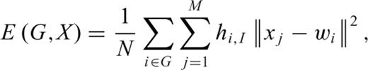
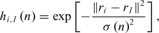
The data-driven discrimination of buried targets involves a three-step process: training of the SOM, estimation of target characteristics by the trained SOM and discrimination based on histograms of estimated target characteristics. In the training step, the SOM learns how to project the multidimensional data input layer onto a low-dimensional discrete lattice of N competitive neurons called the map. In this study, each input data item x ∈ X is a vector in the set X = [x₁,…, x_M]^T of dimension M. A fixed number of k neurons indexed to i is arranged on a regular grid G with each neuron associated to weight vectors w ∈ W in the set W = [w_i, … w_N]_T, which has the same dimensionality as an input vector. These weight vectors connect each input vector x in parallel to all neurons of G. The neurons are connected to each other, and in our case this interconnection is defined using a toroid topology.

The process of mapping is facilitated using a cost function E(G, X) defined as the weighted Euclidian norm given by

1

where h is the Gaussian neighbourhood function, and I is the best matching unit (BMU) vector. Evaluating the Euclidian norm for each input vector x_j requires calculating distances ‖x_j−w_i‖ over the grid to determine which weight vector is the closest to the input vector. The neuron with the closest weight vector is the winning neuron (BMU), with map coordinates (I_i,I_j), given by

2

and defines the central position of a neighbourhood function h_i,I. The neighbourhood function determines the contribution of each vector difference ‖x_j−w_i‖ to the total cost function and measured with respect to the current BMU. In this study, the neighbourhood function is defined as a Gaussian function given by

3

where ‖r_i−r_I‖ corresponds to the distance between neuron r_i and I in the map grid and σ (n) defines the width of the neighbourhood function, a monotonically decreasing function of the iteration (sometimes called epoch) number n. The position of the BMU also determines the neighbourhood centre and hence which subsets of neurons learn the most about the input vector.

In the second step, an updated weight is determined as a function of the distance to the current BMU expressed through the neighbourhood function. The weight update vector is given by

4

where a(n) is a scalar value called the learning rate that is bounded on the interval [0,1]. The BMU ensures that the largest weight update occurs at the BMU and is parallel to the input vector. The weight updating also takes place at the neighbouring nodes but to a lesser degree because of the Gaussian shape. The updating procedure causes the weight vectors of the BMU and its topological neighbours to resemble the input vector. Presenting similar input vectors to the map provokes further response in the same neighbourhood and thereby tends to produce clustering of data in the feature space. Association between neurons decreases during the learning process [the width of the neighbourhood function σ(n)² is forced to decrease] with n preserving large clusters of data whereas enabling the separation of other clusters that are closely spaced.

The SOM learning method that we use is the stochastic gradient described by Kohonen (1984). It consists of a two-step process that is performed each time an input pattern is presented to the map: competition to determine the BMU and cooperative learning (spreading information contained in the current input vector across the map). At the beginning of the unsupervised training phase, the weight vectors are initialized to small random numbers. The input data vectors X are then presented to the map grid in a random sequence to generate data clusters without introducing bias for a specific class. Each time that an input vector is presented to the map grid, the cost function is calculated and the number of times each neuron becomes is the BMU is recorded. At the end of each iteration, the average cost function R(E_n, X) is calculated using

5

where E_n are the n cost function realizations. The training process stops when R(E_n, X) is smaller than a prescribed fraction of its initial value; for example R(E_n, X) <10⁻⁵. Ultimately, this training process results in a topology where similarities among data patterns are mapped into similar weights of the neighbouring neurons, and the asymptotic local density function of the neural weights approach that of the training set (Ritter & Schulten 1986).

Before SOM training, the 65 456 records representing various ALLTEM traverses over selected subsurface targets at the calibration grid are split into two groups: group one for training (32 728 records) and group two for validation (32 728 records). In each group, there are 39 total variables. After excluding non-essential record variables, there are 34 active variables comprising 114 5480 discrete samples (data values). The active variables (name is in parentheses) include: target characteristics such as type (item), azimuth with respect to north (azim), depth (depth), inclination with respect to the horizontal surface (inclin) and weight (weight); and EMI dimensionless decay constant (alpha), time constantμs (tau); EMI amplitudes (volts) at time 10μs (T0), 70μs (T7), 220μs (T22), 310μs (T31), 450μs (T45), 600μs (T60), 750μs (T75), 1050μs (T105), 1350μs (T135), 1850μs (T185), 2500μs (T250), 3500μs (T350), 4500μs (T450), 5130μs (T513), 5350μs (T535); EMI gradients between times 310 and 450μs (31M45), 310 and 600μs (31M60), 310 and 750μs (31M75), 310 and 1050μs (31M105), 310 and 1350μs (31M135), 310 and 1850μs (31M185), 310 and 2500μs (31M250), 310 and 3500μs (31M350), 310 and 4500μs (31M450), 310 and 5130μs (31M513) and 310 and 5350μs (31M535). The data associated with these active variables are log transformed and randomly assigned (presenting the input vectors to the map sequentially using a randomly sorted database) as an initial set of map weight vectors. One reason for the transformation is to linearize data so that one value does not dominate the Euclidean distance metric (Vesanto & Alhoniemi 2000).

Application of the SOM to this training data is performed using a fixed number of neurons and topological relations. Specifically, the selected map topology is a toroid (wraps from top to bottom and side to side) with hexagonal neurons whose number is established based on the ratio between eigenvalues of the training data (Adaptive Informatics Research Center 2010). This rule-of-thumb provides the minimum number of neurons along map coordinates to facilitate separation of data vectors during their projection onto the map dimensions. Using this approach results in 54 rows (along its length) and 48 columns (along its width) for a total of 2784 neurons (about 2.5 times the square root of number of training samples). Training of the map is conducted in two phases: first rough and then fine. The rough training involves 20 iterations using a Gaussian neighbourhood with an initial and final radius of 73 units and 19 units; and the fine training involves 400 iterations using a Gaussian neighbourhood with a rough-scale and fine-scale radius of 19 units and 1 unit. The initial and final learning rates of 0.5 and 0.05 decay linearly down to 10⁻⁵, and the width of the Gaussian neighbourhood function decreases exponentially (at a decay rate of 10⁻³ iteration⁻¹) providing convergence for the UXO discrimination problem. The respective CPU times associated with rough and fine learning phases are about 5 min and 1 hr using a 2.66 GHz DuoCore Intel processor.

3.1.2 Target characteristic estimation and discrimination

Next, the trained SOM is used to simultaneously estimate target characteristics (azimuth, depth, inclination, item and weight) from all test site records based on distances among the available model vectors (Junninen et al. 2004; Kalteh & Berndtsson 2008; Kalteh & Hjorth 2009). In the traditional approach, estimates of target characteristics are taken directly from the weight vectors of the BMUs (Fessant & Midenet 2002; Wang 2003). However, certain training data sets result in biased estimates (Dickson & Giblin 2007; Malek et al. 2008) requiring a modified scheme that incorporates bootstrapping (Breiman 1996), ensemble average (Rallo et al. 2002) or nearest neighbour (Malek et al. 2008) approaches. This study uses an alternative iterative estimation scheme that minimizes the topographic error vector across the map of neurons (Fraser & Dickson 2007). Because of uncertainty in the training and estimation processes, separate histograms are created for each target parameter based on all of the records from the respective patch. The comparison among histograms provides a visual means for target discrimination of UXO.

3.2 Numerical discrimination

3.2.1 Forward model

The ALLTEM inversion uses the Biot–Savart law to model both the primary magnetic fields from the transmitter coils and those secondary magnetic fields, using reciprocity, generated by eddy currents induced in the target materials in the ground (West et al. 1984). The target response is currently modelled by three orthogonal dipoles from prolate and oblate spheroids with one major axis and two minor axes and by triaxial ellipsoids in which all three axes are different. The equivalent ellipsoid that models the ALLTEM response is embedded in a conductive, magnetic and optionally, a viscous magnetic Earth. The integral expressions for the magnetic fields generated by vertical magnetic dipoles and horizontal magnetic dipoles within a conductive magnetic half-space are given by Ward & Hohmann (1988). The ground response at a given receiver coil because of excitation by a given transmitter coil is calculated by numerically evaluating the following integrals,

6

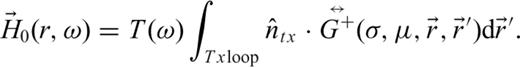
where T(ω) is the Fourier transform of the transmitter excitation (a triangle wave), is the dyadic Green's function for a receiver located above the surface because of a dipole moment also located above the surface, σ is the ground conductivity, μ is ground magnetic permeability (possibly complex and frequency dependent), ω is radian frequency, V_Rx is the voltage at the receiver coil, and are the normals to the planes containing the transmitting and receiving coils and the integrals are over the area of the transmitting and receiving coils with r and r' being the distances to the transmitter and receiver coils from a single point. This procedure is used to calculate the voltage at each receiving coil in the gradiometer, and then the difference is found between these coil voltages. Finally, the frequency-domain coil voltage difference is converted into a time-domain signal using a fast Fourier transformFFT.

Modelling the response of a conductive permeable ellipsoid is slightly more involved. First, the magnetic field below the surface is calculated at the centre of the target using eq. (7). Here the dyadic Green's function is for a receiver located below the surface because of a dipole moment located above the surface.

7

Next, the equivalent induced dipole moment for the target is calculated,

8

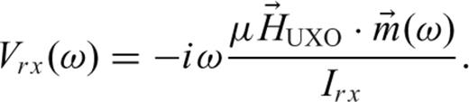
where is a diagonal frequency-dependent magnetic-polarizability tensor. Calculations of this tensor for conductive permeable prolate and oblate spheroids are given in Smith & Morrison (2006). A rotation matrix, , converts the magnetic field to target-centric coordinates. Note that for a given incident field, only a single component of the polarizability tensor is excited. A fully polarimetric instrument, like the ALLTEM, switches through different coil configurations resulting in incident fields with components in all possible directions at the location of the instrument. The result is that all components of the transmitted polarizability tensor are excited, which provides more information about the target.

The final step is to calculate the fields at a receiver coil because of the induced dipole moment at a target. Using the reciprocity theorem, we find that the voltage induced in a receiver coil V_Rx because of an induced target dipole moment is related to the magnetic field at the target because of a current in the receiver coil I_Rx by

9

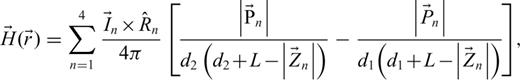
Eq. (7) is used to calculate the magnetic field at the target, only now the integral is over the area of the receiver coil. As before, this procedure is used to calculate the voltage at each receiving coil in the gradiometer, and the difference is found between these coil voltages. Finally the frequency-domain coil voltage is converted into a time-domain signal using a FFT.

Using eqs (6)–(9), and Smith & Morrison's (2006) spheroid response, the ALLTEM response to the Earth and the target are modelled separately, and then summed to determine the total response. The mutual inductance between the target and surrounding medium is neglected (i.e. the Born approximation). The magnetostatic response because of induced magnetization of a permeable target by the ALLTEM is manifest as a pulsed square wave response, with the decaying electromagnetic response because of induced eddy currents superimposed. The square wave magnetostatic response is absent for a non-permeable target. Note also that the electromagnetic eddy current decay lasts longer for the permeable target.

We model the induced magnetization as a linear problem (ignoring hysteresis and other non-linearities) that includes demagnetization based on the shape of the target. In practice, this approach is warranted because the magnetic field strengths are rather small (much less than saturated magnetic fields for steel) and the response is repeatable. Induced magnetization can add to the non-ferrous or a ferrous eddy current response. The demagnetization can also have a large effect (Oden 2012 and Smith & Morrison 2006) as well as viscous magnetization at locations such as Hawaii and Montana where basalts and associated weathered soil products contain significant amounts of iron.

When estimating parameters from large amounts of data, it is desirable to have a fast inversion algorithm, which in turn requires a fast forward model. Calculating the Green's function in eqs (6) and (7) is computationally expensive, and is not needed is many cases. A faster approach to calculating the magnetic fields is to use the static Biot–Savart law for free space. This works well for the ALLTEM system because all coils have a square shape, which simplifies the circuital integral using Biot–Savart. 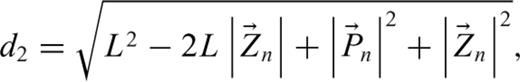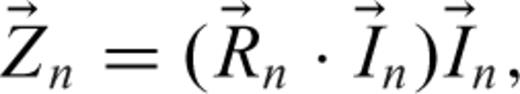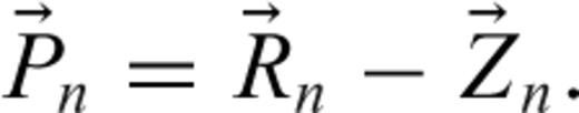The magnetic field at is the sum of the fields produced by the four straight wire segments, each with current , length 2L, and centred at , the midpoint of the wire segment (Jackson 1975):

10

11

12

13

14

15

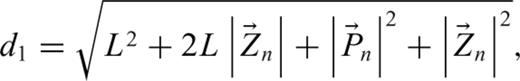
Smith et al. (2004) present a simple parametric form for estimating the time-domain B field response of a conductive permeable sphere because of a step function excitation.

This B-field response (B =μH) is also the electrodynamic ALLTEM response, because its excitation is an integral of a step (triangle wave), it uses dB/dt receivers, and the integral and derivative operations cancel (Smith & Annan 1998). The parametric step response of Smith et al. (2004) is a good approximation to the early-time, intermediate-time and late-time portions of the ALLTEM response. The simple models for permeable and non-permeable spheres reduce to (μ_r being the magnetic permeability of the target):

16

17

18

19

20

21

22

23

We combine this form with Smith & Morrison's (2006) approximation of the polarizability tensor for a prolate spheroid in terms of a sphere. For the nth element along the diagonal, this yields,

24

25

where b is the half-length (half the major axis) of the spheroid, a is the radius (half the minor axis) and the demagnetization factors A_n are given in Smith & Morrison (2006) eqs A.2 and A.3. The magnetostatic response is simply

26

Combining both the electrodynamic and the magnetostatic responses, we obtain

27

where the electrodynamic response at 5.55ms is subtracted to account for eddy currents that have not decayed when the transmitted waveform changes slope. Subtracting the magnetostatic response removes the ground response. Finally, the time-domain ALLTEM response is calculated from eqs (8), (9) and (27) where ω is replaced by t.

3.2.2 Inverse model

The inverse modelling algorithm employs an iterative Gauss–Newton minimization combined with step-size optimization as follows,

28

29

30

31

where is the pseudo-inverse of , and is the forward model vector containing predicted data samples, is the measured data, is a diagonal matrix containing the data standard deviations (assuming that the data are identically distributed and statistically independent), and contains the parameters (x_i is the model parameter vector at the ith iteration).

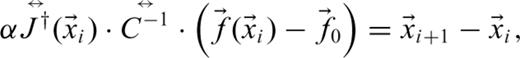
At each iteration, the step length is scaled by α in discrete steps over the interval [0,1] to find the step that minimizes the least-squares data misfit. Because the number of data (number of coil combinations times number of instrument locations times number of sampled waveform points) far exceeds the number of model parameters to be estimated for target characterization, the pseudo-inverse of the Jacobian matrix is calculated by singular-value decomposition. Instabilities because of poor conditioning are avoided by scaling the model parameters and by rejecting small singular values. The iterations stop when a local minimum is found, or the maximum allowable number of iterations is reached.

The first step in the parameter estimation problem of the inversion algorithm is to choose an initial model. The x and y target locations are selected based on the centroid of the anomaly, and the z location is then estimated by finding the least-squares minimum of

32

where f^c is the modelled data and f^c₀ is the measured data for coil combination c at instrument location n. All data are from the same late time-gate (usually t = 5ms), and ρ_n is the horizontal distance from the anomaly centroid to instrument location n.

The formula (32) calculates slopes of the logarithm of the fields versus distance from the target (i.e. slope is −3 for the fields of a static dipole decaying at r⁻³), and compares the slopes of measured and modelled data to that of a spheroid response. To determine a representative permeability value, the late-time magnitudes are examined, which differ if the target is ferrous or non-ferrous (μ_r = 1). For ferrous targets, the demagnetization effect must also be considered. For targets with relative permeabilities ranging from 50 to 1000 (Telford et al. 1990), a nominal value of 100 is sufficient to model ferrous UXO-type objects; therefore, the selected representative value of μ_r is held fixed during the inversion. An initial conductivity is chosen on based values of typical metals used in UXO construction. The conductivity of aluminium alloys typically range from about 1.5 × 10⁷ to 3.5 × 10⁷ S m^–1, and steel alloys typically range from 0.2 × 10⁷ to 0.9 × 10⁷ S m^–1, which makes 1.0 × 10⁷ S m^–1 a reasonable starting value (Telford et al. 1990). Initial orientation angles (pitch and yaw) are set to zero. With a representative permeability value, it is possible to determine the principal spheroid axes lengths using the response at time t = 0⁺ (the instant the transmitter turns off). However, this requires a system with instantaneous turn-off time and a receiver with infinite bandwidth. With some high-bandwidth systems, it may be possible to extrapolate back from earliest available time sample at a slope of t^−1/2 to estimate the dimensions of the target (Frischknecht et al. 1991).

In applying the inversion estimation algorithm, we have observed a local minima of attraction associated with both prolate and oblate models. The solution to this local minima problem is to minimize twice the misfit function: once using a prolate model and once using an oblate model, and then choose the solution with the best fit. Although minimizing these functions, only data from a single time-gate (typically at t = 5ms) are used, and both initial models use a major axis of 0.26m and a minor axis of 0.1m. Because most of the ALLTEM energy is magnetostatic, the μ and σ parameters are held constant to reduce the degrees of freedom whereas searching for optimum prolate and oblate models. The final step is to refine the conductivity value using the best solution based on data from all time-gates selected for analysis and holding all other parameters fixed.

The mean-squared error of the best-fitting model is because of variations from an idealized system. These variations include un-modelled components of the instrument response (drift, non-linear response, etc.), un-modelled components of target response, ambient EM and geological noise, errors in instrument location and instrument attitude uncertainty. To estimate the uncertainty in the estimated model parameters, each parameter is perturbed from its best-fitting value until the mean-squared error of the modelled data increases by the variance estimate of the measured data. A subset of <1000 data points is typically chosen so that the perturbation analysis can be accomplished in a reasonable time (about a minute). When selecting a set of coil combinations to use in the perturbation analysis, the set that carries the most (orthogonal) information is desirable. Selection from the 19 coil combinations is made in order of decreasing data variance until at least one selection from each of the nine polarizations (Tx_x, Rx_x), (Tx_x, Rx_y), etc., has been made. If more coil combinations are needed to fill the subset, then additional selections are made in order of decreasing data variance.

3.2.3 Numerical classification

Classification of ALLTEM-detected targets is achieved by a statistical comparison between information derived from known training targets and signal characteristics of the unknown targets. These unknown targets are segregated into four main groups ranked by levels of confidence that the anomalous material is a target of interest (TOI). The four groupings are ‘High Confidence Non-TOI', 'Can't Make A Decision’, ‘High Confidence TOI', and 'Can't Analyze’ (which is usually assigned to low signal-to-noise ratio [SNR] ALLTEM responses). Signal characteristics are derived from pre-processing (ferrous, non-ferrous or mixed composition) and proces-sing (shape, SNR and signal amplitude fall off and size) analyses.

Training data came from the ALLTEM survey of the calibration grids at Aberdeen Proving Grounds (APG). There are approximately 4–6 targets per munitions type buried in each of these grids. The inverted results are compared to known inversion parameters, one major axis and two minor axes. These parameters are considered to be independent. The distribution of the known length_k and radius_k values is compared to the unknown inverted lengths and radii using traditional statistical tests.

A Student T-test is performed on the ALLTEM-inferred targets comparing them to the known target parameters. The Student's-T probability density function is given by

33

where Γ is the Gamma function and n is the number of the degrees of freedom. For given lengths and radii the intervals that the T-distribution covers confidence level (α) are computed. These intervals are expanded to account for the multiple comparisons using Bonferroni's method (Hochberg 1988). This is accomplished by re-scaling α=α/m where m is the number of comparisons being made. Standard UXO target characteristics are listed in Table 1.

The numerical classification algorithm involves simulating data for perturbations to a given set of major and minor axes and tau parameters and then performing a T-test on these simulated data. For instance, an inversion result with length = 0.85m, radius = 0.24m and tau =−7.25 s is compared to 100 simulations of length_k, width_k, and tau_k for each of the known targets in the training set. In total 1700 simulations are performed for 17 known training targets. All positive T-tests are tallied in Fig. 4. This inferred target is classified as likely a 57 or 60 mm ordnance, as >80 of 100 simulations were within the α confidence level specified.

Figure 4

Example results from numerical classification of ALLTEM data. These results indicate that the target is either a 57-mm or a 60-mm mortar projectile.

Open in new tabDownload slide

4 Results

4.1 Data-driven discrimination

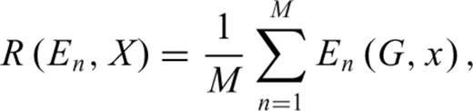
According to Rallo et al. (2002), one of the elements necessary for accurate SOM estimation is model diversity. Model diversity reflects the incorporation of training information characterizing variable relations across different spatial and temporal gradients. We visually explore the presence of model diversity in the underlying multivariate density function using component planes (Vesanto 1999). This representation provides information on the distributions of variables over the whole map (Vesanto 1999), and therefore reveals which map areas a certain attribute has the greatest influence. Visualization of correlated variables is possible by viewing several component planes.

A plot of the component planes (one component plane for each variable used in the training set; for example, UXO characteristics and ALLTEM measurements) for the APG calibration grid is presented in Fig. 5. The colour bar indicates the relative magnitude with largest in red colour and smallest values in the dark blue colour. Those component planes characterized by similar colour patterns have a high positive correlation, whereas similar patterns of opposite colour indicate a high negative correlation. For example, component planes of the time-based EMI amplitudes (volts), such as T0, T7, T22, T31, T45, are strongly correlated (ρ > 0.95) with each other and other gradient variables (volts μs^–1), such as 31M45, 31M60, 31M75, 31M105, 31M185, 31M250, 31M350, 31M450, 31M513. These component planes also depict a strong inverse correlation (ρ > −0.95) with other gradient variables, such as T105, T135, T185, T250, T350, T450, T513, T535. The amplitude at zero time (T0) is strongly correlated (0.97) with the amplitude at 7μs (T7) but drops off in time to a weak correlation (0.30) at T45 switching to a weak negative correlation (−0.14) at T60 which grows stronger until an almost perfectly negative correlation at T535 (ρ=−0.97). This amplitude also is strongly correlated (ρ > 0.97) with all of the gradient values except at 31M535 (ρ= 0.16).

Figure 5

SOM component planes (weights) of training data (32 731 records) collected over calibration grid at Aberdeen Proving grounds, Aberdeen, Maryland. There is one component plane for each variable used in the training set. Colour gradation from warm to cool characterizes high to low component values. Same colours (red or blue) at same locations implies positive relation, whereas opposite colours at same location implies negative relation.

Open in new tabDownload slide

In some cases, correlations are less obvious being restricted to similarities in colour at one or a limited number of component plane locations, such as the middle regions of inclination (inclin) and azimuth (azim) planes (Fig. 5). Temporal relations in the EMI signal amplitude also can be identified by noted changes in colours at a certain locations with time. For example, consider the red region at the lower left side of the early amplitudes (T0, T7, T22, T31, T45). In time, these amplitudes begin to reverse (T60, T75) becoming negative in their relation from that point to the last sample (T105, T135, T185, T250, T350, T450, T513, T535). A similar but less prominent reversal occurs at the lower right edge of these component planes. Still other component planes such those associated with EMI amplitude characteristics (alpha and tau) and subsurface target (item) characteristics (azimuth, depth, inclination) are more difficult to evaluate by a simple visual comparison because of the heterogeneity in structure. These relations are better evaluated using non-parametric statistics among pairs of component planes.

We present a summary of non-parametric statistics among component planes, namely p values and Spearman's rho values (Table 3). Inspection of this table reveals that the identify of subsurface targets (item) is independent of inclination (inclin), azimuth (azim) and tau; weakly related to alpha and depth, and strongly related to weight. These relations reveal attributes of target placement within the calibration grid and range of conditions under which SOM performance may be optimal. The correlations among target characteristics to those of the EMI measurements also are important, because it is this information content that can be used to assist in the target discrimination process. In general, these relations among target characteristics and EMI measurements are statistically significant with weak positive or negative correlations.

Table 3

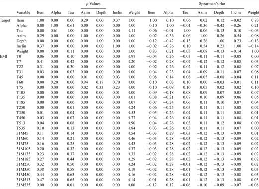
Statistical significance among component plane variables.

Open in new tabDownload slide

Using the remaining 50per cent (group 2) of the ALLTEM calibration data set (32 728 records), the trained SOM was then used to estimate target and associated characteristics as an independent performance test. A statistical summary of known and SOM estimated results is presented together in Table 4. False positives and false negatives are characterized as variation mostly outside the 25th and 75th percentiles. The median appears to be a robust estimator for azimuth (azim), depth (depth), inclination (inclin), target (item), weight (weight). For that reason, a summary of known and SOM-estimated median results for individual target patches (N indicates the number of records) are presented in Table 5. Inspection of this table reveals exceptional accuracy when estimating target type and its associated characteristics.

Table 4

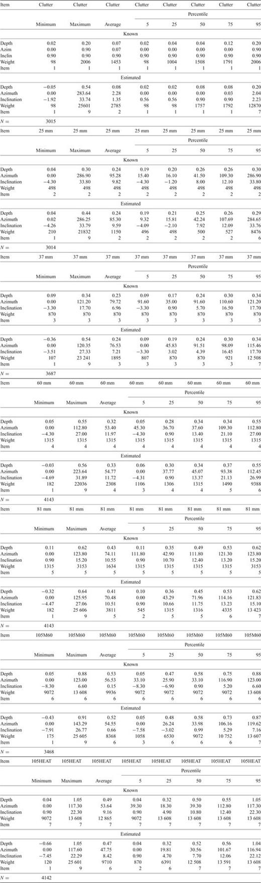
Summary of known and estimated characteristics for selected targets (all patches) using the trained self-organizing map.

Open in new tabDownload slide

Table 5

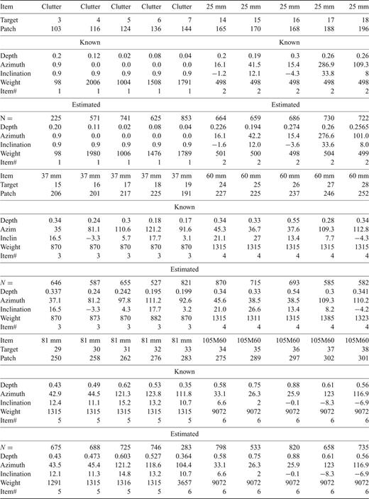
Summary of known and estimated median characteristics for selected targets (selected patches) using the trained self-organizing map.

Open in new tabDownload slide

A reasonable classifier is one without bias and yields strong correlation among data and estimated target parameter values, but such performance is ensured under only one set of conditions. For this reason, a subsequent examination of the SOM as a robust classifier is achieved by applying it to ALLTEM data collected over a blind grid.

4.2 Numerical discrimination for the APG calibration grid

The numerical inversion analysis results for the calibration grid at APG are presented as a scatter plot of inferred target lengths versus radii in Fig. 6. Classification of the known buried targets in the APG calibration grid using the algorithm outlined above resulted in a correct classification rate of 95per cent. This means that 76 of the 80 targets seeded in the grid were correctly identified as being of a certain kind of ordnance type. Three out of the four that were incorrectly classified were clutter which can have any shape, mass or other physical characteristics including resembling the types of ordnance that could be targets of interest. These types of missed classifications are called false positives. The fourth misclassified target was a false negative, declared as clutter when it should have been identified as a 105M60, one of the larger artillery types of ordnance. Upon closer examination, the calculated length and radii of the object were reasonable but the time-decay constant, tau, for this item was too low false negatives are more dangerous than false positives.

Figure 6

APG calibration grid numerical classification analysis results.

Open in new tabDownload slide

4.3 Hybrid classification

Classification of MEC using information from both the data-driven SOM and numerical classification constitutes a type of hybrid classification technique. The results from both the data-driven and numerical analyses are examined independently, then compared based on the level of confidence in each result for a given target. The level of confidence considered for the data-driven analysis is measured by the degree of scatter of the results. That is, do the majority of the results indicate one type of target or do they indicate a whole range of items from small to large munitions with no inference on which is the best result. The level of confidence for the numerical analysis is measured by the mean-square error (MSE) of model to data misfit. The refinement of the data provided to each analysis is based on the confidence in each result. Hence, this may be called a cooperative classification result.

For example, the first run of a hybrid classification from the Blind Test grid is presented in Fig. 7. In this figure are shown both the Calibration and Blind Test grid results. Scoring of these results was as follows: Of the UXO detected, theper cent called UXO was 95per cent and of the clutter detected, theper cent called UXO was 55per cent. Problems were noted generally with the larger items (81 and 105 mm projectiles). Note the large amount of scattering of the Blind Test grid results in Fig. 7 about the known targets from the calibration grid. For example, the objects classified as being 25 mm projectiles have lengths 0.049–0.075m and radii 0.010–0.023m for the known calibration targets but have lengths 0.021–0.08m and radii 0.006–0.030m for the Blind Test grid data. The relatively poor performance led to a re-examination of the SOM analysis for each target in the Blind Test grid.

Figure 7

APG Blind Test grid hybrid classification analysis results, Run 1. Scoring was as follows: of UXO detected,per cent called UXO – 95per cent; of clutter detected,per cent called UXO–55per cent, problems generally with larger items (81 and 105 mm).

Open in new tabDownload slide

The detailed re-examination of the SOM results revealed some issues that need to be resolved. If the SOM analysis results in a cluster around an item that is not part of the training item set, the SOM will indicate that item in the training set that is closest in character (size, shape). This resulted in many clutter items being classified as UXO (55per cent) because an insufficient number of clutter items were present in the training set. Another example is presented in Fig. 8. The SOM result indicates a 25 mm projectile. However, the numerical inversion results (length 0.045m and radius 0.024 m) indicate that this item is a small clutter item. Because the SOM did not have a similar training item, it chose the smallest ordnance item from the training set.

Figure 8

SOM issue #∼1—plot of SOM result and table of numerical inversion result. SOM analysis indicates ordnance whereas numerical analysis indicates clutter. This is a result of SOM fitting unknown data to the only training data it is provided.

Open in new tabDownload slide

A second issue is that the SOM often cannot decide between multiple items with very different characteristics. An illustration is presented in Fig. 9. The SOM analysis indicates that this item could either be a piece of clutter (item #1), a 37 mm projectile (item #3) or a 60 mm projectile (item #4). The numerical inversion results, however, indicate with high confidence that the item is a 37-mm projectile. A third issue is that the SOM can indicate two items with similar shape but of different sizes. This occurred several times with 37 and 105 mm projectiles and with 25 and 81 mm projectiles. Illustrations of these occurrences are presented in Figs 10 (37s and 105s) and 11 (25s and 81s) including images of the specific ordnance items.

Figure 9

SOM issue #2—plot of SOM results and table of numerical inversion results. SOM indicates multiple MEC-type items whereas numerical classification indicates 37-mm ordnance with high confidence (low mean-square error).

Open in new tabDownload slide

Figure 10

SOM issue #3—plot of SOM results and table of numerical inversion results. SOM indicates two items based on a shape factor; that is, the SOM indicated two items that have the same shape with the exception that one is much smaller than the other. A 37-mm diameter projectile is shown below left and a 105-mm diameter projectile is shown below right.

Open in new tabDownload slide

Figure 11

SOM issue #3 – Plot of SOM result and table of numerical inversion result. SOM indicates two items based on a shape factor; that is, the SOM indicated two items that have similar shape with the exception that one is much smaller than the other. 25-mm and 81-mm diameter projectiles are shown below the plot.

Open in new tabDownload slide

Resolution of the first issue is achieved by including more ordnance and more clutter items in the training data. A more diverse training set could create more ambiguities but also allows more flexibility in identifying various targets. The second issue is likely because of noise being provided as input to the SOM. To reduce the noise, the low-amplitude data on the edges of the anomaly should be removed and only the high quality signal be included. This is accomplished by reducing the size (area) of the anomaly data patches.

The anomalous data patches from the orthogonal data recorded with the Hx and Hy transmitters are smaller than those from the Hz transmitter because less signal penetrates the ground. Fig. 12 presents significant data (data with signal amplitudes above the background) from both vertical and horizontal receiver components. The horizontal component data have smaller footprints than the vertical components. This implies that non-contributing noise preferentially contaminates the horizontal component data. The first nine receiver polarities include many horizontal components that provide critical information about the orientation (azimuth and inclination) of the buried targets. Receiver polarities based on signal strength are selected after the ninth polarity. Currently, 14 of the 19 available receiver polarities are utilized by the numerical inversion.

Figure 12

Examples of ALLTEM data for receiver polarities ZZM and ZZH (vertical transmitter) and XZH and YZH (horizontal transmitters). Note the differences in the sizes of the anomalous areas of the significant data for the same target for these types of receiver components. The patch data for the XZH and YZH components are somewhat smaller than the ZZH component and distinctly smaller than the ZZM component data.

Open in new tabDownload slide

The considerations just described support reduction of the size of the anomaly patches, and thus the noise, used for both the numerical inversion and SOM analysis. An example of patch-size reduction is presented in Fig. 13. The left hand side of Fig. 13 shows the original data patches (Run 1) whereas the right-hand side shows the reduced patches (Run 2). SOM results from both Run 1 and Run 2 for patch 152 from the Blind Test grid are presented in Fig. 14. The left-hand side shows the results for Run 1. Note the same ambiguity in target identification. The right side shows the results from Run 2. The target detected in patch 152 is a 105M60 projectile.

Figure 13

Illustration of reduction in patch size resulting in reduction of data containing noise from Run 1 to Run 2.

Open in new tabDownload slide

Figure 14

Example of change in anomalous data patch size area on SOM analysis results from Run 1 to Run 2. These data also present another illustration of issue #3.

Open in new tabDownload slide

The full hybrid classification results using both the SOM and numerical inversion and classification are presented in Fig. 15. There is less scatter than before. Of the UXO detected, theper cent called UXO was 95per cent and of the clutter detected, theper cent called UXO was only 25per cent. More research on refining the SOM and numerical classification protocols is required. This might include being more discerning about which data from the nineteen receiver polarities are provided to the SOM and numerical inversion and also how many data points of those provided are actually required to produce a quality result. Another example is that only the large 1-m-loop receivers (ZZM, XZM and YZM) are useful for the deeper targets. The small horizontal receiver components are insensitive to secondary signals from the deeper targets and contribute only noise to the data set.

Figure 15

APG Blind Test grid hybrid classification analysis results, Run 2. Scoring: 100per cent UXO detected,per cent called UXO–95per cent; of clutter detected,per cent called UXO–25per cent.

Open in new tabDownload slide

5 Conclusions

A hybrid processing approach has been successfully applied to ALLTEM data for accurate field classification and discrimination of overlapping UXO from clutter in the presence of geological noise. We find that the SOM can be trained on one data set and then used with other data sets to classify multiple target types and estimate their characteristics. False positives and false negatives are minimized using the median estimate of target characteristics recorded using multiple records over a field target. Limitations of this hybrid classification protocol have been identified and research focuses on refining what data are used, how the data are used and what the results actually communicate. Overall, the ALLTEM system shows promise as a rapid, reliable, and cost-effective method for cleanup of UXO-contaminated lands.

Acknowledgments

We are grateful to Robert Horton of the USGS and the anonymous reviewers for their critical reading of the manuscript and suggestions. This work was financially supported by the U.S. Department of Defense Environmental Security Technology Certification Program (ESTCP) under project number MM-0809.

References