GOCE satellite derived gravity and gravity gradient corrected for topographic effect in the South Central Andes region

Summary

1 Introduction

The Andes are constructed from a complex puzzle of lithospheric blocks that have been amalgamated since the formation of the Rodinia supercontinent, up to 5 Ma (see Ramos 2009). Some pieces were attached as the consequence of important collisions that have produced and exhumed metamorphic belts and obducted long strips of oceanic lithosphere. Other blocks are associated with the closure of small backarc basins or the collision of different kinds of oceanic crust terranes. The record of these amalgamations is highly variable in quality due to the subsequent orogenic processes that affected, firstly the western border of Gondwana, and then the South American plate since the opening of the Atlantic Ocean (Somoza & Zaffarana 2008). The Andes, and the associated subduction processes, are the product of the westward shift of the South American plate since the fragmentation of Pangea. These processes altered and obscured the basement geometry, displacing previous anisotropies, developing foreland basins and buried the basement beneath thick columns of arc and retro-arc volcanic material (Tunik et al. 2010).

In particular, the Pampean flat slab zone developed between 27°S and 33°S, exhibits an intricate collage of crustal blocks that amalgamated during the Pampean (Brasiliano), Famatinian and San Rafael (Alleghinian-like) deformational stages, that is far from being completely understood (see Ramos 2009 for references therein). Its timing and particularly its pattern are intensely discussed due to basin formation phenomena that have defined sparse basement outcrops. Despite this incomplete record, these amalgamations have defined important compositional and therefore density heterogeneities.

Mass inhomogeneities affect Earth's gravity field and its related properties. Satellite gravimetry is highly sensitive to variations in the gravity field; therefore, the gravity field and its derivatives can be determined using either orbit monitoring or acceleration and gradient measurements at satellite heights. Recent satellite missions, namely the Challenging Mini-satellite Payload (CHAMP), Gravity Recovery and Climate Experiment (GRACE) and now Gravity field and steady-state Ocean Circulation Explorer (GOCE) have resulted in extraordinary improvement in the mapping of the global gravity field. High-resolution gravity-field models based on observations of satellite data in addition to terrestrial data, and are available as spherical-harmonic coefficients, for example, EGM08 with maximum degree and order of N = 2159 (Pavlis et al. 2008). This allows for regional gravity modelling, and the studying of the crust and lower lithosphere at regional scale. For geoid determinations, topographic effect must be removed from the satellite observations (Forsberg & Tscherning 1997). The effect generated by topographic masses on the gravity field and its derivatives is calculated according to Newton's law of universal gravitation. To calculate the topographic effect, it is necessary to know the topography around each point. Therefore, topographic masses are subdivided into elementary bodies for which there is a closed solution of the mass integrals (Torge 2001). Molodensky (1945) demonstrated that the physical surface of the Earth can be determined based solely on geodetic measurements without using a predetermined hypothesis regarding the density distribution within the Earth. However, a mean density must be assumed in order to calculate the topographic contribution. Spherical prisms (i.e. tesseroids) of constant density are especially appropriate because they are easily obtained through simple transformations from digital elevation models (DEMs). Therefore, the effect of each mass component can be calculated separately, and all of the individual effects can be added to calculate the total effect (Heck & Seitz 2007; Grombein et al. 2010). Mapping was done from the topographical reduced fields implementing EGM08 and GOCE. Afterwards they were compared to a schematic geological map of the South Central Andes region, which includes the main geological features with regional dimensions and may reveal crustal density variations.

This work focuses on the determination of mass heterogeneities that are related to discontinuities in the pattern of terrain amalgamation that make up the basement over the Pampean flat slab zone.

2 Geological Setting

The study area straddles the Pampean flat subduction zone (dip angle of ∼5°), developed in the last 17 Ma, between two segments of normal subduction zones (dip angle of ∼30°) (Fig. 1; Jordan et al. 1983a; Ramos et al. 2002).

Figure 1

Terrain boundaries and main geological provinces of the study area.

Open in new tabDownload slide

This segment is associated with vast regions elevated above 4000 m, and a wide deformational zone that extends beyond 700 km east of the trench. Multiple authors (Allmendinger et al. 1997; Kay et al. 1999; Gutscher et al. 2000; Kay & Mpodozis 2002; Ramos et al. 2002) have linked the eastward expansion and subsequent extinction of the Miocene to Quaternary volcanic arc and contemporary migration of the compressive strain towards the foreland with the gradual flattening of the subducted slab.

The basement of the Pampean Ranges encompasses two magmatic belts with arc affinities. The eastern belt comprises a late Proterozoic–Early Cambrian age magmatic and metamorphic belt bounded by ophiolitic rocks known as the Pampean orogen, and is considered the result of the final amalgamation to the Río de la Plata craton (Kraemer et al. 1995; Rapela et al. 1998). Its western belt comprises an Ordovician magmatic and metamorphic suite known as the Famatinian orogen. This orogen and related arc rocks are explained as the result of the final amalgamation to the Laurentia derived Cuyania exotic block and collision with the para-auctocthonous Antofalla block (see Ramos 2009, for a review).

The Famatinian system is a set of basement blocks located west of the Western Sierras Pampeanas (Fig. 1). These systems share a common origin associated with the flat subduction processes that occurred in the area, being differentiated by their Palaeozoic cover and metamorphic grade (González Bonorino 1950). To the west, the Precordillera is a east-verging system with imbricated Late Proterozoic to Triassic sequences, whose basal terms have been interpreted as Laurentic derivation (Cuyania; Fig. 1) and accreted against the Gondwana margin in Late Ordovician times (see Ramos 2004, for a review). This deformation occurred in the last 10 Ma, synchronously with the compressive rise of the Pampean Ranges to the east (Jordan & Allmendinger 1986; Ramos et al. 2002).

Geophysical data (Snyder et al. 1990; Zapata 1998; Introcaso et al. 2004; Gilbert et al. 2006) show a sharp boundary between the two adjacent and contrasting crusts of Pampia and the Cuyania terrane. Recent aeromagnetic surveys (Chernicoff et al. 2009) have inferred a mafic and ultramafic belt interpreted as a buried ophiolitic suite hosted by its corresponding suture. This boundary coincides locally with basement exposures of high to medium grade metamorphic rocks developed in close association with the Famatinian orogen of Early to Middle Ordovician age (Coira et al. 1982; Rapela et al. 1998, 2001; Otamendi et al. 2008, 2009; Chernicoff et al. 2010). Lower crustal rocks are exposed along this first order crustal discontinuity, which is interpreted as, the suture between Pampia and the Cuyania terrane at these latitudes (Ramos 2004; Ramos et al. 2010). This discontinuity, known as the Valle-Fertil lineament and its continuation into the Desaguadero lineament is disposed in a NNW direction along 700 km. Gimenez et al. (2000) interpreted zones of high density buried materials from gravity datasets, along with this Valle Fertil lineament.

West of Cuyania, the Chilenia terrane is separated by a Late Ordovician age ophiolitic belt (Ramos et al. 1984). Its history remains somewhat obscure, U-Pb ages and Nd model ages point to Laurentian origin for its basement as well. The lack of palaeomagnetic data precludes determining its kinematic evolution. However, it is considered to have been separated from the Gondwanian continent to which it eventually accreted at ∼420–390 Ma. Its basement is mainly exposed at the Frontal Cordillera, that is formed by a series of Neo-proterozoic to Palaeozoic basement blocks, that stand west of the Precordillera and constitutes the highest elevation of the fold and thrust belt at these latitudes. To the west a Mesozoic basin is incorporated into the Main Andes by contraction, characterized by a mixed deformational style that varies from thin to thick-skinned mechanics (Ramos et al. 2002).

The Chacoparanense plain is developed over the Río de la Plata region that bounds to the west with the Pampean Ranges uplifted in the last 10 Ma and detached from Proterozoic to Triassic discontinuities that affected the Pampian basement (González Bonorino 1950; Caminos 1979; Casquet et al. 2008; Ramos et al. 2010; Allmendinger et al. 1983; Jordan et al. 1983a,b). The Chacoparanaense plain was first characterized by Groeber (1938) as a vast plain developed between the Sub-Andean ranges and the Pampean ranges to the west and the Parana River to the east. Its most conspicuous feature is the extensive development of a wide marine transgression of mid-Miocene age derived from the Atlantic ocean in the east (13–15 Ma), that almost covered the plain completely (Ramos 1999). Even though its deposits do not outcrop, they have been mostly detected through boreholes practically throughout its full extension (Groeber 1929; Windhausen 1931; Rapela et al. 2007, 2011).

The Río de la Plata basement outcrops, extend from southern Uruguay to central-eastern Argentina with a surface of approximately 20000 km². The Rio de la Plata craton is covered by a thick pile of younger sediments, from which its true extent is only inferred indirectly (Rapela et al. 2011). The oldest rocks there have been dated as being 2200 and 1700 Myr of age, indicating that they constituted a different block other than Pampia. Metamorphic and magmatic belts located east, indicate that it had already been attached to African-Gondwanian blocks by the late Proterozoic. The boundary between Pampia and the Rio de la Plata craton is not exposed (Ramos et al. 2010). However, a strong gravimetric anomaly identified in the central part of the Sierras de Córdoba foothills by Miranda & Introcaso (1996) indicates a first order crustal discontinuity that has been related to their collision in Neoproterozoic times (Ramos 1988; Escayola et al. 2007). The crustal discontinuity of the eastern margin of the Sierras de Córdoba has been correlated with a continental scale lineament, the Transbrasiliano lineament, which is a continental scale structure (López de Luchi et al. 2005; Rapela et al. 2007; Favetto et al. 2008; Ramos et al. 2010).

3 Gravity Derivatives for Identifying Main Geological Structures

The most recent satellite mission GOCE has gained extraordinary improvement in the global mapping of the gravity field, through the orbit monitoring, acceleration and gradient measurements taken at satellite heights. However, GOCE data is not yet integrated with terrestrial data within a global gravity field model. The last high resolution gravity field model EGM08 (Pavlis et al. 2008), is a combined solution composed of a worldwide surface (land, marine and airborne) gravity anomaly database with a 5′× 5′ resolution, and GRACE derived satellite solutions, that takes advantage of all the latest data and modelling for both worldwide land and marine areas, and is presented as sets of coefficients of a spherical harmonic expansion of the gravity field. In the case of EGM08, maximum degree and order are N = 2159, with some additional terms up to degree/order 2190 (Pavlis et al. 2008). The spatial resolution of the model depends on the maximum degree N_max (Barthelmes 2009), so the relation between spherical harmonic degree N and the smallest representative feature of the gravity field resolvable with EGM08 potential field model is equal to λ_min≈ 2πR/N_max≈ 19 km with R being the mean Earth radius and N_max the maximum degree and order of the harmonic expansion (Li 2001; Hofmann-Wellenhof & Moritz 2006; Barthelmes 2009). The observed potential is obtained from the global gravity field model. Then, the disturbing potential (T) is obtained (Janak & Sprlak 2006) by subtracting the potential field of the reference ellipsoid from the observed potential. The gravity anomaly is obtained as the first spatial derivative of T and a correction term, and the gravity gradient tensor (Marussi tensor) is composed by five independent elements and is obtained as the second derivatives of the disturbing potential (e.g. Hofmann-Wellenhof & Moritz 2006).

3.1 GOCE versus EGM08 data comparison

The preliminary model derived from data of the GOCE mission is now available however, with a lower spatial resolution (N = 250, Pail et al. 2011) than mixed satellite-terrestrial global models like EGM08 (Pavlis et al. 2008). Nevertheless it is useful to examine the quality of the terrestrial data entering the EGM08 by a comparison analysis with the satellite-only gravitational model of GOCE (Pail et al. 2011). For degrees greater than N = 120, EGM08 relies entirely on terrestrial data. A simple way to evaluate the quality of the terrestrial data contributing to the model is to make a comparison analysis up to degree N = 250 with the pure GOCE-satellite derived model. In a recent paper (Braitenberg et al. 2011b), showed in detail how errors at high degree, enter the error of a downscaled EGM08: in short, if the complete EGM08 up to N = 2159 locally (that is at wavelengths smaller than, e.g. 400 km) is considered to be derived from the gridded terrestrial measurements with nominal resolution of 9 km, then a downscaling of the field to an 80 km resolution can be made, by averaging the observations. It is clear then, that the downscaled data are severely affected by the errors of the original data. In fact, by the propagation law of errors, the expected uncertainty on the averaged value may be calculated, given the starting errors. Assuming that the errors of the GOCE data are homogeneous in space, variations in the standard deviations of the EGM08/GOCE differences are attributed only to the initial errors of the terrestrial data. If GOCE data, available to degree and order N = 250, is compared with the EGM08 data at the same degree, it is known that the degrees between 70 and 120 of the EGM08 model are based increasingly on terrestrial data, and between 120 and 250 entirely on terrestrial data. According to the aforementioned considerations, therefore the errors of the original terrestrial data are heavily affecting the errors of the EGM08 values up to N = 250, because the spherical harmonic expansion can be seen as an averaging process. The standard deviations between GOCE and EGM08 thus represent varying quality of the original terrestrial data, because the quality of the GOCE data is locally homogeneous. Where the standard deviations are small, the original data must have been accurate or otherwise the same downscaled values and a small standard deviation would only have been obtained by chance. Therefore, GOCE is a remarkably important independent quality assessment tool for EGM08. By comparison of the gravity anomaly (Fig. 2a) derived from the EGM08 model (Pavlis et al. 2008) and at the same time derived from the GOCE satellite (Pail et al. 2011; Fig. 2b), it can be shown that the fields are only in partial agreement, and the differences are smooth. The absolute value of the difference field (EGM08-GOCE) is shown in Fig. 3.

Figure 2

Quality control of the EGM08 gravity model, which combines terrestrial and satellite data, with GOCE satellite-only-derived gravity model. Maximun degree and order N = 250. (a) Gravity anomaly obtained with EGM08. (b) Gravity anomaly obtained with GOCE. National borders: dashed lines; province borders: thin black lines; coastal borders: black lines.

Open in new tabDownload slide

Figure 3

Absolute difference between the two fields. The black square shows the area (over the Andes) with erroneous data. The white square shows the area (over the plain) with good data. National borders: dashed lines; province borders: thin black lines; coastal borders: black lines. The differences between the two fields are due to erroneous terrestrial data or lack of it in the EGM08 model.

Open in new tabDownload slide

Statistical parameters for the difference between the two fields are: average difference = 0.077 mGal, standard deviation = 12.34 mGal, maximal value of difference = 62.021 mGal. A high-quality region is compared with a low-quality region in terms of the residual histogram. The black square in Fig. 3 marks a 2°× 2° area with degraded quality; which is compared to a square of equal size (white) of relatively high quality. The histograms of the residuals (Fig. 4) illustrate the higher values for the black square (over the Andes region). The rms deviation was calculated from the mean on sliding windows of 1°× 1° as a statistical measure of EGM08 quality. The result is shown on Fig. 5. The most frequent value of the rms deviation is 6 mGal as is shown in Fig. 6. The locations where the terrestrial data have problems reflected greatly increased values (up to 23 mGal).

Figure 4

Histogram of the residual gravity anomaly between EGM08 and GOCE (up to degree and order N = 250). Left (Bad tile): black square of Fig. 3. Right (Good tile): white square of Fig. 3.

Open in new tabDownload slide

Figure 5

Root mean square of the gravity residual on 1°× 1° tiles.

Open in new tabDownload slide

Figure 6

Histogram of the rms deviations on 1°× 1° tiles.

Open in new tabDownload slide

Differences are due to the sparseness of the terrestrial data in large regions, especially in those of difficult access, and to a non-unified height system used in different terrestrial campaigns. The accuracy of the (in-land) gravity observations and their derivatives depends on the precision of the height measurements, where greater inconsistencies arise when considering large areas (Reguzzoni & Sampietro 2010). This highlights the usefulness of satellite derived data in mountainous areas of difficult access, as is the western zone of the region under study. Furthermore the global gravity fields are useful to merge the terrestrial data by means of controlling the longer wavelengths. Nevertheless, the shorter wavelengths are still best defined by the terrestrial data.

3.2 The topography-reduced gravity anomaly

The generalized gravity anomaly Δ_g according to Molodensky′s theory (Molodensky et al. 1962; Hofmann-Wellenhof & Moritz 2006), explained by Barthelmes (2009), is the magnitude of the gravity, g, at a given point (h, λ, φ) minus the normal gravity, γ, at the same longitude and latitude, but at the ellipsoidal height h –ζ_g, where ζ_g is the generalized height anomaly

1

The height h is assumed on or outside the Earth's surface, that is, h ≥ h_t, hence the gravity anomaly is a function in the space outside the masses. Thus, the measured gravity at the Earth's surface can be used without downward continuation or any reduction (Barthelmes 2009).

The topography-reduced gravity anomaly, explained by Barthelmes (2009), is the difference between the real gravity and the gravity of the reference potential and which, at the same time, does not contain the effect of the topographical masses above the geoid. By using a digital terrain model of the entire Earth and, a mass density distribution hypothesis, the potential V_t can be calculated approximately (Barthelmes 2009). Such anomalies are useful for highlighting the effects of different rock densities of the crust. Thus, the topography reduced gravity anomaly is (see Barthelmes 2009 for a review):

2

where W is the real potential at a given point (h, λ, φ), V_t is the gravity potential of the topography at the same point and U is the gravity of the reference potential at the same longitude and latitude but at the h –ζ_g height.

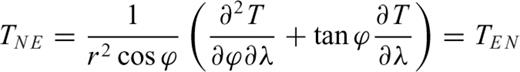
3.3 The Marussi tensor

The Marussi tensor (M) is composed of five independent elements and is obtained as the second derivative of the disturbing potential (Hofmann-Wellenhof & Moritz 2006; Rummel et al. 2011):

3

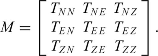
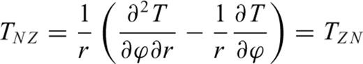
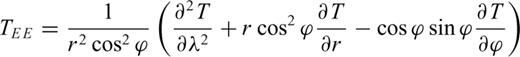
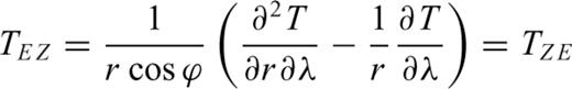
In the spherical coordinate system, the Marussi tensor components are given by Tscherning (1976). Where T[r, ϕ, λ] is the disturbing potential, r the radial distance and ϕ, λ the latitude and the longitude, respectively:

3a

3b

3c

3d

3e

3f

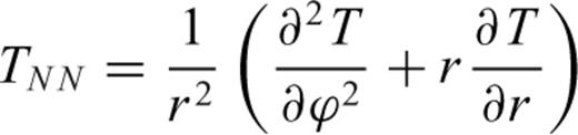
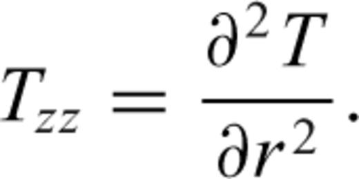
Braitenberg et al. (2011a) mapped the gravity anomaly and the vertical gravity gradient (T_zz) generated by a spherical prism in order to determine which of the two best enhances the anomalous mass. They explained that T_zz is centred on mass, giving a positive signal over the body, and a small amplitude negative stripe along the borders. On the other hand, the gravity anomaly does not show the negative stripe pattern along the borders and the anomaly pattern is broader. Therefore, for geological mapping the T_zz component is ideal, as it highlights the anomalous mass centre with higher resolution than gravity as exposed by Braitenberg et al. (2011a). This allows authors to unravel unknown geological structures that are either concealed by sediments or have not been mapped yet.

4 Gravity Gradients for Tesseroids

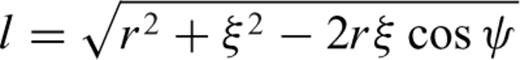
A tesseroid is an elementary body bounded by geographical grid lines on an ellipsoidal (or spherical) reference surface or surfaces of constant ellipsoidal (or spherical) height (Anderson 1976; Heck & Seitz 2007). The bounding surfaces of a tesseroid (Fig. 7) consist of a pair of constant ellipsoidal height surfaces (h₁ = const, h₂ = const), a pair of meridional planes (λ₁ = const, λ₂ = const), and a pair of coaxial circular cones (ϕ₁ = const, ϕ₂ = const). In most cases, a spherical approximation of the ellipsoidal tesseroid will yield sufficient results (Novák & Grafarend 2005; Heck & Seitz 2007). By neglecting the elliptic features of the reference surface, the pair of constant ellipsoidal height surfaces (h₁, h₂) then consists of concentric spheres with radii r₁ = R + h₁ and r₂ = R + h₂, where R denotes the chosen radius of the equivalent sphere.

Figure 7

Tesseroid geometry in a global coordinate system (Kuhn 2000).

Open in new tabDownload slide

The potential of the masses can be described by the Newton integral in spherical coordinates (Heiskanen & Moritz 1967; Blakely 1995)

4

4a

4b

where (r, ϕ, λ) are spherical coordinates of the point of calculation P (ξ, ϕ', λ') are spherical coordinates of the integration point Q of the variable related to a terrestrial reference frame, l is the Euclidean distance between two points and ψ is the angle between the position of vectors P and Q. 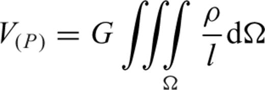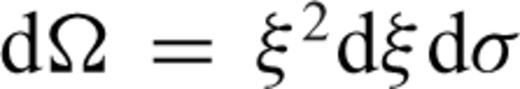The universal gravitational constant is G = 6.673 × 10⁻¹¹ m³ kg^–2 (Wild-Pfeiffer 2008), ρ is the local mass density and is the volume element. To make topographic masses discrete, segmentation should be performed in the volume elements Ω_i, where the density ρ_i is assumed to be constant. Then, the potential of a tesseroid is

5

This triple integral of the gravitational potential and its first and second derivatives, do not have analytical solutions. To solve the triple integral, purely numerical methods must be applied using one of three methods: an integral kernel expansion of a Taylor series, the method of Gauss–Legendre quadrature (GLQ) 3-D, or by splitting the integral into a one-dimensional integral over radial parameter ξ, for which there is an analytical solution, and a spherical 2-D integral, which is determined using a GLQ method (Asgharzadeh et al. 2007; Wild-Pfeiffer 2008; Grombein et al. 2010).

4.1 TGG for a synthetic topography

The software Tesseroids (Uieda et al. 2010) performs direct calculation of the gravity gradient tensor components using the GLQ. The geometric element used in the modelling processes is a spherical prism (tesseroid) (Anderson 1976; Heck & Seitz 2007; Wild-Pfeiffer 2008). This new software is of special interest for the study of large areas, where the flat Earth approximation can have its limitations. In these cases the modelling could be done with tesseroids, in order to contemplate the Earth's curvature (Uieda et al. 2010). A synthetic topography of 10°× 10° with a central prism of constant height and 1' grid spacing was generated. The prism dimensions were 1°× 1° with 1 km of height centred at latitude 50°N and longitude 0°. The obtained TGG components are shown in Fig. 8. A height of 250 km was used for point Q to determine the effect on the orbit of the GOCE satellite. To examine the differences between the calculation with spherical prisms and with rectangular ones, the same calculation was performed using the TC software (Forsberg 1984). This software performs calculations using rectangular prisms (Nagy 1966; Nagy et al. 2000). Statistical parameters for the difference between both T_zz components are: maximum difference = 0.0161 Eötvos average difference = 0.00172 Eötvös, standard deviation = 0.00327 Eötvös.

Figure 8

TGG generated using a tesseroid of 1°× 1°× 1 km, and a height calculation of 250 km, calculated with Tesseroids software (Uieda et al. 2010).

Open in new tabDownload slide

The same calculation was made at lower heights in order to analyse the difference between the two methods in more detail (Fig. 9). The calculation height of 7000 m was selected since it is the same one used for the topographic effect calculation. Statistical parameters for the difference between both T_zz components are: maximum difference = 24.633 Eötvos, average difference = 0.003495 Eötvos, standard deviation = 0.9096 Eötvos. The difference between each corresponding component of the TGG obtained by the calculation with both methods at 7000 m is shown in Fig. 10. Calculation with spherical prisms shows a slightly higher effect inside the body that decreases towards the centre. The difference is greater towards the edges and in the corners, this effect being greater when calculated with rectangular prisms. Outside of the body, the effect calculated with spherical prisms is lower when compared to that calculated with rectangular ones.

Figure 9

TGG generated using a tesseroid of 1°× 1°× 1 km, and a height calculation of 7000 m, calculated with Tesseroids software (Uieda et al. 2010).

Open in new tabDownload slide

Figure 10

Difference between TGG components obtained by calculation with rectangular prisms method (Forsberg 1984) minus spherical prisms method (Uieda et al. 2010).

Open in new tabDownload slide

From the comparison of the results a great consistency between the two methods and a slight improvement in resolution for calculations with spherical prisms can be inferred; that is, calculating with rectangular prisms improperly magnifies the effect over the edges.

4.2 Topographic correction calculation

The topographic effect is removed from the fields to eliminate correlation with the topography. The DEM expressed in a geodetic coordinate system (λ₁, ϕ_1,h) is converted into a set of tesseroids (mass elements) of constant density that are expressed in a geocentric coordinate system for calculation. The calculation of the topographic effect for the GA and T_zz (Fig. 11) is performed using the Tesseroids software (Uieda et al. 2010) at 7000 m calculation height, on a regular grid of 0.05° grid cell size. The region between latitudes 25°S and 35°S and longitudes 75°W and 60°W was selected for the calculation. The DEM used is ETOPO1 (Amante & Eakins 2008), a 1 arcmin cell spacing global relief model of Earth's surface that integrates land topography and ocean bathymetry.

Figure 11

Topographic correction obtained from a DEM (ETOPO1). (a) Topographic correction for gravity anomaly. (b) Topographic correction for T_zz.

Open in new tabDownload slide

The correction amounts up to tens of Eötvös for the vertical gradient and up to a few hundreds of mGal for gravity. It is greatest over the highest topographic elevations (e.g. the Puna and the Andes Cordillera) and over the lower topographic depressions as in the Chilean trench.

5 The Gravity Derived Quantities and Their Relation to Geology

Using the global model EGM08 (Pavlis et al. 2008), the vertical gravity gradient and the gravity anomaly for South Central Andes are calculated (Janak & Sprlak 2006) on a regular grid of 0.05° grid cell size, with a maximum degree and order equal to 2159 of the harmonic expansion. The calculation height is 7000 m to ensure that all values are above the topography and is made in a spherical coordinate system. All calculations are carried out with respect to the system WGS84. A standard density of 2.67 g cm⁻³ for continental crust and a density of 1.03 g cm⁻³ for the sea were used. Topography corrected gravity anomaly is shown in Fig. 12 and topography corrected vertical gravity gradient is shown in Fig. 13. Comparison of the gravity and the gradient field reveals an optimal correlation in the location of the anomalies, the T_zz resolving in a more accurate way.

Figure 12

Gravity Map anomaly corrected by topography for EGM08 model up to degree and order N = 2159. Lineaments: C, Catamarca; S, Salado; T, Tucuman; TB, Transbrasiliano; VF, Valle Fértil Desaguadero. Terranes: AA, Arequipa Antofalla; F, Famatina; PC, Precordillera. Basins: B, Bermejo; CU, Cuyana; P, Pipanaco; R, Valle de la Rioja; SG, Salinas Grandes. Minor saws: A, Ancasti; CB, Cordoba. MT profile is from Favetto et al. (2008), boreholes are from Rapela et al. (2007). Terrain boundaries depicted as dashed line; Great lineaments depicted as dotted line; Precordillera: dot and dashed line; Chile trench: continuous line.

Open in new tabDownload slide

Figure 13

Map of the vertical gravity gradient corrected by topography for model EGM08, and up to degree and order 2159. Lineaments: C, Catamarca; S, Salado; T, Tucuman; TB, Transbrasiliano; VF, Valle Fértil Desaguadero. Terranes: AA, Arequipa Antofalla; F, Famatina; PC, Precordillera. Basins: B, Bermejo; CU, Cuyana; P, Pipanaco; R, Valle de la Rioja; SG, Salinas Grandes. Minor saws: A, Ancasti; CB, Cordoba. Terrain boundaries depicted as a dashed line; great lineaments depicted as dotted line; Precordillera: dot and dashed line; Chile trench: continuous line. Rio de la Plata craton boundary: double dot and dashed line (as is not clearly detected in T_zz).

Open in new tabDownload slide

Results obtained are compared to a schematic geological map of the South Central Andes region, which includes the main regional dimension geological features, which presumably are accompanied with crustal density variations. The main lineaments, intrusions, and foreland basins have been interpreted, mostly corresponding to Pampean Ranges which are located in the central strip of the map.

The contact area between the Cuyania and the Pampia terranes, associated with the Valle Fertil–Desaguadero megalineament (Gimenez et al. 2000; Introcaso et al. 2004), is detected in the GA signal (Fig. 12) and is also revealed in the gravimetric gradient due to the abrupt negative to positive change (Fig. 13). To the west of the central part of this contact area, the Bermejo basin is depicted, which presents gradient values between −13 and −45 Eötvös and up to −300 mGal for gravity. South of this basin the Pie de Palo mountain range is located, an exposure of Mesoproterozoic crystalline basement, which is identified by its high gravimetric signal reaching +190 mGal, and +72 Eötvös for T_zz. To the east of the Bermejo basin, the Ordovician plutonic rocks of the Valle Fertil mountains are located, and are limited to +160 mGal for GA and exceeding +52 Eötvös for T_zz. These mountains form part of the Famatinian arc within the Pampean Ranges. Relative positive values are due to a negative regional trend provoked by the Andean root. T_zz shows a positive signal which fluctuates to negative values due to intermountain basins.

Within the western part of the Cuyania terrain (Fig. 12), the positive gravimetric response of the Precordilleran influence on the great negative influence of the Andean root can be clearly seen. The Ordovician-Devonian and the Cambrian-Ordovician sedimentary rocks that conform the Precordillera present GA values between −90 and −4 mGal, and +60 Eötvos for T_zz. The western limit of the Precordillera is marked by a NS semi-arched elongated anomaly, presented as a minimum of both gravity (reaching −391 mGal) and the vertical gravity gradient (up to −97 Eötvös), which marks the boundary between the Cuyania and the Chilenia terrain. The Cuyana Basin is located South of the Precordillera.

Within Pampia, foreland basins as Pipanaco (Dávila et al. 2012), Valle de la Rioja (Gimenez et al. 2009), and Salinas Grandes present low gradient values between −30 and +6 Eötvös for T_zz and are limited to −170 mGal for gravity. Pampean ranges as Chepes, Velasco, Ambato and Capillitas, composed by Ordovician plutonic rocks present a notorious signal in gravity and in T_zz. Ancasti is composed by medium to high grade Neoproterozoic-Cambrian meta-sedimentaty present a broader pattern.

On the eastern margin of the Pampean Ranges, the contact area between the Pampia terrane and the Río de La Plata craton, the Tranbrasiliano lineament, can be clearly observed in the gravity anomaly (Fig. 12), expressed by an abrupt change of the gravimetric signal that becomes more positive. This interpretation is consistent with other studies made by Booker et al. (2004) and Favetto et al. (2008) based on deep bore-hole geological data and on a magnetotelluric profile, and Rapela et al. (2007, 2011) and Oyhantcabal et al. (2011), based on lithostratigraphic, geochronological and isotopic data. These studies indicate that the Rio de la Plata craton is in abrupt contact with the Pampean Ranges (Booker et al. 2004; Rapela et al. 2007).

5.1 Comparison with T_zz obtained by GOCE

On Section 3.1 a comparison between the model EGM08 and data from satellite GOCE was made. The statistical analysis shows that the model EGM08 has major errors over the Andean mountains. Due to this, and to compare the performance between the two models in another form, the calculation of the topography corrected gravity anomaly (Fig. 14a) and the topography corrected T_zz (Fig. 14b) for the model GOCE up to degree/order N = 250 (the maximum available for the GOCE model) was performed. The resolution of the geological structures is of λ_min≈ 2πR/N_max≈ 160 km, consequently only a few structures over the region are expected to be detected. The T_zz was selected for the comparison since it better reflects the geological structures rather than the gravity anomaly. The vertical gravity gradient obtained with GOCE (Fig. 14b) depicts the main geological structures shown in Fig. 13, despite the limited spatial resolution of the current GOCE data. The boundaries between different terrains and anomalies are smoothed out due to the lower spatial resolution of the data. Smaller structures are not detectable, as in the case of Sierras de Cordoba, the effect of which overlaps with the eastern Craton limit. To the west of Precordillera and north of 28°S the high gravimetric effect of the Andean root makes it difficult to detect structures at these wavelengths. This is the case for the northern boundary of the Pipanaco basin, and the Tucuman lineament.

Figure 14

(a) Map of the gravity anomaly corrected by topography for the model GOCE up to degree and order 250. Profiles shown in Fig. 15 depicted as dot and dashed line; Craton boundary: dashed line; Chile trench: continuous line. (b) Map of the T_zz corrected by topography for the model GOCE up to degree and order 250. Rio de la Plata craton boundary: double dot and dashed line (as is not clearly detected in T_zz).

Open in new tabDownload slide

5.2 Profiles across the Pampia-Rio de la Plata craton boundary

Although the T_zz highlights the upper crust heterogeneities, the boundary between Pampia and the Rio de la Plata craton is better detected in the gravity anomaly. This is due to the slight density contrast between both terrains and due to the current low spatial resolution of the satellite GOCE data. The ages of the rocks that conform the Rio de la Plata craton range from 2.0 to 2.3 Gyr (Dalla Salda et al. 2005; Rapela et al. 2007), with average densities of 2.83 g cm⁻³. The Pampean Orogen is composed of two lithologic domains (Lira et al. 1997; Sims et al. 1997): a Cambrian calc-alkaline magmatic arc to the east, formed by granodioritic and monzogranites rocks, and by an accreted prism to the west, formed by metamorphic rocks of medium to high degree that host type S granitoids. Both domains were developed on a cratonic substrate, which together acquire similar densities to those of the Rio de la Plata craton. Later, the region was subjected to significant extensional events, that occurred between the Carboniferous and Cretaceous periods (Aceñolaza & Toselli 1988; Dalla Salda et al. 1992; Rapela et al. 1992), followed by the Andean compressive tectonic cycle, which led to block fracturation. Finally, a sedimentary cover approximately 4 km thick was deposited over this contact zone between both terrains (Russo et al. 1979). Thus, the effect of the sediment worsens the detection of the contact area between both terrains, which also presents a slight density contrast.

Considering the above facts, the gravity anomaly and the topography across the boundary between the Rio de la Plata craton and the Pampia terrane were compared (Fig. 15). Profiles (for location of profiles see Fig. 14a) were traced over the topography corrected gravity anomaly obtained with EGM08 and GOCE, up to degree/order N = 250. Profiles show a slight shift between both anomalies. In Profile 2, the inflexion of the GA signal that reveals the lineament, coincides with a significant expression of the topography. The amplitude of the signal in this profile is of −15 mGal for EGM08, and −19mGal for GOCE. In Profile 1 and 3, where there is no topographic expression, the inflexion of the GA also reveals the boundary. In Profile 1, the amplitude of the signal for EGM08 is of −14 mGal, and −18 mGal for GOCE; whereas in Profile 3, the amplitude of the signal for GOCE is of −17 mGal. In this profile the EGM08 signal is relatively smoothed in the first 400 km. The inflection in the GA signal for EGM08 is unappreciable, making it difficult to detect the boundary.

Figure 15

Profiles comparing the topography corrected gravity anomaly, obtained with EGM08 and GOCE up to N = 250, over the contact between the Rio de la Plata craton and Pampia terrains. Grey shaded area depicts the contact area. Topography: continuous line; GA-EGM08: dashed line; GA-GOCE: dot and dashed line.

Open in new tabDownload slide

6 Concluding Remarks

The new global gravity field model EGM08, which is based on satellite and terrestrial data, is of unprecedented precision and spatial resolution; in addition, preliminary GOCE data with less detailed spatial resolution, allow authors to validate the terrestrial data entering the gravity field model. Statistical analysis shows that the EGM08 model presents a proper accordance with data obtained from satellite GOCE over the plain, and a poor performance over the Andes Cordillera range. Therefore, calculation with both EGM08 and GOCE were performed, optimizing the two aspects of the higher resolution of EGM08 but with lesser quality over the Andes, and uniform quality of GOCE data with a reduced spatial resolution. The disturbance potential and consequently the derivatives of the gravity field were also calculated. Gravity and gravity gradients highlight equivalent geological features in a different and complementary way, demonstrating the usefulness of both techniques. T_zz is appropriate to detect mass heterogeneities located in the upper crust; this allows delineating areas such as contact zones between terrains, where high densities and low density rocks are faced. However, when the density contrast is relatively low and the geological structures are deep, T_zz loses resolution. Here, the Gravity anomaly shows a better response, as is the case of the boundary between the Pampean Orogen and the Rio de la Plata craton.

Researchers have shown it is possible to detect geological boundaries related to density differences, on a regional scale. This paper aims to highlight the satellite gravimetry potential, with the addition of topographic correction, as a new tool to achieve tectonic interpretation of medium to long wavelength of a determined study region. A portion of the South Central Andes was particularly chosen for study, where there is a significant complexity of geological structures which were distinguished by analysing the different characters in terms of gravity and gradient signals. The obtained results are: gravity anomaly maps and vertical gravity gradient, which were interpreted highlighting the geological structures and delineation of significant terrains such as Chilenia, Cuyania, Pampia, and the eastern edge of the Río de La Plata Craton. The last is an important boundary that has not been clearly depicted by gravimetry until now. This boundary is also presented in the gravity anomaly map obtained from GOCE, presenting a greater signal than the one obtained for the model EGM08 developed up the same degree/order as GOCE.

Acknowledgments

Authors acknowledge the use of the GMT-mapping software of Wessel & Smith (1998). The authors would like to thank the Ministerio de Ciencia y Técnica – Agencia de Promoción Científica y Tecnológica, PICT07–1903, Agenzia Spaziale Italiana for the GOCE-Italy Project, the Ministero dell'Istruzione, dell‘Universita’ e della Ricerca (MIUR) under project PRIN, 2008CR4455_003 for financial support, and ESA for granting of AO_GOCE_proposal_4323_Braitenberg.

References