


Summary
One of the outstanding problems in modern geodynamics is the development of thermal convection models that are consistent with the present-day flow dynamics in the Earth's mantle, in accord with seismic tomographic images of 3-D Earth structure, and that are also capable of providing a time-dependent evolution of the mantle thermal structure that is as ‘realistic’ (Earth-like) as possible. A successful realization of this objective would provide a realistic model of 3-D mantle convection that has optimal consistency with a wide suite of seismic, geodynamic and mineral physical constraints on mantle structure and thermodynamic properties. To address this challenge, we have constructed a time-dependent, compressible convection model in 3-D spherical geometry that is consistent with tomography-based instantaneous flow dynamics, using an updated and revised pseudo-spectral numerical method. The novel feature of our numerical solutions is that the equations of conservation of mass and momentum are solved only once in terms of spectral Green's functions. We initially focus on the theory and numerical methods employed to solve the equation of thermal energy conservation using the Green's function solutions for the equation of motion, with special attention placed on the numerical accuracy and stability of the convection solutions. A particular concern is the verification of the global energy balance in the dissipative, compressible-mantle formulation we adopt. Such validation is essential because we then present geodynamically constrained convection solutions over billion-year timescales, starting from present-day seismically constrained thermal images of the mantle. The use of geodynamically constrained spectral Green's functions facilitates the modelling of the dynamic impact on the mantle evolution of: (1) depth-dependent thermal conductivity profiles, (2) extreme variations of viscosity over depth and (3) different surface boundary conditions, in this case mobile surface plates and a rigid surface. The thermal interpretation of seismic tomography models does not provide a radial profile of the horizontally averaged temperature (i.e. the geotherm) in the mantle. One important goal of this study is to obtain a steady-state geotherm with boundary layers which satisfies energy balance of the system and provides the starting point for more realistic numerical simulations of the Earth's evolution. We obtain surface heat flux in the range of Earth-like values : 37 TW for a rigid surface and 44 TW for a surface with tectonic plates coupled to the mantle flow. Also, our convection simulations deliver CMB heat flux that is on the high end of previously estimated values, namely 13 TW and 20 TW, for rigid and plate-like surface boundary conditions, respectively. We finally employ these two end-member surface boundary conditions to explore the very-long-time scale evolution of convection over billion-year time windows. These billion-year-scale simulations will allow us to determine the extent to which a ‘memory’ of the starting tomography-based thermal structure is preserved and hence to explore the longevity of the structures in the present-day mantle. The two surface boundary conditions, along with the geodynamically inferred radial viscosity profiles, yield steady-state convective flows that are dominated by long wavelengths throughout the lower mantle. The rigid-surface condition yields a spectrum of mantle heterogeneity dominated by spherical harmonic degree 3 and 4, and the plate-like surface condition yields a pattern dominated by degree 1. Our exploration of the time-dependence of the spatial heterogeneity shows that, for both types of surface boundary condition, deep-mantle hot upwellings resolved in the present-day tomography model are durable and stable features. These deeply rooted mantle plumes show remarkable longevity over very long geological time spans, mainly owing to the geodynamically inferred high viscosity in the lower mantle.
1 Introduction
Models of the convective flow in Earth's mantle have generally been formulated as either, (1) purely theoretical, time-dependent thermal convection simulations (recent work includes, for example, Bunge 2005; Davies 2005; Davies & Davies 2009; Tan et al. 2011) that may, in some cases, also include surface geological constraints such as tectonic plate histories (Bunge et al. 1998; McNamara & Zhong 2005; Quéré & Forte 2006; Schuberth et al. 2009b) and lateral variations in lithospheric strength (Yoshida 2010) or (2) models of the instantaneous, present-day flow in the mantle based on seismic tomography images of internal Earth structure. An important objective of the latter tomography-based flow modelling is fitting convection-related surface geodynamic data and this has been reviewed by Hager & Clayton (1989) and Forte (2007). Over the past few years, the gap between these approaches is being bridged and it is now feasible to consider a unified approach that fully integrates both types of modelling strategies.
The central guiding principle we adopt here is the derivation of mantle convection models that incorporate as many relevant surface geodynamic and global seismic constraints as possible. This approach involves an interpretation of 3-D seismic tomography models in terms of lateral density heterogeneities which are assumed to provide the internal buoyancy forces which drive convection (Simmons et al. 2007, 2009). A second critically important ingredient is a representation of the mantle rheology (effective viscosity) that is derived from inversions of a wide suite of surface geodynamic constraints (Mitrovica & Forte 2004; Forte 2007).
The assumption of viscous fluid behaviour in the mantle over geological timescales allows the use of the classical hydrodynamic equations of mass and momentum conservation. These equations may be used to calculate the buoyancy driven mantle flow, but this requires an explicit description of mantle rheology. The most common approach to date involves approximating the rheology in terms of an effective depth-dependent viscosity and this permits the derivation of simple solutions of the viscous flow equations which can be represented mathematically in terms of Green's functions or internal loading kernels (e.g. Hager & O'Connell 1981; Ricard et al. 1984; Richards & Hager 1984; Forte & Peltier 1987, 1991). To be more precise, the Green's or impulse-response functions relate the mantle flow field to an arbitrary field of density perturbations within the mantle and they may be used to derive kernel functions which express the theoretical relationship between internal density anomalies and geodynamic surface observables such as plate motions, surface topography and geoid or gravity anomalies. The tomography-based flow model can thus be validated by comparing the calculated geodynamic observables with the data provided by surface geophysical observations. The latter may be further used to constrain and refine the viscosity profile of the mantle. Only models which take into account tectonic plates and a significant increase of viscosity in the lower mantle are found to be successful in predicting surface observables (e.g. Forte & Peltier 1987, 1991, 1994; Hager & Clayton 1989; Ricard & Vigny 1989; Corrieu et al. 1994).
The mantle viscosity profiles which have been inferred in tomography-based flow studies are not unique (e.g. King 1995a), and they inherently depend on the choice of the seismic tomography model (not unique either) as well as on the inversion method employed by different authors. The viscosity profiles which are found to give the best agreement with the convection-related data are characterized by strong variations with depth (e.g. Hager & Clayton 1989; Forte et al. 1991, 1993; Ricard & Wuming 1991; King & Masters 1992; King 1995b; Mitrovica & Forte 1997). In the most recent studies, the inferred viscosity variations with depth span several orders of magnitude (e.g. Forte 2000; Panasyuk & Hager 2000; Forte & Mitrovica 2001; Mitrovica & Forte 2004).
Although tomography-based models have proven to be very useful to constrain mantle dynamics and to explain the surface observables, they are fundamentally limited to the extent that they only provide an instantaneous description of present-day mantle convection. This limitation has been relaxed in some backward-in-time reconstructions of the tomography-based mantle flow, but only over relatively short geological time intervals (e.g. Forte & Mitrovica 1997; Steinberger & O'Connell 1997; Conrad & Gurnis 2003; Moucha et al. 2008; Spasojevic et al. 2009; Moucha & Forte 2011). Another fundamental difficulty encountered when using the 3-D tomography images is that they do not provide a corresponding radial profile of the horizontally averaged mantle temperature (i.e. geotherm). One goal of this study is therefore to obtain an appropriate boundary-layer geotherm which may be employed to carry out more realistic numerical simulations of the Earth's thermal structure.
The mantle convection model that we will develop in this study combines previously developed treatments of time-dependent thermal convection with tomography-based instantaneous flow calculations. Following Glatzmaier (1988) and Zhang & Yuen (1996) we perform a pseudo-spectral time integration of the temperature field in 3-D spherical geometry but, in contrast to previous studies, we solve the equations of conservation of mass and momentum in the spectral domain using a Green's function approach (Parsons & Daly 1983; Forte & Peltier 1987). Two main advantages arise from the use of such a method. First, the reformulation of the compressible flow equations in terms of a logarithmic representation of viscosity (Zhang & Christensen 1993; Forte 2000; Panasyuk & Hager 2000) facilitates the calculation of viscous flow Green's functions for radial viscosity variations of several orders of magnitude without suffering from numerical instabilities. Secondly, the time integration of the 3-D temperature field begins with the temperature anomalies derived from recent seismic tomography models. The thermal convection simulations are therefore intrinsically constrained by global geodynamic data and by seismic tomography models.
Although the models we develop do not include all the complexity of the numerous physical effects which may have an impact on thermal convection dynamics in the real Earth, we suggest that a sufficient number of essential ingredients have been included (e.g. finite compressibility, gravitational consistency, complex radial viscosity variations, coupling to rigid surface plates, depth-dependent thermal conductivity and thermal expansion coefficient). The models we construct are effective tools for investigating the fully 3-D time-dependent dynamics of the mantle which also incorporates joint seismic–geodynamic constraints on mantle properties. In this study, we pay special attention to the impact of different surface boundary conditions and depth-dependent mantle viscosity on the spectral (i.e. dominant horizontal wavelength) and global horizontal average (i.e. geotherm) character of mantle convection.
The numerical modelling we carry out in this study is briefly summarized as follows. First, we outline the basic hydrodynamic theory which is relevant to this study, followed by a presentation of the numerical implementation of the pseudo-spectral method for integrating the governing field equations. Our objective here is to lay out the numerical formulation and implementation as transparently as possible, such that any interested reader will be able to recreate and evaluate the numerical model themselves. We then discuss several basic tests which we performed to validate the model. In this regard, a number of essential benchmark calculations are carried out to confirm the accuracy and validity of the pseudo-spectral approach. We next present a few applications of this model to study thermal convection in the mantle and we consider the global characteristics of these simulations. The main objective in this portion of the study is to determine the influence of different surface boundary conditions and geodynamic inferences of large viscosity increases within the lower mantle on the spectral character and stability of lateral temperature variations in the deep mantle. We then go on to explore the longevity and stability of hot thermal upwellings (i.e. plumes) in the present-day flow field as the model evolves over billion-year time spans. We conclude with a discussion of the main results and limitations of the tomography-based convection modelling presented in this study.
2 Numerical Method
2.1 Equations for thermal convection in an anelastic, compressible, self-gravitating mantle

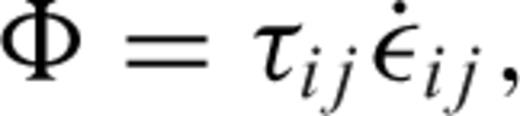
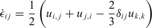
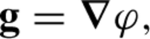
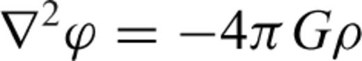
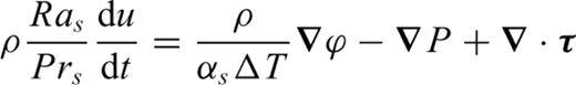
 the stress tensor, g the gravitational acceleration and ρ the density. The thermodynamic variables involved are the (absolute) temperature T, the pressure p, the specific heat cp, the thermal conductivity k and the thermal expansion α. The body force term ρg in the conservation of momentum eq. (2) describes the buoyancy forces which drive mantle flow. In convection modelling, these forces are generally assumed to arise from perturbations in density due to lateral variations of temperature inside the mantle. In the equation of energy conservation (3), the term
  describes the advection of temperature,
  the diffusion of temperature, Φ is the dissipation due to internal viscous friction,
  is the work associated with adiabatic changes of volume and the last term Q is the internal heating rate per unit volume of fluid (due to distributed radioactive energy sources in the mantle).


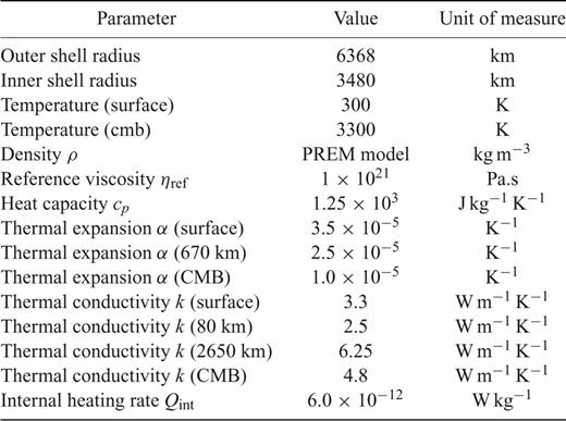
Physical parameters and values employed in simulations of thermal convection of the mantle. Values in this table were kept constant in all simulations of thermal convection of the mantle. Details of viscosity profiles are given by Fig. 1.


2.2 A spectral solution of the gravitationally consistent equations of mass and momentum conservation
As discussed above, we may solve the equations governing buoyancy-induced viscous flow in a mantle with infinite Prandtl number using a Green's function method. This approach, widely employed in tomography-based mantle flow modelling (e.g. Forte & Peltier 1987, 1991; Hager & Clayton 1989; Ricard & Vigny 1989), was first used extensively by Hager & O'Connell (1981) and is often referred to as the ‘internal loading’ formalism. The principal feature of this internal loading approach, which sets it apart from the traditional solution of momentum and mass conservation in the numerical convection models (e.g. Glatzmaier 1988; Tackley 1997), is that the solutions are obtained entirely in the spectral domain using orthonormal basis functions appropriate for spherical geometry (i.e. the spherical harmonics).
In this study, we employ the spectral method for solving the equations of mass and momentum conservation (eqs 21 and 22) in 3-D spherical geometry, using the viscosity-renormalized flow variables employed by Zhang & Christensen (1993) and Forte (2000). This spectral method provides a gravitationally consistent solution for viscous flow in a compressible spherical mantle. A similar approach was followed by Panasyuk et al. (1996). A brief overview of the method is presented here and we refer to Forte (2000) and Forte (2007) for more details.
 such that
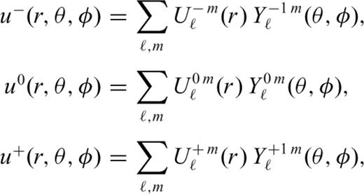

 .
.
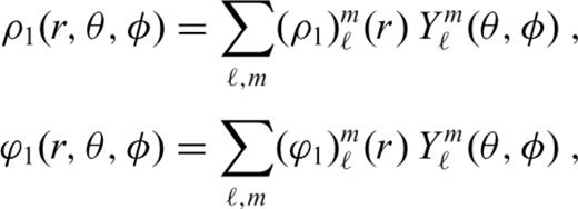
 ,
,  ,
,  ,
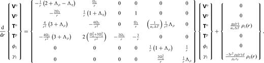
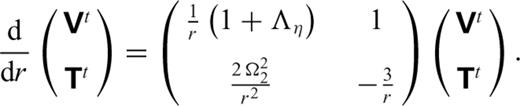
,  , φ1(r) and γ1(r) represent the spherical harmonic coefficients of vertical flow, tangential flow, vertical (radial) stress, tangential stress, perturbed gravitational potential and perturbed gravitational acceleration, respectively. These flow and stress variables characterize the purely poloidal component of the mantle flow field which is driven by the density anomalies ρ1. The generation of toroidal flow requires that the effective viscosity in the mantle vary laterally in addition to varying with depth, as assumed in the system (31). As shown below, surface tectonic plates are effectively a manifestation of lateral viscosity variations (e.g. Forte & Peltier 1994) which will generate significant toroidal flow in the (especially, upper) mantle.
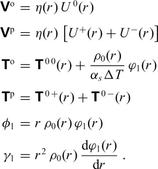
In the flow system (31) we note the dependence on viscosity is through the quantity Λη defined in (32). As shown in Forte (2000), this dependence on the logarithm of the radial viscosity profile is a consequence of the use of ‘pseudo-flow’ variables  and
and  defined in (33) and first used by Zhang & Christensen (1993). With this logarithmic dependence on viscosity, it is possible to numerically resolve extremely large variations in viscosity. This is particularly important when we consider the viscosity profiles obtained in recent geodynamic studies (Forte & Mitrovica 2001; Mitrovica & Forte 2004), which are characterized by radial variations of 3 orders of magnitude over a few hundred kilometres.
The effects of self-gravitation on buoyancy-induced mantle flow are represented by the term  appearing in the (third row, fifth column of the) flow matrix in system (31). In an incompressible mantle this coupling between gravity and flow is absent, while in a compressible mantle the perturbed gravity field deflects the level surfaces in the hydrostatic reference state giving rise to effective ‘loads’ which are superimposed on the primary driving force due to the density anomalies ρ1. The impact of these self-gravitational loads are not negligible when considering the longest horizontal wavelength components of the flow field, especially the flow-related surface observables such as dynamic topography and geoid anomalies (Forte & Peltier 1991). In particular, when considering the component of the flow field corresponding to harmonic degree ℓ=1, a gravitationally consistent solution of system (31) will ensure that the predicted ℓ= 1 component of the external gravitational potential (i.e. the dipole component of the geoid field) is zero. This result, which ensures that the centre of mass of the Earth will not be displaced, is included in our mantle convection model.
The viscous flow solution is represented in terms of Green's functions which relate the flow velocity and the stress tensor at radius r = r0 to a delta-function density load at r = r′. The system (31) is thus integrated for ρ1(r) =δ(r−r′) after appropriate boundary conditions are applied at the surface and at the core–mantle boundary (CMB; see Forte 2007, for details). Zhang & Yuen (1996) have employed a system of spectral poloidal-flow equations, analogous to those in (31), but use a finite-difference method to solve these equations for a given field of density anomalies ρ1(r, θ, φ) distributed throughout the mantle.
Tectonic plates are a fundamental part of mantle convection in the Earth and though their treatment lies beyond classical fluid mechanics theory, their dynamic impact should be modelled. A key issue in developing a procedure for coupling plates to the mantle flow field is to ensure that the plate motions, at each instant, are produced by the underlying buoyancy-driven flow and not vice versa (i.e. the ‘Hand of God’ approach in which plate motions are prescribed). This concern is especially important when modelling convection over very long time spans, for example over many hundreds of million years as presented below, because externally forced plate motions imply the addition of a non-physical energy source that is extraneous to the convecting system and this will compromise the energy balance of the mantle. We therefore employ a technique for coupling the motions of rigid surface plates to buoyancy induced mantle flow which was developed by Forte & Peltier (1991) and Forte & Peltier (1994). An alternative, conceptually distinct approach has been developed by Ricard & Vigny (1989), based on the earlier plate modelling work of Hager & O'Connell (1981). A complete mathematical description of the plate modelling theory we employ here is provided by Forte & Peltier (1994) and we will summarize only the main aspects of this method.

 are obtained through a projection operator
  as follows
 is given in Forte & Peltier (1994) and it depends on the geometry of the surface plates. The other component of the density anomalies
  is simply given by the expression
 is consistent with the geometry of possible rigid plate motions at the surface whereas the one produced by
  is orthogonal to any possible plate motion. In other words, the plates participate in the underlying flow driven by
  , while they resist the flow produced by
  . Hence, free-slip (
 ) and no-slip (
 ) surface boundary conditions are applied to model the internal flows driven by
  and
and  , respectively.
 will necessarily posses a toroidal component. This toroidal component is directly coupled to the poloidal component of the plate motions as follows
 . A free-slip condition (
 ) is applied at the CMB.
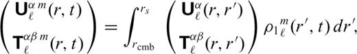
 and
and  are the generalized spherical harmonic coefficients of the velocity and stress fields (28 and 29), respectively, and
  and
and  are the corresponding Green's functions.
The Green's functions do not depend on time, nor on the azimuthal harmonic order m (owing to the assumed radial symmetry of viscosity in the mantle). In contrast, the thermally generated density heterogeneities will vary with time according to eqs (23) and (26). Hence, the Green's functions are calculated only once and then stored. At every time step, the velocity and the stress fields will be determined simply by numerically integrating the Green's functions in (40) with the time-dependent density anomalies. This approach, namely to solve the conservation of momentum equation once in terms of Green's functions, rather than solving them at every time step (e.g. Glatzmaier 1988; Zhang & Yuen 1996), is an efficient means of solving the thermal convection problem. In effect, the entire thermal convection problem has been reduced to solving one equation only: the conservation of energy equation.
2.3 Solving the equation of conservation of energy
2.3.1 Pseudo-spectral method
Several methods have been used by different authors to perform the time integration of the energy equation, the most common of which are finite differences (e.g. McKenzie et al. 1974; Jarvis & McKenzie 1980; Machetel & Yuen 1986; Solheim 1986; Larsen et al. 1997) and finite elements (Baumgardner 1985; King et al. 1990; van Keken et al. 1994; Bunge & Richards 1996; Kellogg & King 1997; van Keken & Ballentine 1999; Zhong et al. 2000). Glatzmaier (1984, 1988) employed a pseudo-spectral method and showed that, in the case of a 3-D spherical model, this method presented numerical advantages and may be less time and memory consuming. In particular, the ‘pole problem’ (Orszag 1974; Glatzmaier 1988) which arises in finite differences is absent. If the mesh used for finite differences is such that the number of longitudinal points is the same at each latitude then the distance between successive points near the poles tends toward zero. In consequence, the time step for the evolution of temperature must be extremely short in order to maintain numerical stability (see the Courant stability criterion below in eq. A28), which results in a very large number of iterations. This problem does not arise if the equations are solved in the spectral domain of the spherical harmonics. Furthermore, comparison tests between spectral and finite difference methods have been completed by several authors (Orszag 1971; Herring et al. 1974; Glatzmaier 1984) who all showed that spectral methods require fewer gridpoints, hence less memory, for achieving the same accuracy. Although, the finite element method is very flexible and does not present the pole problem, we opt for the pseudo-spectral method which is straightforward to implement (Glatzmaier 1988; Zhang & Yuen 1996).
 allows us to solve the energy conservation eq. (23) for each degree ℓ, m independently
 of the temperature field for all depths in the mantle. The relation between the coefficients and the spatial temperature field is
 into series of Chebyshev polynomials Glatzmaier (1984). This provides an accurate and efficient means of calculating the radial derivatives of temperature in (41).
The solution of eq. (41) requires us to first obtain the spherical harmonic coefficients of the terms on the right-hand side. Only the diffusion term can be calculated directly in the spectral domain of the spherical harmonics, while the advection and dissipation terms are first calculated in the spatial domain (r, θ, φ) and then transformed to the spectral domain (hence the use of the term ‘pseudo-spectral’ to describe this method). The procedure we employ to compute the different terms in physical space is simplified by using generalized spherical harmonics (Phinney & Burridge 1973) rather than ordinary spherical harmonics (e.g. Glatzmaier 1984). More details may be found in Appendix A.
2.3.2 Time integration of temperature
The numerical scheme used by Glatzmaier (1984) and Glatzmaier (1988) to perform the time integration of the energy equation is composed of two parts. The Adams–Bashforth scheme used by Glatzmaier is just the predictor part of the two-part predictor–corrector method. We instead use the complete predictor–corrector scheme in order to increase the accuracy of our results. Every iteration performing the Adams–Bashforth scheme will be followed and ‘corrected’ by an iteration performing the Adams–Moulton scheme for the nonlinear terms (advection and dissipation terms) while a semi-implicit Crank–Nicolson scheme is used for the diffusion terms. Both schemes are second-order accurate in time and they are discussed in detail by Glatzmaier (1984). But, numerical experiments (e.g. Glatzmaier 1984; Ascher et al. 1995) demonstrate that weak decay of high frequency modes can lead to appearance of aliasing in such constructed implicit–explicit (IMEX) schemes. Glatzmaier (1984) has proposed using a simple method of ‘cutting’ one half of the radial Chebyshev polynomials in the spectral domain, but with this method we lose the ability to perfectly satisfy isothermal boundary conditions.
Ascher et al. (1995) have shown that strongly damped schemes, such as semi-implicit backward differentiation formula (SBDF), modified Crank–Nicolson, Adam–Bashforth (MCNAB) or third-order SBDF can be used to inexpensively reduce aliasing. Here, we use the modified Crank–Nicolson for the diffusion terms which allows us to use the full Chebyshev spectrum. The numerical schemes employed to solve the energy conservation equation are described in detail in Appendix A4.
2.4 Determination of a geotherm—the energy balance criterion

Secular cooling provides a measure of geotherm deviation from a steady state and its value may be used to tell us: (1) how far we are from the system equilibrium at anyone moment and (2) the amount of numerical error of a determined geotherm at the end of calculation. We employ the steady-state geotherm as an estimate of the present-day geotherm in Earth's mantle, in which we underline that the total imposed internal mantle-heating rate includes both radiogenic and geologic estimates of secular cooling contributions.
3 Initial Conditions and Reference Properties of the Mantle
We use a seismic-tomography image of present-day mantle heterogeneity which satisfies both seismic and geodynamic constraints (Simmons et al. 2009) as the initial laterally varying temperature field for all simulations. This model fits 93 per cent, 92 per cent, 99 per cent and 82 per cent of seismic, gravity, tectonic plate-divergence and topography data, respectively. Also, the resolution of the original 3-D image is defined by 22 layers in the radial direction and 128 spherical harmonics in the horizontal direction.
For the purpose of this study, we use two different viscosity profiles: (1) V2-profile employed by Forte et al. (2010) and determined by jointly inverting convection-related surface observables (surface gravity anomalies, residual topography, divergence of tectonic plate motions, excess ellipticity of the CMB) and data associated with the response of the Earth to ice-age surface mass loading (decay times inferred from post-glacial sea level histories in Hudson Bay and Fennoscandia, and the Fenoscandian relaxation spectrum) and (2) ISOV-profile, that is, constant viscosity profile, η= 5.36 × 10²¹Pa.s (the depth-average value of the V2 viscosity), used to establish benchmark simulations that characterize the numerical stability of our solution scheme. The viscosity profiles are presented by Fig. 1.
Viscosity profiles. The geodynamically inferred (Mitrovica & Forte 2004; Forte et al. 2010) and V2–profile (red line) is characterized by a two order of magnitude reduction in viscosity across the uppermost mantle, where 220 km is the depth at which the V2–profile has minimum viscosity. Deeper in the mantle, there is a great increase in viscosity, about 1600×, from 635 to 2000 km depth—where the latter corresponds to the depth of maximum viscosity in the mantle. In the lower 900 km of the mantle, the V2 profile exhibits a three order of magnitude decrease of viscosity extending down to the CMB. The ISOV profile (blue line), is constant and characterizes a logarithmic average of the whole-mantle value derived from the V2 profile.
The radial density profile ρ0(r) which describes the reference hydrostatic state in our compressible convection model is taken directly from the seismic reference Earth model PREM (Dziewonski & Anderson 1981). The corresponding radial gravity field g0(r) is obtained by integrating ρ0(r).
We employ a constant heat capacity cp = 1.25 × 10³Jkg−1K−1.
The coefficient of thermal expansion α(r) is assumed to vary linearly from a value of 3.5 × 10⁻⁵K−1 at the top of the mantle to a value of 2.5 × 10⁻⁵K−1 at 670 km depth. This variation across the upper mantle approximates that found in equation of state modelling for a pyrolite mantle composition (Stacey 1998; Jackson 1998). In the lower mantle, we assume that the depth variation of α(r) follows the dependence on density (or molar volume) found by Chopelas & Boehler (1992), decreasing from a value of 2.5 × 10⁻⁵K−1 at 670 km depth to 1.0 × 10⁻⁵K−1 at the CMB.
The values of these thermodynamic input parameters are deemed to be acceptable for the upper part of the mantle by laboratory experiments and inferences from geophysical data analysis. The thermal conductivity of upper mantle is in the range 3.0–3.3Wm−1K−1. But with increasing depth our knowledge of these parameters becomes increasingly uncertain, especially for the thermal conductivity because at high temperatures and pressures the total conductivity is the sum of contributions from several independent mechanisms. In this study, we employ a thermal conductivity k, henceforth called the ‘H-profile’ that considers the effect of TBL inside the mantle and the possibility that thermal conductivity decreases with depth across both layers (Hofmeister 1999). The H-profile has k decreasing inside the upper TBL from 3.3 to 2.5Wm−1K−1 and at the top of the D″-layer k takes the maximum value of 6.25Wm−1K, while at the CMB, its value is 4.8Wm−1K−1.
As noted above in the discussion of the geotherm, we employ a total value of internal heating that is the sum of two components: radioactive sources (12 TW) and estimated secular cooling (12 TW).
The temperature increase across the mantle is 3000 K: from 300 K at the top of the mantle to 3300 K at the bottom of the mantle.
The physical parameters and values employed in the simulations of mantle convection are summarized in Table 1.
There are three types of boundary conditions that we may use for modelling thermal convection in the mantle: rigid surface (R), free-slip (F) and coupling with rigid surface tectonic plates (P). In this study, we used two of them: the R- and P-boundary conditions. P-boundary condition involves the present-day geometry of the major tectonic plates and modelling the plate-coupling to mantle flow is carried out in the no-net rotation reference frame. One important difference between them is that the P-boundary condition involves the generation of toroidal flow via the surface-plate rotations and this is not the case in either of the two other boundary conditions (R or F). Moreover, the coupling of surface plates employing the P-boundary condition requires a consideration of both rigid and free-slip flow kernels and hence this condition is, in a sense, intermediate between the R- and F-boundary conditions.
For the purpose of exploring the importance and implications of surface boundary conditions on the evolution of thermal convection in the mantle, we consider the following models: (1) the M2-HP model using V2-viscosity and P-boundary condition at the mantle top, (2) the M2-HR model defined by V2-viscosity and R-boundary condition. We will, however, begin by considering an isoviscous mantle convection simulation, the MI model, in order to validate the numerical procedures discussed above and to clarify the appropriate spatial resolution needed for so-called ‘Earth-like’ conditions.
4 Results
4.1 Numerical issues in the upper part of the mantle
The vertical resolution is defined with an order 129 Chebyshev polynomial expansion which translates into a radial-resolution length scale of 0.43km near the isothermal boundaries to 35.44km in the middle of mantle. This vertical resolution will be kept for all simulations presented in this study.
The first pair of simulations (MI-F128 and MI-N128) is based on the original MI-model and horizontally discretized by 128 spherical harmonic degrees, L = 128, giving us the horizontal spatial resolution from 85.1km at the CMB to 155.7km at the top of the mantle. The only difference between these simulations is that MI-F128 uses the isotropic linear filter (see Appendix eq. A29) applied to the spectral expansion of the nonlinear convection term over spherical harmonic degree, while MI-N128 is not filtered.
Multiplying by 10, the ISOV profile, we obtain a new model, MI×10, characterized by RaH < 109, which is used as the basis for the second pair of simulations (MI×10–N128 and MI×10–N256). Both numerical experiments, MI×10–N128 and MI×10–N256, are calculated without the filtering in the spectral domain, but with different horizontal resolution: L =128 for MI×10–N128 and L =256 for MI×10–N256.
We integrated MI-F128 over a model-time interval of 3.845 Gyr (corresponding to 36 000 time steps), and then we chose the 3-D temperature structure at that point in time to be an initial field for three remaining models (MI-N128, MI×10–N128 and MI×10–N256). Integrating all previously defined isoviscous simulations over a time window of 290 Myr, we obtained the results discussed below.
First, we note that a numerical thermal instability in the horizontal part of the spectrum developed inside the upper boundary layer from the very beginning of both L = 128 numerical experiments with no filter (Figs 2a and b). This type of instability is caused by the lack of horizontal resolution, because the MI×10–N256 model (with increased horizontal spectrum) does not generate an accumulation of energy on the shortest wavelengths (compare Fig. 2c with Fig. 2b). It seems that L = 256 provides the minimal horizontal resolution needed to solve for mantle convection defined by RaH≤ 109 without aliasing over spherical harmonic degrees. If more ‘Earth-like’ conditions correspond to RaH > 109 (most likely in the upper-mantle, where sublithospheric viscosity is lowest), this suggests that we probably have to use L≥ 512, as pointed out by Schuberth et al. (2009b).
The rms spectral amplitudes of the mantle temperature heterogeneity for isoviscous convection models after 290 Myr of time integration from the point of 3.845 Ga (see text). The rms amplitudes are represented on the Kelvin-temperature scale as a function of spherical harmonic degree (y-axis) and depth (x-axis).
Second, analysing the lower mantle, we note the absence of any numerical issues for all models (including those with no spectral filtering, Fig. 2). Therefore a valid solution for thermal convection in the lower mantle is possible even with 128 spherical harmonics degrees.
We find that filtering over a spectral domain is one of the possible solutions for controlling numerical instabilities in this study and it yields a spectrum which is free of aliasing (Fig. 2d). To justify our use of a filter, we calculated heat flux for the MI-F128 and MI-N128 simulations over a model-time interval of 3 Gyr until both simulations reached statistical steady state. The MI-F128 simulation provides a surface heat flux of 37 TW while the corresponding value of heat flux for the no-filter simulation is 40 TW. The difference of ∼3 TW is also found in the CMB flux, allowing us to conclude that filtering in the spectral domain does not affect the internal heating rate and thus the energy balance in the mantle.
It is worthwhile to explore the numerical stability of the convection model for a pair of the V2-simulations without a spectral filter and with the horizontal resolution defined by L = 256. Both systems of this pair are constructed as in the case of the initial model (MI), but with a new geotherm that is taken from the MI-F simulation at 6.85 Ga. The first V2-simulation (MV2–N256) uses the original V2-profile, while the second one (MV2×10–N256) is calculated with a viscosity 10× stiffer than the MV2–N256 model. Integrating this pair of models over 250 Myr, we notice a few interesting features. For both simulations, the location of an numerical instability, initialized by the lack of horizontal resolution, is at the depth of 220 km (Fig. 3b) where the minimum viscosity in the V2-profile is located (see Fig. 1). The stiff viscosity above 220 km depth, in the MV2×10–N256 simulation, prevents ‘noise’ transport through the lower lithosphere (Fig. 3a). The MV2–N256 does not possess this ability and the aliasing will spread through the lithosphere. Again, it is confirmed that we may be obliged to use an upper-mantle resolution corresponding to L = 512 for modelling Earth like convective flows.
The rms spectral amplitudes of the mantle temperature heterogeneity (y-axis) as a function of spherical harmonic degree (x-axis) for V2 convection models at different depths: 84 km (a), 224 km (b) after 250 Myr of time integration from the present day. The blue line remarks the MV2–N256 model and the red line shows the MV2 × 10–N256 model (see text).
For now, our numerical scheme does not have the ability to discretize layers of the mantle separately, as suggested by these results, and we employ a single whole-mantle parametrization. Although, in future studies, we may be obliged to use L≥ 512 for modelling Earth-like convective flows (at least in the upper mantle), in this study, we first wish to validate the numerical model and then to determine a first estimate of the steady state geotherm. Such simulations demand integration of more than 100000 time steps and we therefore judge that the filtered horizontal spectrum defined by 256 spherical harmonic modes could deliver a geotherm that satisfies the energy balance.
 and
and  represent their complex conjugates. From Fig. 4(b), we observe that numerical ‘noise transport’ has a transient character due to the appearance of strong advection term in thermal convection. As we already illustrated (Fig. 2), the application of a spectral filter acting over the range of harmonic degrees of the nonlinear term may be one method for controlling numerical instabilities (Fig. 4b).
(a) The rms spectral amplitudes of ℓ= 64 (y-axis) as a function of Chebyshev polynomial degree (x-axis) for the isoviscous MI-N128 (without filter) model at different points of time: 310 Ma (blue line), 410 Ma (red line) and 510 Ma (cyan line). (b) The temporal evolution of the local rms error of the predictor–corrector time-stepping method for the isoviscous simulations: MI-N128 (blue curve) and MI-F128 (with filter, red curve). The green (dashed) curve represents the logarithmic variations of total integrated kinetic energy for the MI-N128 model over 800 Myr.
4.2 Steady-state geotherm and energy balance
To determine a first estimate of the present-day geotherm satisfying bulk-energy balance, we will employ L = 256 for the horizontal resolution, using a Lanczos filter (see Appendix eq. A30) in the spectral domain, and an initial geotherm for a new set of simulations (M2-HP and M2-HR) that will be taken from the MI-F simulation at 6.85 Ga.
One of the criteria we employ to validate our numerical convection scheme is to examine the model's ability to reach and then preserve the bulk-energy balance in the mantle. We will use a 5 per cent deviation from perfect energy balance as an ‘error’ threshold to evaluate the numerical robustness of the calculated internal heating (as determined from the difference between surface and bottom heat flux).
In the first 750 Myr of the M2-HR simulation (see Fig. 5), fluctuations of internal heating are large, entering a couple of times inside the 5 per cent level and each time over a wider time interval while in the remaining 1.25 Gyr the results may be called numerically robust (as defined above). However, a standard-deviation analysis of two equal halves of the [750, 2000] Ma interval reveals that geotherm variations from 750 to 1375 Ma are still evident, especially in the bottom boundary layer (see Table 2). Thus, we defined new 5 per cent level interval, from 1375 Ma to 2 Ga (Fig. 6), where the mean heat flux at the top of the mantle is 37.24 ± 0.04 TW, and the amount at the CMB is 13.38 ± 0.05 TW. We note that the standard deviations continue to decrease during the time integration for heat flux at both top and bottom boundaries, indicating that there is no need to continue the M2-HR simulation beyond the point of 2 Ga (Table 2). The absolute mean value of numerically calculated secular cooling during the final 625 Myr interval (Fig. 7) is 0.88 ± 0.07 TW, representing the range of uncertainty in the steady-state M2-HR geotherm.
Time-dependent internal heating. The temporal evolution of internal heat production (Qc) for two convection simulations (M2-HP, with surface plates and M2-HR, with rigid surface) is calculated by differencing the heat flux at the surface (Fs) and CMB (Fc), such that Qc = Fs−Fc. The green rectangle represents a 5 per cent deviation with respect to the expected steady-state value (i.e. 24 TW of imposed internal heating), while the grey represents a 10 per cent deviation.
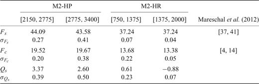
Values of mean heat flow and its standard deviations for M2-HP and M2-HR models on two equal time intervals with maximum 5 per cent deviation from true steady-state values. Evolution of heat flow on the last 625 Myr of M2-HP and M2-HR simulations is presented in Fig. 6.
Time-dependent heat flux at the surface and CMB. The top and bottom frames show temporal variations of surface (a) and bottom heat flux (b), respectively, for the M2-HP (with surface plates) and M2-HR (rigid surface) convection simulation over the final 625 Myr during which steady-state conditions prevail.
Temporal evolution of bulk cooling. The red and blue curves show the numerically determined bulk cooling of the mantle for the M2-HP (surface plates) and M2-HR (rigid-surface) convection simulations, respectively. These numerically calculated bulk cooling rates measure the extent to which the mantle geotherm departs from steady-state conditions.
The M2-HP simulation produces larger fluctuations in the heat flow compared to M2-HR (Fig. 5), but this model still satisfies bulk-energy balance in the mantle over a 1.25 Gyr interval. Using the same numerical-robustness analysis presented above, we obtained the following results for the M2-HP (with surface plates): (1) the mean values of heat flux are 43.58 ± 0.41 TW and 19.67 ± 0.38 TW for the surface and CMB flux, respectively (see Fig. 6) and (2) the estimated ‘error’ in the steady-state M2-HP geotherm is 2.60 ± 0.50 TW over the [2775, 3400] Ma 5 per cent level interval (see Fig. 7). Here, we selected the second half of the 1.25 Gyr interval to present numerically acceptable results of the M2-HP simulation (in the sense that the numerical secular cooling is minimal in this time interval, see Table 2).
Heat flow at the top and bottom of the mantle are controlled by the TBL (Figs 8a and b). The thickness of the upper boundary layer, δs, for the M2-HR model is ∼124 km while its lower boundary layer, δc, is ∼87 km in thickness. Model M2-HP (with surface plates) has thinner boundary layers: δs≈ 105 km and δc≈ 70 km.
Global horizontally averaged mantle thermal structure at the end of the steady-state interval for the M2 convection simulations.
The bulk of the mantle between the two boundary layers is characterized by an adiabatic temperature profile where advective heat transport by vertical motion dominates all other heat transfer mechanisms. The adiabatic part of the M2-HP geotherm ranges between ∼1732 and ∼2484 K indicating the evolution towards cooler bulk temperatures than the model with the rigid surface whose adiabatic values increase from ∼1824 K at the top to ∼2648 K at the bottom of the mantle. Comparing the adiabatic portions of the geotherms in both simulations with the range of values in a reference adiabatic geotherm, ranging from 1700 to 2584 K at the bottom of the mantle, estimated on the basis of mineral physics constraints that satisfy a phase-change temperature of 1800–400 km depth (Boehler & Chopelas 1991), we may say that the upper-mantle adiabat in the M2-HP geotherm is more ‘Earth-like’ than the same part of the M2-HR geotherm (2 per cent vs. 7 per cent of relative deviation), while the inverse is true for the lower-mantle adiabatic parts of both geotherms (4 per cent vs. 2 per cent).
Thus, any geotherm taken from the model time interval [1.375, 2] Ga would provide a useful starting point for the M2-HR class of model simulations, and similarly for the M2-HP models, where the acceptable 5 per cent level interval is from 2.775 to 3.4 Ga (Fig. 8c).
Time-dependent oscillations in heat flux (Fig. 6), and the corresponding variations in mantle bulk temperature (Fig. 7), are most strongly expressed in the M2-HP (surface plate coupled) simulation, owing to the larger instabilities originating in the surface boundary layer that are transmitted to the CMB via the subducting cold material. These oscillations are not characterized by any clearly defined periodicity, although fluctuations over time intervals of about 200–500 Myr are evident. Such time scales are thought to characterize the Wilson or super-continent ‘cycle’, but the assumed periodicity for this so-called cycle is uncertain, ranging from 200 Myr (e.g. Courtillot & Olson 2007) to 400 Myr (Labrosse et al. 2008). Indeed, recent analyses of global zircon data do not provide compelling evidence for a clear periodicity (e.g. Bradley 2011), while other compilations suggest that any episodicity may be characterized by longer period approaching 600 Myr (e.g. Voice et al. 2011). There are corresponding uncertainties in interpreting the surface geodynamic manifestations of this cycle, for example, in terms of surface heat flux, with as much as 30 per cent variation proposed by Labrosse & Jaupart (2007) and as little as 5 per cent proposed by Korenaga (2007). The corresponding fluctuations of heat flux at the CMB (as in Fig. 6b) have been linked to mantle plumes that trigger massive surface volcanism and also magnetic superchrons (Courtillot & Olson 2007). As noted by Courtillot & Olson (2007), even small fluctuations in CMB heat flux, near a critical threshold value, can lead to changes in magnetic reversal frequency. Perhaps the most relevant result is the hemispherical style of convection that ultimately develops in the M2-HP model (discussed below), a pattern that has been identified as intrinsic to the cycle of super-continent formation and dispersal, as modelled for example by Yoshida & Santosh (2011) and Zhong et al. (2007).
4.3 Lateral heterogeneity and flow patterns
In the first 65 Myr, both model simulations maintain the initial amplitude of the dominant convection modes in the range, ℓ∈ [1, 16] (Fig. 9a). The strong subduction zones, reinforced in the first 30 Myr and the plumes of the M2-HP simulation extend across the mantle to the opposite thermal boundary layer (TBL) after 65 Myr and the consequent mixing of this transported thermal heterogeneity inside the boundary layers has commenced (Fig. 9a). In the M2-HP simulation, a strong ℓ= 1 mode is established inside the adiabatic part of the mantle between 110 and 525 Myr (Figs 9b and c) and the evolution of the temperature structure in the TBL is completed at about 820 Myr (Fig. 9d). At this time, the predominance of amplitudes associated with ℓ= 1 spans the entire mantle and remains stable through the interval of steady-state conditions (Figs 9e and f). The dominance of degree 1 convection in terrestrial mantles has been revealed in past explorations of so-called ‘stagnant-lid’ convection (Roberts & Zhong 2006) and convection with strong lateral viscosity variations (Yoshida 2008).
Time-dependent evolution of lateral temperature variations driven by mantle convection. In the top two rows are shown equatorial cross-sections of evolving temperature heterogeneity from 65 Ma (on the left), estimated from seismic tomography (Simmons et al. 2009), to 2 Ga into the future (on the right). The 1st and 2nd rows show the M2-HP (surface plates) and M2-HR (rigid surface) results, respectively. The bottom (3rd) row shows the dominant mode of convection (i.e. maximum spectral amplitude of thermal heterogeneity) as a function of depth at each instant in time.
The primary characteristic of the M2-HP simulation is the intense reinforcement, in the starting tomography model, of subducted material that enters the mantle under the Indonesian and Western Pacific trench systems. Starting with the tomography-derived thermal structure ensures that this initial trajectory is strongly imprinted on the future evolution, since the present-day flow field is marked by strongest subduction, globally speaking, in this region. The time-dependent evolution of this subduction ultimately leads, over the billion-year interval examined here, into a dominant hemispherical configuration of temperature anomalies in the mantle. This evolution is, of course, affected by the time-invariant surface plate geometry employed in this simulation. It is important to recall however, especially from the perspective of dynamic and energetic self-consistency, that the surface plate motions are not forced with imposed (prescribed) velocities in the plate-coupled flow calculations. This differs from previous approaches involving a prescribed history of surface plate velocities (e.g. Zhang et al. 2010). Although the geologically inferred dominance of subduction along the margins of the palaeo-Pacific (e.g. Zhang et al. 2010) may suggest that this hemispherical pattern of subduction is not unreasonable, we do not suggest that a fixed billion-year pattern of surface subduction is tenable. We instead choose to run these simulations to steady state to quantify the mean (ℓ= 0) thermal structure (i.e. geotherm and heat flow) in the mantle. The time-dependent evolution of lateral heterogeneity over the first 100–200 Myr is of primary interest in exploring the interaction of subducting material with the very large radial increases of mantle viscosity as well as the amplification and propagation of the upwelling plumes from the lowermost mantle (discussed below).
In contrast to convection with moving surface plates, the M2-HR (rigid-surface) simulation does not generate ‘giant’ subductions zones and the downward sinking mantle originating in the cold, upper TBL is characterized by relatively weak-amplitude thermal anomalies. The changing structure of the upper TBL, due to the impact of ascending thermal plumes, continues to evolve until 525 Ma (Fig. 9c) and beyond this point the dominant modes of convection are characterized by harmonic degrees ℓ= 3 and 4 (Figs 9d, e and f).
The M2-HR (rigid surface) simulation reveals the remarkable stability and very long-term longevity of mantle plumes that originate in the starting 3-D tomographic image of hot-mantle anomalies inside the D″-layer (Fig. 10a).
The first map (a) shows the present-day positive heterogeneity (T≥ 100 K) at the depth of 2650 km. The maps from (b) to (f) represent positive lateral temperature variations (T≥ 100 K) at the depth of 220 km obtained by the M2-HR (rigid surface) convection simulations at different points/intervals of time: 200 Ma (b), 205–400 Ma (c), 405–600 Ma (d), 605–800 Ma (e) and 2 Ga (f). The black circles show the location of present-day hotspots (Courtillot et al. 2003).
The steady-state plumes appear at the depth of 220 km during first 200 Myr (Fig. 10b). We note that four of five plumes that remain stable up to 2 Ga (Fig. 10f) may be linked with the locations of the present-day hotspots (Courtillot et al. 2003). The first cluster of hotspots is located around the edges of a plume that originated under East Pacific Rise (see Table 3). The origin of the second plume is between Fernando and Cape Verde hotspots associated with the South American and African plates, respectively, that is, located at the mid-Atlantic ridge. The Crozet hotspot related to the Antarctica Plate is relatively close to the centre of the third plume (44°S 56°E) that also could be the source of Kerguelen, Marion and Reunion hotspots. We also note the isolated Caroline hotspot that could be connected to the Darwin Rise—a large region of anomalously shallow bathymetry in the Western Pacific (Cadio et al. 2011). The location of a fifth plume under the European part of Northwest Russia cannot be related with any present-day hotspot. Although the origin of this ‘Siberian’ plume (Smirnov & Tarduno 2010) is beyond the scope of this paper, the ability of the convection model to ‘capture’ and reinforce this plume in the diffuse lower-mantle signal present in the starting tomography model is intriguing.
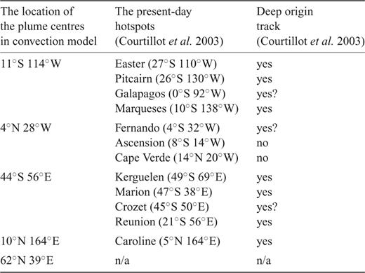
The location of the plume centres obtained by theM2-HR simulation at t = 2 Ga (Fig. 10) that may be connected by the present-day hotspots with its indicator of deep origin track.
From Figs 10(c), (d), and (e), we observe that other major hotspots have transient appearance, while some of them are not detectable by the M2-HR model (see Table 4). Also, it seems that during one period of time around 200 Ma (Fig. 10b) Iceland hotspot is part of the super plume which is subsequently re-organized into the ‘Siberian’ plume.
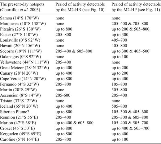
The location of present-day hotspots, and the approximate time interval of their appearance at the depth of 220 km for both convection simulations (M2-HR and M2-HP) during first 800 Myr.
In contrast to the M2-HR model, the M2-HP (plates) convection simulations cannot yield stable and very long-term longevity mantle plumes (Fig. 11). But, the M2-HP model is able to track the evolution of Marqueses, Louisville, Hawaii, Galapagos, and Martin hotspots that are undetectable by the M2-HR (see Table 4). The detection of the hotspots-related plumes is only possible up to 820 Ma because after that, the pattern of steady-state convection for the M2-HP model is dominated by the degree 1 (see Fig. 9).
The superimposed 5-Myr time sequences of positive heterogeneity (T≥ 100 K) at the depth of 220 km obtained by the M2-HP (plates) model at different time windows (Ma): 0–100 (a), 105–200 (b), 205–300 (c), 305–400 (d), 405–500 (e), 505–600 (f), 605–700 (g) and 705–800 (h). The black circles show the location of present-day hotspots (Courtillot et al. 2003).
The M2-HP (plates) simulation shows more fluctuations in the lateral variations of temperature (Fig. 12a) that precede by a couple of tens of Myr the geotherm perturbation (Fig. 12b). The fluctuation are also of larger amplitude (Fig. 13) because of the effects of changing subduction of cold material at the surface that have an ability to transport perturbations deep into the lower mantle and reaching the CMB (see Fig. 9). In contrast, the M2-HR simulation is dominated by the dynamics of ascending hot plumes and these are much more steady than subducting material. However, the variations in mantle thermal anomalies that provide the buoyancy changes reflected in the kinetic energy precede by a couple of hundreds of Myr the geotherm perturbations seen in the heat flux difference (Figs 12c and d).
The temporal variation of total integrated kinetic energy (Ek) in the surface plates (a) and rigid-surface (c) convection simulations. It seems that the fluctuations of kinetic energy (red curve) and the estimated internal heating (Qc, grey curve) are closely coupled. Making a sequence of coupled maximum values for Ek (blue circles) and Qc (green circles) over successive time windows up to 2–1 Ga for the M2-HP and M2-HR models, respectively, we can calculate the difference between the moments of maximum as a function of sequence member, (b) and (d).
Globally averaged, rms amplitude of lateral temperature variations as a function of depth. The green curve shows the present-day rms temperature anomalies derived from seismic tomography (Simmons et al. 2009). The red and blue curves shows the steady-state temperature anomalies for the M2-HP (surface plates at time 3.4 Ga) and M2-HR (rigid surface at time 2 Ga) convection simulations, respectively.
Although the M2-HP or the M2-HR simulations are not expected to be representative of the actual evolution of Earth's mantle into the distant future, we conjecture that the convective trajectory of the ‘real’ Earth may lie between these two end-member cases. From a purely fluid-mechanical perspective of instantaneous (present-day) flow, the surface boundary on a planet with a limited number of tectonic plates is not far from a no-slip surface (e.g. Ricard & Vigny 1989; Forte & Peltier 1994). This result follows from the very limited number of surface degrees of freedom (3 ×N), for N plates, relative to the effectively infinite number of degrees of freedom (e.g. the harmonic coefficients of the mantle flow field) for the underlying convective flow. So for this reason, the evolution of the M2-HP and M2-HR simulations is similar in the first few millions of years. Obviously over billion-year time scales, the differences accumulate and the two simulations ultimately diverge. We note however, from a comparison of Figs 10 and 11 for M2-HR and M2-HP, that the stability and evolution of the main hot upwellings in the mantle is similar over the first ∼200 Myr. These results suggest to us that the present-day tomography models resolve plume structures that may be remarkably stable and long-lived over timescale scales of (at least) several hundred Myr. It is notable that this stability does not require the assumption of thermochemical piles in the lower mantle (e.g. McNamara & Zhong 2005), but rather arises from the stabilizing influence of the geodynamically constrained lower-mantle viscosity structure we employ (e.g. Forte & Mitrovica 2001).
5 Discussion
We have developed a pseudo-spectral numerical model of compressible, gravitationally consistent, thermal convection in a spherical-shell planetary mantle that is capable of delivering accurate and robust solutions over very long geological times scales (involving several hundred thousand numerical time steps). For Earth-like Rayleigh numbers, we find that a fully resolved solution of thermal convection dynamics in the upper mantle may require a horizontal expansion of the field variables up to spherical harmonic degree 512 (corresponding to a horizontal resolution scale of less than half a degree on the sphere). In contrast, for a fully resolved description of convection dynamics in the lower mantle, we find that a spherical harmonic truncation level at degree 128 is entirely sufficient. These differences in depth-dependent numerical resolution are consequences of the radial viscosity profile of the mantle that is constrained by surface geodynamic data, in which the average viscosity of the lower mantle is nearly two orders of magnitude greater than average upper-mantle viscosity.
To reconcile the contrasting horizontal resolution requirements in the upper and lower mantle, we have adopted a globally uniform spectral description characterized by a spherical harmonic truncation at degree 256. To control any possible numerical instabilities in the upper mantle due to aliasing in the spectral domain we employed a Lanczos filtering of the spherical harmonic expansion of the nonlinear temperature advection term. We found that the application of this spectral filtering throughout the mantle did not bias the essential global energy balance, a criterion we systematically applied to verify the numerical accuracy of our solutions. More specifically, our numerical validation of the mantle convection solutions reveals that we can achieve and preserve a steady-state global energy balance (to within 5 per cent) over very long geological time intervals (beyond 2 Gyr or 50000 time steps) for both plate-like and rigid surface boundary conditions.
We obtained a valid approximation of steady-state geotherms for both surface boundary conditions (tectonic plates, rigid surface). In both cases, we obtain surface heat flux values in the range of Earth-like values: 37 TW for a rigid surface and 44 TW for a surface with tectonic plates coupled to the mantle flow. Past estimates of CMB heat flux have been based on a number of different methods (see Jaupart et al. 2007; Mareschal et al. 2012) with values ranging widely between 4 and 14 TW. Currently, the highest estimates of CMB heat flux have been derived from models of the post-perovskite phase transition at the base of the mantle, with values of at least 13 ± 4 TW (e.g. Lay et al. 2006). We find, therefore, that although our convection simulations deliver relatively high CMB heat flux, namely 13 TW and 20 TW, for rigid and plate-like surface boundary conditions, respectively, these values are compatible with the independent higher estimates cited above. We further note that the relatively high values of CMB heat flux predicted by our convection models are obtained assuming a CMB temperature of 3300 K. If we employ higher CMB temperatures, for example 4000 K (Boehler 1996), then our predicted CMB heat flux becomes much larger than even the current highest independent estimates. The CMB temperature is therefore an important controlling parameter and this issue is discussed further below.
We have also found, for a rigid-surface boundary, that the dominant modes of steady-state convection that persist over very long time scales correspond to harmonic degrees 3 and 4. It is interesting that these same modes were also identified as dominant by Chandrasekhar (1961) the basis of his solutions of the marginal stability problem for convection in spherical shells. The dominant convection modes for the rigid-surface simulations are able to reinforce and maintain the stability of some of the present-day hotspot-related plumes in the mantle and this stability extends over remarkably long geological time spans (of order 1 to 2 Gyr).
The plate-like surface boundary condition, in which the tectonic plate motions are coupled to those inside the mantle, is also able to produce some of the hotspots but these hotspot-related plumes are transient in character, persisting over the first few hundred million years (see Fig. 11), but then continue to change in pattern after about five hundred million years as the model evolves further to long-term steady state.
The plate-like surface boundary condition yields a dominant mode of steady-state convection characterized by the long-term stability of two hemispherical structures, one hot and another cold where the latter contains giant descending limbs of cold subducted material that extends down to the CMB. We note, however, that prior to steady state, the M2-HP simulation shows a temporal evolution through several distinct regimes. During the initial period, over the first 110 Myr, the slab and plume structures in the starting tomography model are reinforced due to the build-up of heterogeneity in the top and bottom TBLs. Between 110 and 525 Ma, a strong ℓ= 1 mode is established within the adiabatic interior of the mantle, outside the TBLs, and in the next 300 Myr, a clustering of subduction and upwelling occurs, thereby forming two opposing thermal hemispheres.
The dominance of such a degree 1 pattern of convection has been found in previous studies that included moderately strong lateral viscosity variations (Yoshida 2008). Our current implementation of the pseudo-spectral method does not explicitly model the effect of lateral variations in viscosity (LVV). The impact of such LVV has been previously explored in a number of studies of instantaneous mantle flow, for cases in which the LVV are focussed in the lithosphere or alternatively in the lower mantle (e.g. Čadek & Fleitout 2003, 2006; Tosi et al. 2009) and in cases where they are distributed throughout the mantle (e.g. Forte & Peltier 1994; Moucha et al. 2007) showed the amplitude of the dynamic effect of the LVV on surface observables is of the order of that due to differences (i.e. uncertainties) among the different seismic tomography models.
While surface observables appear to be relatively insensitive to LVV, the internal buoyancy-driven flow may be significantly affected, such that hot upwelling plumes may be more strongly focussed, with amplified flow velocities inside the main upwellings. This LVV enhancement of mantle plumes is based on the standard assumption that thermally activated creep is the only dominant mechanism that is relevant in the mantle. If so, the LVV will also have an effect at the bottom of the mantle, such that the D″-layer will be more unstable and generate plumes with greater frequency. The outstanding issue is then how to incorporate a representation of LVV in convection models that is at the same time compatible with mineral physics and with surface geodynamic constraints on mantle rheology. Current efforts to include LVV in time-dependent convection models (e.g. Nakagawa & Tackley 2008; Zhang et al. 2010) are based on simplified representations of both the depth (pressure) and temperature dependence of viscosity. None of these parametrized LVV models have been shown to generate a satisfactory fit to the range of geodynamic surface observables that have been considered in past 1-D inversions of these surface data (e.g. Mitrovica & Forte 2004). These difficulties are further exacerbated by the recognition that temperature (and pressure) is not the only contributor to LVV and that chemical effects (e.g. hydration state), variations in grain size (e.g. Solomatov & Reese 2006) and variations in deformation mechanisms (e.g. Cordier et al. 2012) can have equally important (and possibly stronger) effects. In other words, there is a great deal of uncertainty regarding the appropriate representation of LVV in mantle convection models. Confronted by these major uncertainties, we have opted to work with depth-dependent viscosity profiles that have been directly verified against a wide suite of geodynamic surface constraints (Mitrovica & Forte 2004; Forte et al. 2010) and independent mineral-physical modelling (Ammann et al. 2010). In this study, we regard the incorporation of rigid, but mobile (free rotating) surface plates overlying a very low viscosity asthenosphere in model M2-HP as effectively equivalent to extreme LVV at the top of the mantle.
One major simplification in the convection model with surface plates (M2-HP), is the assumption that plates retain their present-day configuration over very long (billion year) time spans. We know from geological reconstructions that plate geometries have constantly evolved over the past 200 million years (e.g. Müller et al. 2008), although the large-scale pattern of long-term circum-Pacific subduction seems rather stable. There is, on the other hand, no currently accepted theory for accurately predicting the future evolution of surface plate geometries over very long geological time spans, in a manner that is dynamically self-consistent with the underlying mantle flow. It is this difficulty that also led us to explore long-time convection simulations with a simple rigid surface (an ‘one-plate’ model), to avoid the possible geometric and dynamic bias of assuming fixed surface locations for subducting cold material in the mantle. The existence of substantial hemispheric-scale cold material descending to the CMB and its enhanced cooling of the mantle, appears to be the main explanation for higher surface heat flux (by 7 TW) compared to the rigid-surface (M2-HR) convection solution where the primary mode of heat transport across the lower mantle is via the hot and stable upwelling plumes producing a heat flux in the range of acceptable values.
Although it is therefore clear that our convection modelling is an undoubtedly simplified representation of the complex nature of the dynamics in Earth's mantle, it is useful to recall the importance of some of the novel aspects of our numerical simulations.
First, we used a ‘realistic’ viscosity profile (V2), determined in previous inversions (Mitrovica & Forte 2004; Forte et al. 2010) of geodynamic data sets that constrain the rheology of the mantle, which is characterized by radial changes in η over three orders of magnitude. Some previous mantle convection studies in spherical geometry (e.g. Schuberth et al. 2009b) have used simplified (2 or 3 layer) radial viscosity structures, not directly derived from geodynamic constraints, and the resulting heat-flux predictions differ from those presented above, even though other input parameters are similar. There are outstanding uncertainties in the geodynamically inferred mantle viscosity, particularly in the lowermost mantle (e.g. in the D″-layer) where the constraints are weakest (Forte 2007). For example, Steinberger & Calderwood (2006) calculated instantaneous mantle flow, assuming the thickness of D″ to be 200 km, and obtained a viscosity profile constrained by mineral physics (melting temperatures) and surface observations. This viscosity profile is characterized by strong increase with depth in the lower mantle, up to about 1 × 10²³ Pa.s above the D″ layer, and more than 100× viscosity reduction within the lowermost 200 km (D″ layer). Comparing with the V2-profile, the viscosity obtained by Steinberger & Calderwood (2006) is less than 10× stiffer inside the D″ layer thereby yielding a thicker lower TBL, and thus lower CMB flux than we simulated here. Obviously, the assumed mantle viscosity structure has a critical impact on the spatial (and temporal) evolution of mantle temperature variations, especially since each viscosity profile is characterized by local, depth-dependent RaH that vary over several orders of magnitude.
Second, we employ a thermal conductivity that varies with depth according to recent mineral physical calculations (Hofmeister 1999) and takes into account the thermal structure of the boundary layers at the top and bottom of the mantle. The assumed depth-dependence of thermal conductivity is of major importance inside the TBL, because heat transfer by conduction is either dominant or roughly equal to heat transfer by advection. A widely assumed choice for thermal conductivity in previous mantle convection models is the use of a constant value (typically, k = 3Wm−1K−1). The assumption of such a constant value of conductivity is within the range of Hofmeister (1999),k-profile for the oceanic lithosphere, but about 2× lower for the D″-layer and thereby explains previous predictions of lower CMB heat flux (e.g. Schuberth et al. 2009b) than is estimated in our study.
An outstanding question in current mantle convection modelling is the appropriate value for the temperature at the CMB, which depends on knowledge of the adiabatic temperature profile in the outer core. Improved mineral–physical constraints on the CMB temperature, and hence the temperature jump across the D″-layer, can therefore provide independent information on the heat flux at the CMB. In previous mineral–physical modelling by Boehler (1996) it was estimated that the temperature jump across the CMB is 1400 K, constrained by a minimum temperature on the core side of the CMB of 4000 ± 200 K and a mantle temperature at the CMB of about 2600 K. This estimate of CMB temperature is obtained using the adiabatic temperature drop across the liquid core of 850 K, pinned to an estimated temperature at the inner core boundary (ICB) of about 5000 K, estimated from iron melting data (Boehler 1996).
We note that the CMB temperature of 3300 K employed in our mantle convection simulations, although lower than the earlier estimates from laboratory and mineral–physical data (e.g. Boehler 1996), was necessary to obtain acceptable value of surface heat flow and to avoid excessively large CMB heat flux and mean mantle temperatures. It is therefore of some interest that recent laboratory data on the melting of iron at core conditions, in the presence of other light elements (e.g. S and O) now suggest that the outer core adiabat may be substantially cooler than previously estimated, and that our assumed CMB temperature may be plausible, if still on the lower end of the currently estimated range (Huang et al. 2011; Terasaki et al. 2011). Closely related to the question of CMB temperature, and the energy budget of the mantle, is the rate of secular cooling and, in particular, the radial distribution of internal heating. These outstanding questions provide motivation for a new set of simulations that will be tested in future studies employing the robust and efficient numerical convection methods presented in this work.
In summary, there are two basic findings which emerge from the very long-time scale, tomography-based convection simulations presented above. The first concerns the extent to which a ‘memory’ of the pattern of mantle heterogeneity in the starting tomography model is preserved over time. We find that with both the M2-HP and M2-HR convection simulations, there is a remarkable persistence of the hot, plume-like structures originating in the deep lower mantle. Indeed, there is no a priori reason to anticipate that the plumes resolved in the starting tomography model should be maintained over very long times, especially in the high Rayleigh number regime that characterizes our convection models. Moreover, these simulations do not include dense chemical ‘piles’ at the base of the mantle that have been assumed necessary for stationary plumes (e.g. Tan et al. 2011). The geographic stability of the deep–mantle plumes is found to extend over the first few hundred Myrs in the M2-HP (plate coupled) model and for even longer in the M2-HR (rigid surface) model. This plume stability and longevity is dependent on the important rheological stabilization (e.g. Lowman et al. 2004, 2008; Quéré & Forte 2006) associated with the very high lower-mantle viscosity peak inferred from geodynamic constraints (Forte & Mitrovica 2001; Mitrovica & Forte 2004). As shown in Figs 10 and 11, the most stable and long-lived deep-mantle plumes show an intriguing spatial relationship to the surface constellation of hotspots and other manifestations of intraplate volcanism (e.g. Siberian traps). The second result to emerge from our exploration of very long-time scale convection is the high heat flux that obtains at the CMB, thereby providing the thermal energy that maintains the vigour of the deep-mantle plumes. There is indeed a direct and necessary connection between high heat flux and the strength of the lower-mantle plumes (e.g. Schuberth et al. 2009b). Finally, although some convection studies have argued that large-amplitude chemical heterogeneity in the lower mantle (e.g. Tan et al. 2011) is needed to generate stable plume groups, our results suggest that the geodynamically constrained viscosity maximum in the lower mantle, in conjunction with high CMB heat flux, is very effective in maintaining long-lived stable plumes. Indeed our findings ultimately lend further support to previous studies demonstrating a dominantly thermal interpretation of heterogeneity in the tomography models (e.g. Forte & Mitrovica 2001; Quéré & Forte 2006; Simmons et al. 2007, 2009; Schuberth et al. 2009a,b; Davies & Davies 2009).
Acknowledgments
A.M.F. is grateful for the support of this work provided by the Natural Sciences and Engineering Research Council of Canada and by the Canadian Institute for Advanced Research (Earth System Evolution Program). The simulations used in this study are computed on the supercomputing facilities of the SciNet consortium at the University of Toronto. We thank the staff of the SciNet for their support. Also, we thank the reviewers for their stimulating comments and suggestions. [Correction made after online publication 2012 June 27: addition of last sentence of the Acknowledgments.]
Appendices
Appendix A: Pseudo-Spectral Numerical Solution of the Energy Conservation Equation
This section describes the procedure employed to obtain the spherical harmonic coefficients of all terms involved in the equation of conservation of energy (41).
A1 Diffusion operator
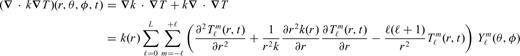
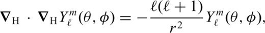
 is the horizontal gradient. We note that relation (A1) is valid when the thermal conductivity k depends only on r, as we assumed in section 3. The spherical harmonic coefficients in (A1) depend on the radial derivatives of the temperature. These derivatives are readily calculated from a Chebyshev polynomial expansion of the radial dependence of the harmonic coefficients of the temperature,
  .
.
 .
.

 are known polynomials function of depth, their derivative is also known.
The choice of Chebyshev polynomials is not fortuitous as they present two main advantages (Glatzmaier 1984). First, Chebyshev functions provide the best polynomial interpolation due to their favourable convergence properties. Secondly, the Chebyshev grid is formed of non-equally spaced nodes with a greater number at both extremities of the interval. This characteristic results in a higher resolution in the boundary layers which is beneficial because the boundary layers are the main sources of convective instabilities.
A2 Advection
The nonlinearity of the advection term makes its spectral representation challenging. This term cannot be easily expressed in the spectral domain without having recourse to cumbersome spherical harmonic coupling coefficients (e.g. Forte & Peltier 1994). It is more readily calculated in the spatial domain (r, θ, φ) where the temperature gradient, the velocity field and their scalar product may be easily determined. The latter is then transformed to the spectral domain of the spherical harmonics. The procedure we employ to compute the different quantities in the spatial domain, using generalized spherical harmonics (Phinney & Burridge 1973), differs from the one described by Glatzmaier (1984).
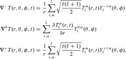
 are the components of the temperature gradient in the complex spherical basis (e−, e0, e+) defined by eq. (27).
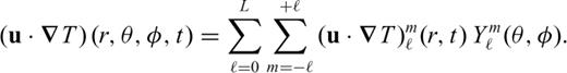
 are determined numerically by integration on a spatial geographic grid via the use of FFT's and Gauss-Legendre integration. They will be used for the solution of eqs (41).
A3 Dissipation and internal heating
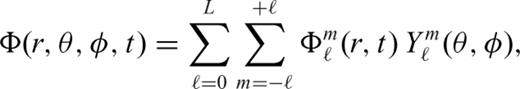
 are determined via the use of FFT's and Gauss–Legendre integration.
A4 Solution of the equation of energy conservation
Numerical scheme

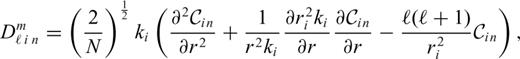
 .
.If we assume that time integration interval is discretized, j = 0,…, M, and the solution is known at time tj and tj− 1, then the numerical scheme employed to compute the solution at time tj+ 1 is described by the following equations:
- •Predictor (nonlinear terms) + modified Crank–Nicholson scheme (diffusion)(A18)

- •Corrector (nonlinear terms) + modified Crank–Nicholson scheme (diffusion)(A19)

Δtj− 1 and Δtj are two successive time steps; the time step varies according to the Courant stability criterion described by eq. (A28) below.  represents the predicted temperature at time tj+ 1 and before correction,
  is the corresponding predicted nonlinear term.
The above procedure can not be employed for the first iteration because it requires the solutions at two successive time steps. Therefore, the following SBDF (semi-implicit backward differentiation formula) scheme is employed for the predictor–corrector method for the first iteration
- •Predictor scheme(A20)

- •Corrector scheme(A21)

Thermal boundary conditions
The previous eqs (A18) to (A21) are used at each depth ri,i = 1,…, N− 1, (N+ 1) being the number of Chebyshev points. At the surface r0 and at the CMB rN, boundary conditions are required. There are two types of boundary conditions which can be used, either isothermal boundary or constant heat flux. Isothermal boundaries seem to be more realistic for both the Earth's surface and the CMB, and yet several authors (e.g. Solheim 1986; Jarvis 1991) have opted to apply a constant heat flux condition to model the CMB. This allows one to control the ratio of flux coming from the core to the one induced by internal (radioactive) heating. In this study we have employed isothermal conditions for both the surface and the CMB.
 , we are left with
Solution of the system
There are L(L+ 1)/2 systems of form (A27) to be solved where L is the maximum degree of the spherical harmonic expansion. Since Ain does not depend on m (see eq. A16), there are only L matrices to be inverted. The LU decomposition method is used to invert the matrices. The decompositions may be stored because the Ain's do not depend on time. However, they depend on Δt which may vary due to numerical stability requirements (see eq. A28) and we must therefore recompute the matrices.
The solutions Xn of the systems (A27) are the Chebyshev and spherical harmonic coefficients of the temperature  . These coefficients will be used to recompute the new radial derivatives as in (A5) needed for the evaluation of the spherical harmonic coefficients of the diffusive term in (A6) and in the calculation of
  in eq. (A7). Then, the spherical harmonic coefficients
  will be synthesized at every depth to evaluate
  and
and  in (A7).
Numerical stability requirements
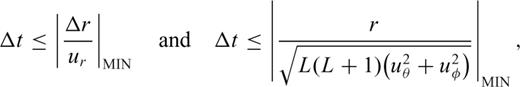
Alias-free transformations
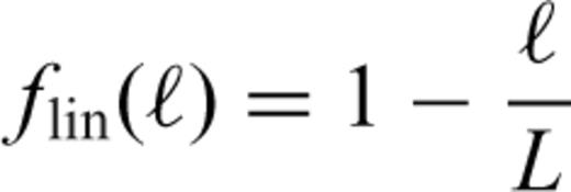
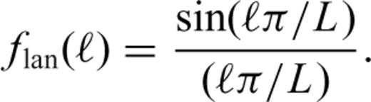
Appendix B: Computational Aspects of the Numerical Code
The thermal convection code utilized for all calculations presented in this paper is written in standard C++ language. The Blitz++ library is used for the management of large multidimensional arrays in order to be competitive with Fortran90 performances. The MPI-2 library is employed for the purpose of parallelization of the code for use on a multiprocessor computer cluster. The parallelization is mostly done over radial and latitudinal nodes and only the predictor–corrector method is distributed to processors over spherical harmonics degrees. In this way, we avoided a lot of communication between processors. Although this strategy yields gain in speed, we must deal with the limitation of the fixed size of dynamic memory available on each processor, which obviously does not increase with the size of the cluster (see Table B1). This limitation currently prevents us from using harmonic expansions up to L = 512 because we then require more than 4 Gb per processor. All simulations are done on the General Purpose Cluster (GPC) of the SciNet consortium at the University of Toronto, using Infiniband network where each node has 8 processors and the RAM per node is 16 Gb.
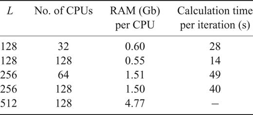
Computational properties of the numerical convection code.
References
