The signature of depth-dependent viscosity structure in post-seismic deformation

Summary

1 Introduction

Development of satellite-based geodetic observations (GPS and/or InSAR) has allowed us to accurately measure real-time surface deformation caused by subsurface geological processes such as earthquakes and/or magmatic intrusions (e.g. Hager et al. 1991; Massonnet & Feigl 1998). However, the observed data may represent the integrated effects of several mechanisms. Quantitative modelling studies are, therefore, essential in attributing an observed deformation pattern to a particular driving mechanism or to some combination of different mechanisms (e.g. Pollitz et al. 1998; Hearn 2003; Freed & Bürgmann 2004; Freed et al. 2006b; Chang et al. 2007; Ryder et al. 2007; Hearn et al. 2009; Tizzani et al. 2009; Barbot & Fialko 2010).

The surface deformation following an earthquake has been explained by noting that the elastic stress redistribution associated with fault slip is relaxed by several mechanisms, including afterslip (e.g. Bürgmann et al. 2002; Ergintav et al. 2002; Hearn et al. 2002, 2009; Ryder et al. 2007; Hashimoto et al. 2008; Suito & Freymueller 2009), poro-elastic relaxation (e.g. Peltzer et al. 1998; Fialko 2004) and/or viscous relaxation (e.g. Nur & Mavko 1974; Williams & Richardson 1991; Hearn 2003; Hetland & Hager 2003; Freed & Bürgmann 2004; Ryder et al. 2007; Freed et al. 2010). Because observed post-seismic deformation reflects the integrated effect of these mechanisms, it is necessary to quantitatively evaluate each relaxation process to understand its contribution to observed post-seismic deformation.

Among the several post-seismic deformation mechanisms, viscous relaxation may dominate the long period and long wavelength components of deformation. Comparison of observations with the linear Maxwell viscoelastic model (constant uniform viscosity [UNV] beneath an elastic upper layer) has revealed that the relaxation of post-seismic deformation is characterized by multiple timescales; greater viscosities are inferred in the later phases of relaxation (e.g. Pollitz 2003, 2005; Freed & Bürgmann 2004; Ryder et al. 2007; Hearn et al. 2009). The differences between the geodetic observations and the model predictions have been explained by complex rheological models, including the standard linear solid model (e.g. Cohen 1982; Hetland & Hager 2005; Ryder et al. 2007), the biviscous Burgers model (e.g. Pollitz 2003, 2005; Hetland & Hager 2005, 2006; Pollitz et al. 2006, 2008; Hearn et al. 2009) and the triviscous viscoelastic model (e.g. Hetland & Hager 2005).

A stress-dependent viscosity (i.e. a power-law rheology model) has also been invoked to explain the observed rates of decay of post-seismic deformation (e.g. Williams & Richardson 1991; Freed & Bürgmann 2004; Freed et al. 2006a). In this kind of model, the apparent spatial and temporal variations of viscosity are generally consistent with observation. Models with a depth-dependent viscosity (DDV) structure can also predict multiple timescales of viscous relaxation (e.g. Hetland & Hager 2006; Riva & Govers 2009). Other authors have constructed models with several viscosity layers, resulting in a range of viscosity estimates for the lower crust and upper mantle which match specific geodetic observations (e.g. Pollitz et al. 1998; Hetland & Hager 2003; Vergnolle et al. 2003).

Spatial variation of the viscous creep parameter is probably an essential element of any successful model of post-seismic relaxation because of the strong temperature-dependence of creep deformation (e.g. Goetze & Evans 1979; Kirby 1983; Carter & Tsenn 1987; Kohlstedt et al. 1995; Ranalli 1995). The lithospheric temperature gradient is typically ∼10–30°C km^–1 (e.g. Turcotte & Schubert 1982). The resulting depth-dependence of viscosity produces a first-order effect, which must be carefully evaluated to assess whether a Maxwell-type constitutive law (in which elastic and viscous strain rates are simply additive) is adequate, or if a more complex representation of the viscoelastic constitutive mechanism (e.g. Burgers model, or stress-dependent viscosity) is required.

In this study, using a 3-D finite element model, we compare the response to an instantaneous strike-slip fault of a linear Maxwell viscoelastic layer with a DDV structure to that of a constant UNV model. The DDV structure used in this study differs from previous multilayer models (e.g. Pollitz et al. 1998; Hetland & Hager 2003, 2006; Vergnolle et al. 2003); we define the creep viscosity here to have an exponential dependence on depth [as also used by Katagi et al. (2008), Riva & Govers (2009) and Takeuchi & Fialko (2012)]. This model represents approximately the effect of temperature increasing with depth, simplified to facilitate exploration of the relevant parameter space.

We first describe the general behaviour of UNV and DDV models. Then we compare predictions of the two types of model at specific surface points. For this purpose, we evaluate at each of those points an apparent viscosity (η_u), being that of the UNV model for which the displacement history best matches the DDV model displacement history. We describe how the UNV and DDV model predictions vary with distance from the fault, viscosity gradient and fault configuration.

2 Model Description

We have developed a new parallelized 3-D finite element code, oregano_ve, to solve for the linear Maxwell viscoelastic response to an instantaneous fault slip. Displacements are computed in the 3-D domain schematically depicted in Fig. 1. The rectangular box has dimensions X_L×Y_L×L₀ in the x-, y- and z-directions, respectively. The origin of the coordinate axes (O) is set at the centre of the top surface, and z increases downward.

Figure 1

Schematic drawing of the solution domain and boundary conditions used in this study. The rectangular box has dimensions: X_L = 5.0 L₀×Y_L = 10.0 L₀×L₀ in the x-, y- and z-directions, respectively. The origin of the coordinate axes (O) is located at the centre of the top surface. The viscoelastic layer has a viscosity η′ (=η/η₀, where η₀ is the viscosity at the bottom of the model), and is overlain by an elastic layer of thickness H′ (=H/L₀). The vertical left-lateral strike-slip fault adopted in this study is characterized by its depth extent D′ (=D/L₀), lateral extent W′ (=W/L₀) and uniform slip 2S′ (= 2S/S₀, where 2S₀ is a reference slip on the fault). For mechanical boundary conditions, the upper surface is stress free, the basal surface is rigid (zero displacement) and all side boundaries are rigid.

Open in new tabDownload slide

The material everywhere satisfies a Maxwell-type viscoelastic constitutive law. Here we assume that the creep viscosity η is a function of depth only; in an upper layer of thickness H the viscosity is set to a very large value so that this layer deforms elastically. The block is cut on the plane y = 0 by a vertical left-lateral strike-slip fault of depth extent D, lateral extent W and uniform slip 2S. The fault is centred on the origin and extends down from the top surface; positive and negative displacements are applied for y > and <0, respectively.

In the following subsections, we give brief descriptions of the governing equations and finite element method implemented in oregano_ve. Then we describe the boundary conditions of the finite element model, the viscosity structures and the parameter space explored in this study. Variables used in this study are summarized in Table 1.

Table 1

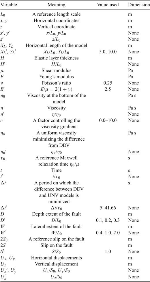
Variables used in this study.

Open in new tabDownload slide

2.1 Governing equations

We solve the equilibrium stress equation:

1

where is the stress tensor, ρ is the density and g_i is the gravity. We assume an isotropic elastic constitutive relationship between stress and strain, relaxed by viscous creep:

2

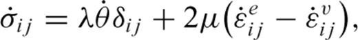
where λ and μ are the elastic constants (μ is the shear modulus), θ is the elastic dilatation and the superscripts e and v, respectively, indicate the elastic and viscous components of strain rate. The strain tensor is defined in terms of displacements u_i by

3

Viscous creep rate is related to the elastic strain by:

4

where η is the viscosity.

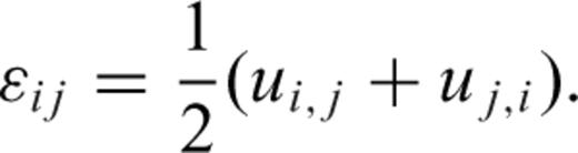
2.2 Finite element implementation

For the solutions of eqs (1)–(4), we use the parallelized finite element code, oregano_ve which solves the general Maxwell viscoelastic problem in a rectangular domain with arbitrary traction and displacement boundary conditions. We neglect body forces and assume linear viscous creep with a depth-dependent creep viscosity coefficient.

The fundamental equation in the finite element analysis (e.g. Hughes 2000) relates a displacement vector U to a load vector F operating on the nodes through an elastic stiffness matrix K over a domain Ω with boundary Γ: KU = F. Using a Galerkin formulation

5

where B relates nodal displacement to element strain, D is the elastic stiffness matrix that relates stress to strain and

6

where N is the shape function matrix, T is the applied traction vector at the boundary surface and ΔU_f is the prescribed displacement vector on the fault, which is implemented by means of the split node method developed by Melosh & Raefsky (1981). The model domain is discretized using tetrahedral elements (four vertex nodes and six midpoint nodes) with displacements described by quadratic interpolation functions.

An explicit time-stepping algorithm is used, following Zienkiewicz & Cormeau (1974) and Hughes & Taylor (1978). The increment of time is a fixed fraction of the Maxwell time constant: Δt_n = (η/μ)/24 (Cormeau 1975), using the minimum value of this ratio in the solution domain. The increment of viscous strain during the nth time step is:

7

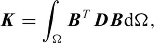
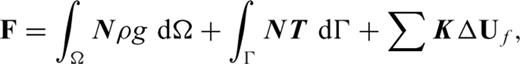
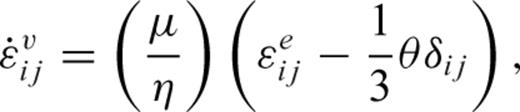
where is the viscous strain rate. The viscous displacement increment ΔU_n is obtained by solving the matrix equation:

8

Then the displacement and stress fields are updated by:

9

10

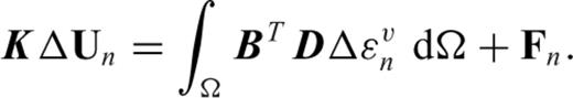
The oregano_ve code is parallelized by subdivision into similar layers, which are distributed to independent processors for assembly and solution of the matrix. Nodes are duplicated at processor interfaces. The main matrix equation is solved by the method of conjugate gradients. The accuracy of the oregano_ve code has been validated by comparison of numerical and analytic solutions (e.g. Yamasaki et al. 2010).

2.3 Geometry and boundary conditions for experiments

We define a dimensionless solution domain of unit thickness and widths in the horizontal directions of X′_L (=X_L/L₀) = 5.0, Y′_L (=Y_L/L₀) = 10.0, where L₀ is the scale length for distance, chosen here to be the layer depth. Displacements are scaled separately using the reference displacement S₀. The model domain comprises 300 000 tetrahedral elements (six elements packed in each cubic unit cell of length 0.1). In resolution tests co- and post-seismic total surface displacements, respectively, differ by less than ∼0.005 and ∼0.04 for unit-cell lengths between 0.1 and 0.05; the maximum difference was found at x′∼ 0.0, y′∼ 0.1, where Ux′∼ 0.65 and 0.77 for coseismic and post-seismic total displacements.

The following mechanical boundary conditions are adopted: zero displacement is specified on the base of the model (z′ = 1.0) and on all side boundaries. Zero traction is specified on the top surface (z′ = 0.0). The rigid lower boundary may be interpreted as the upper boundary of a more rigid mantle layer, or conceivably a more mafic lower crust. On the rectangular fault segment, a constant x-direction dimensionless displacement difference of 2 is imposed between the corresponding split nodes on either side of the fault within the slipped region of area (W×D). Outside the slipped region, the displacement difference is zero. Consistent with the discretized representation of the boxcar function, the displacement difference is 1 on the periphery of the slipped region. For simplicity, gravity is omitted from these calculations, in effect assuming that the lithostatic part of the stress field is a function of depth only and does not affect the deviatoric stress field. We implicitly assume that the density field is stratified and that any disturbance to the stratification produced by the strike-slip fault is negligible.

The viscosity model is effectively 1-D except for negligible effects caused by the side boundary conditions: The maximum change in the coseismic surface displacement caused by doubling X′_L and Y′_L for the reference calculation (W′ = W/L₀ = 1.0, D′ = D/L₀ = 0.2) is an increase of ∼0.0025 near x′ = 0.0, y′ = 0.1. After viscous relaxation has occurred, the maximum displacement change is an increase of ∼0.02 near x′ = 0.0, y′ = 2.0. Moving the side boundaries outward enables very minor viscoelastic adjustment to affect a larger volume. For the case of a larger fault (W′ = 2.0, D′ = 0.3), the same test showed respectively: ∼0.0012 and ∼0.048 for coseismic and total post-seismic displacement changes near x′ = 0.0, y′ = 2.0.

In all experiments, we set the depth extent of the fault (D′) equal to the thickness of the elastic layer, H′ (=H/L₀). We considered values of D′ = H′ = 0.1, 0.2 and 0.3 in our experiments. For the lateral extent of the fault (W′), we considered: W′ = 0.4, 1.0 and 2.0.

2.4 Viscosity structure

Viscous creep is generally described by a flow law, which includes an Arrhenius activation term (e.g. Kirby 1983; Poirier 1985). We simplify and approximate here to more efficiently explore the parameter space, and assume that the viscoelastic layer beneath the elastic layer has an exponential dependence of viscosity on depth:

11

where η₀ is the viscosity at the bottom of the model (z′ = 1), and c is a constant controlling the depth dependence.

In the elastic layer of thickness H′, we set viscosity η′ = 10²⁰. We use Poisson′s ratio ν= 0.25 and assume uniform elastic properties with dimensionless Young's modulus E′ = E/μ= 2(1 +ν) = 2.5, where μ is the shear modulus.

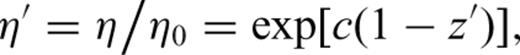
Viscosity versus depth for different values of c is depicted in Fig. 2. The base of the elastic layer is indicated by one of the horizontal dashed lines, so the sloping line is replaced by a constant value of 10²⁰ above this level. The ratio of viscosities between top and bottom of the viscoelastic layer is exp[c(1 –H′)]. We consider values of c between 0.0 (the UNV model) and 10.0.

Figure 2

The dependence of viscosity on depth for the viscoelastic model used in these calculations is controlled by the parameter c (eq. 11). The horizontal dashed lines indicate different values used here for the base of the elastic layer. Dimensionless viscosity is set to 10²⁰ above that level.

Open in new tabDownload slide

3 Results

3.1 General behaviour of UNV and DDV models

Fig. 3 shows upper surface displacement fields at three times for a UNV model with H′ = D′ = 0.2, W′ = 1.0, c = 0. Profiles of the surface displacement in x-direction (U′_x = U_x/S₀) along the lines x′ = 0.0, 0.5, 1.0 and 1.5 and the distributions of the surface displacements in x-, y- and z-directions (U′_x, U′_y = U_y/S₀ and U′_z = U_z/S₀) are depicted at times t′ (=t/τ₀, where τ₀ =η₀/μ) = 0.0, 8.33 and 41.66. Note that all displacements scale linearly with respect to S₀.

Figure 3

Variation of the surface displacements in x-, y- and z-directions (U′_x = U_x/S₀, U′_y = U_y/S₀ and U′_z = U_z/S₀) on the upper surface z′ = 0, at times t′ (=t/τ₀, where τ₀ is defined by η₀/μ) = 0.0, 8.33 and 41.66, for a constant viscosity layer beneath an elastic lid, with H′ = D′ = 0.2, and fault length W′ = 0.1. The top three graphs show profiles of U′_x along the lines z′ = 0.0, x′ = 0.0, 0.5, 1.0 and 1.5, at the same times.

Open in new tabDownload slide

The profiles of U′_x are antisymmetric with respect to the fault. As expected, the maximum U′_x is obtained on either side of the fault (y′ = 0.0) along the lines x′ = 0.0. For x′ = 1.0 and 1.5 (lines that are outside the lateral extent of the fault), U′_x = 0.0 at y′ = 0.0. For x′ = 0.5, (across the end of the fault), the maximum displacement is ±0.5, consistent with the discretized representation of the box-car slip function at the end of the fault.

The distributions of U′_x and U′_z at the surface are in general anti-symmetric with respect to the fault. U′_x decreases away from the fault on a length scale related to the length and depth extent of the fault. Significant U′_y is observed near the end of the fault, in a butterfly-like distribution, symmetric with respect to reflection in the fault. The distribution of U′_z is characterized by four localized displacement concentrations of alternating sign next to the ends of the fault, flanked by four broad regions where the displacements are small and of opposite sign to the adjacent displacement peak. The most obvious feature in the temporal evolution of U′_x, U′_y and U′_z is the increasing displacement amplitudes at intermediate distances, as viscous relaxation occurs. Note that Fig. 3 only shows the central part of the upper surface; the far-field displacements approach zero as the side boundaries are approached.

Fig. 4 shows displacement fields for a DDV model with c = 5.0 and other parameters as in Fig. 3 (H′ = D′ = 0.2 and W′ = 1.0). The distributions of U′_x, U′_y and U′_z in UNV and DDV models are similar (compare Figs 3 and 4), but the viscoelastic relaxation occurs more slowly for c = 5.0 because the viscosity at the top of the viscous layer is increased by a factor of ∼100. The most obvious differences occur in the U′_z distribution, where the long-term displacements at intermediate distances, though small in both models, are evidently greater in the DDV model. This difference is compensated to some extent by smaller DDV long-term displacements in U′_x and U′_y in the same distance ranges. Comparable observations of a DDV model have been described by Riva & Govers (2009).

Figure 4

Variation of the displacements, U′_x, U′_y and U′_z, at t′ = 0.0, 8.33 and 41.66, on the upper surface, z′ = 0 for depth-dependent viscosity with c = 5.0 and fault configuration specified by D′ = H′ = 0.2 and W′ = 1.0. The top three graphs show profiles of U′_x along the lines z′ = 0, x′ = 0.0, 0.5, 1.0 and 1.5, at the same times.

Open in new tabDownload slide

The impact of fault length on the distribution of U′_x in the y–z plane (x′ = 0.0) at t′ = 0.0, 8.33 and 41.66 is shown in Fig. 5 for the DDV model with W′ = 0.4, 1.0 and 2.0 (Figs 5a–c). Other parameters are as in Fig. 4 (c = 5.0 and D′ = H′ = 0.2). At t′ = 0.0, U′_x is mainly distributed within the elastic layer whose base is indicated by the horizontal dashed line. In the post-seismic period, strain progressively diffuses into the viscoelastic layer beneath. In general, the volume of rock affected by the fault slip increases with W′ (most clearly for t′ = 41.66 in Fig. 5). We have found that the half width of the displacement profile scales approximately as W′^1/2.

Figure 5

Variation of displacement U′_x on the y–z plane (x′ = 0.0) at times t′ = 0.0, 8.33 and 41.66, for depth-dependent viscosity calculations with c = 5.0, D′ = H′ = 0.2 and fault lengths: (a) W′= 0.4, (b) W′= 1.0 and (c) W′= 2.0. Contour interval is 0.2.

Open in new tabDownload slide

Fig. 6 shows post-seismic displacement U′_x(t) –U′_x(0) profiles along x′ = 0.0 at t′ = 41.66 for different fault configuration and viscosity structure. The maximum post-seismic displacement is obtained at distances from the fault of ∼0.3–0.5, the peak occurring further out for greater D′, W′ and c. The amplitude of post-seismic displacements appears to decrease strongly with c, but actually the timescale for relaxation is increasing with the near-surface viscosity; if there is time for complete relaxation, the same final displacement is expected.

Figure 6

The post-seismic component of displacement U′_x along the line x′ = 0.0 for fault lengths: (a), (d) and (g) W′ = 0.4, (b), (e) and (h) W′ = 1.0 and (c), (f) and (i) W′ = 2.0. Depth extent of faults: (a), (b) and (c) D′ = H′ = 0.1, (d), (e) and (f) D′ = H′ = 0.2 and (g), (h) and (i) D′ = H′ = 0.3. In each case c = 0.0, 2.0, 5.0 and 8.0.

Open in new tabDownload slide

Fig. 7 shows, for different viscosity structures, the time-dependence of U′_x at two surface points distant 0.1 and 1.0, respectively from the centre of the fault (for D′ = H′ = 0.2 and W′ = 1.0 as in Fig. 4). The black and grey (dashed) curves, respectively, show the behaviours of DDV and UNV models. We show surface displacements of UNV models for values of η′ between 1.0 and 100.0. For DDV models, we show displacements for c = 0.5, 1.0, 2.0, 3.0, 4.0, 5.0, 6.0, 8.0 and 10.0. Note that the UNV solutions at a given location are mathematically identical; the timescale is simply stretched in proportion to η′.

Figure 7

The time dependence of U′_x at two points on the upper surface: (a) (x′, y′, z′) = (0.0, 0.1, 0.0) and (b) (x′, y′, z′) = (0.0, 1.0, 0.0) for different viscosity structures. The black and grey (dashed) curves indicate DDV and UNV models, respectively, with viscosity parameters as labelled and other parameters: H′ = D′ = 0.2 and W′ = 1.0.

Open in new tabDownload slide

Near the fault (Fig. 7a), at (x′, y′, z′) = (0.0, 0.1, 0.0), the initial elastic displacement (U′_x = 0.6528) is a relatively large fraction of the final displacement (Figs 3 and 4). As the viscous relaxation progresses, U′_x at this point increases asymptotically to a value of approximately 0.7775. Thus the component of U′_x because of the viscous relaxation is 0.1247. The time to reach the convergence value increases in direct proportion to η′; for a UNV model with η′ = 1.0, U′_x is ∼99.35 per cent converged at t′ = 40. The surface displacement rates, therefore, are strongly dependent on the viscosity structure; faster rates are obtained for models with lower average viscosity.

Fig. 7 also shows that the behaviour of a DDV model with c > 0 is similar to that of a UNV model for some η′ > 1 at each location. For example, the UNV model with η′ = 5.0 at y′ = 0.1 shows a displacement history that falls between those of the DDV models with c = 2.0 and 3.0 and the UNV model with η′ = 50.0 is similar to a DDV model with c∼ 7. We may associate an apparent viscosity with a depth in the DDV model by inverting eq. (11):

12

so we may summarize this comparison by stating that the DDV model at this location behaves approximately like a UNV model whose viscosity is equal to the DDV viscosity at z′∼0.45. If we consider c-values between 0 and 10, the implied depth may vary by ∼±10 per cent.

Further from the fault (Fig. 7b), at (x;, y;, z;) = (0.0, 1.0, 0.0), the initial elastic displacement (U′_x = 0.0197) is a relatively small component of the eventual converged displacement (∼0.0962), and the component of U′_x because of viscous relaxation is ∼0.0765 at this location. Fig. 7(b) also shows that, whereas the DDV displacement history at this location can be well approximated by a UNV model if c is less than about 1, the histories of DDV models with c > 1.0 show a significant decrease in rate of displacement during relaxation which cannot be precisely matched by any UNV model. This difference increases with c. Whether such small differences in displacement history could be measured in practice, however, is questionable.

3.2 Difference between UNV and DDV models

3.2.1 Comparison of UNV and DDV models at specific surface points

To further quantify this comparison between predictions of UNV and DDV models, we show in Fig. 8 the time-dependent U′_x at four specific surface points on the y′ axis: (x′ = 0.0, z′ = 0.0), y′ = 0.1, 0.2, 0.5 and 1.0. Displacement histories of DDV models with c = 2.0, 5.0 and 8.0 are depicted in Figs 8(a), (b) and (c), respectively, for D′ = H′ = 0.2 and W′ = 1.0. In each case, we also plot the time history for a UNV model for which the layer viscosity η_u' is chosen to minimize the difference between UNV and DDV model displacements at that point. We make a simple 1-D grid search to find the best-fit UNV model using an increment of 0.01 in dimensionless UNV viscosity. The best-fit UNV viscosity depends weakly on the time interval examined. In Fig. 8, we used a fixed time-period Δt′ = 41.66 (1000 time steps). Later we consider the impact of changing that time interval.

Figure 8

Displacement histories U′_x (t′) at four surface points: (x′, y′, z′) = (0.0, 0.1, 0.0), (0.0, 0.2, 0.0), (0.0, 0.5, 0.0) and (0.0, 1.0, 0.0) for different viscosity models. The black and grey (dashed) curves indicate DDV and UNV models, respectively. For DDV models: (a) c = 8.0, (b) c = 5.0 and (c) c = 2.0. The UNV model shown in each case uses the dimensionless viscosity value η_u′ which provides the best fit to the DDV displacement history on a time period of Δt′ = 41.66 at that point. In each case H′ = D′ = 0.2 and W′ = 1.0.

Open in new tabDownload slide

The rate of displacement increase for the DDV model is respectively greater and smaller than that of the best-fit UNV model in earlier and later phases, for all values of c, though the displacements are almost linear with time for the larger values of c, because the time span examined in Fig. 8 is still in the early (unrelaxed) phase of viscoelastic relaxation. However, the difference between the two models depends on the distance from the fault. In the near field, and for small c, a UNV model can be found that closely fits the DDV model (Fig. 8, upper left). On the other hand, at greater distances from the fault, or for large c (Fig. 8, lower right), the differences between UNV and DDV models are greater; the DDV model behaves as if its apparent viscosity increases with time.

Acknowledging that such differences may be significant, we show in Fig. 9, the apparent UNV (η_u′) which best fits the DDV model displacement history on a time period Δt′ = 41.66 at different locations (x′, y′), relative to the fault. The estimates of η_u′ for DDV models with c = 8.0, 5.0 and 2.0 are shown in Figs 9(a), (b) and (c), respectively (with D′ = H′ = 0.2 and W′ = 1.0). From these graphs, it is apparent that the value of η_u′ that best represents a DDV model generally decreases with distance from the fault, at a rate that depends on the viscosity gradient c. For the DDV model with c = 8.0, η_u′ decreases by a factor of about 10, from ∼87 at y′ = 0.1 to ∼8 at y′ = 1.0. For c = 5.0, η_u′ decreases from ∼23 at y′ = 0.1 to ∼5 at y′ = 1.0. For c = 2.0, η_u′ decreases from ∼3.7 to ∼2.4 in the same distance range. For y′ > 1.0, displacements are small but the apparent viscosity generally changes little with further distance from the fault and, typically, an apparent viscosity close to the DDV viscosity at mid-depth would be inferred (z′ between 0.35 and 0.55).

Figure 9

The UNV model viscosity η_u′ which best fits a given DDV model displacement history on a time period Δt′ = 41.66 is here plotted as a function of distance from the fault for: (a) c = 8.0, (b) c = 5.0 and (c) c = 2.0. The filled circle, open circle and filled square show values determined at points on the lines x′ = 0.0, ±0.5 and ±1.0, respectively. In each case H′ = D′ = 0.2 and W′ = 1.0.

Open in new tabDownload slide

Similar changes in η_u′ with distance from the fault plane are evident along y-direction lines offset from the fault centre. On the perpendicular line from the end of the fault, the apparent viscosity is increased by perhaps 50 or 100 per cent compared to x′ = 0 (Fig. 9; x′ =±0.5). Beyond the end of the fault (Fig. 9; x′ =±1.0), the apparent viscosity may be as much as two or three times greater than that determined on the y′ axis. Note, however, that the post-seismic displacements at such distances from the fault are small relative to the expected measurement noise so this type of interpretation may only be practical in near-fault regions (x′ < ±W′/2, y′ < ±1.0).

We note here that the best-fitting η_u′ for a given c-value at each surface point depends on the time period Δt′ on which the difference between the two models is minimized. However, changes to the graphs shown in Fig. 9 are small.

3.2.2 Dependence on the fault configuration

The apparent viscosity η_u′ also depends on the parameters describing the fault configuration: the depth extent D′, here assumed equal to the thickness of the elastic layer, H′, and the lateral extent, W′. Similar to Fig. 9, we show in Fig. 10, the viscosity η_u′ of the UNV model which best fits the DDV model displacement history on the time period Δt′ = 41.66 at the same set of surface locations. In these calculations, D′ = H′ = 0.1 (Fig. 10a) or 0.3 (Fig. 10b) and again W′ = 1.0. The dependences of η_u′ on distance from the fault and on the viscosity gradient are similar in Figs 9 and 10: close to the fault, η_u′ is greatest (∼240 for D′ = 0.1 and c = 8.0), but the peak value decreases with increasing D′. The rate of decrease of the apparent viscosity with distance from the fault is also reduced for greater D′. Near the fault, the dependence of η_u′ on D′ in these experiments is broadly consistent with the idea that the response is dominated by viscosities at depths between about 0.1 and 0.25 (at y′ = 0.1), 0.14 and 0.27 (at y′ = 0.2), 0.27 and 0.44 (at y′ = 0.5), 0.33 and 0.66 (at y′ = 1.0), 0.29 and 0.77 (at y′ = 1.5), 0.20 and 0.86 (at y′ = 2.0), below the base of the elastic layer. For larger D′, the system sees lower viscosities because relatively high viscosity shallow material has been replaced by a thickened elastic lid. At large y′, however, η_u′ is almost independent of D′, presumably because the long wavelength deformations required for far-field adjustment are in each case mediated by the relatively lower viscosities below z′∼0.3.

Figure 10

The UNV model viscosity η_u′ which best fits a given DDV model displacement history on a time period Δt′ = 41.66 is here plotted as a function of distance from the fault for elastic layer thickness (= depth of fault): (a) D′ = H′ = 0.1 and (b) D′ = H′ = 0.3, for viscosity gradients: (i) c = 8.0, (ii) c = 5.0 and (iii) c = 2.0. The filled circle, open circle and filled square show values determined at points on the lines x′ = 0.0, ±0.5 and ±1.0, respectively. In each case W′ = 1.0.

Open in new tabDownload slide

The difference between DDV and optimum UNV model displacements is shown for different values of the fault depth extent, D′, at four specific surface points: (x′ = 0.0; y′ = 0.1, 0.2, 0.5, 1.0; z′ = 0.0) in Figs 11(a)–(d), assuming c = 8.0 and W′ = 1.0. The difference, U_{x_DDV}′−U_{x_UNV}′, shown in Fig. 11 indicates a greater displacement in the DDV model than in the UNV model for model times less than about t′ = 30, and lesser displacement thereafter. The maximum difference increases generally with distance from the fault y′, with fault depth extent D′ and (after t′∼30) with further elapsed time. Fig. 12 shows that the difference between DDV model and best-fit UNV model is approximately doubled when W′ is doubled (for D′ = H′ = 0.2 and c = 8.0).

Figure 11

The difference in displacement: U_{x_DDV}′–U_{x_UNV}′, as a function of time at four surface points on the y′ axis (x′ = 0, z′ = 0): (a) y′ = 0.1, (b) y′ = 0.2, (c) y′ = 0.5, and (d) y′ = 1.0 and three different values of the elastic layer thickness (= fault depth): D′ = H′ = 0.3, 0.2 and 0.1. In each case the UNV model viscosity η_u′ is chosen to best fit the DDV model displacement history on a time period Δt′ = 41.66 at that point. For these calculations, c = 8.0 and W′ = 1.0.

Open in new tabDownload slide

Figure 12

The difference in displacement: U_{x_DDV}′–U_{x_UNV}′, as a function of time at four surface points on the y′ axis (x′ = 0, z′ = 0): (a) y′ = 0.1, (b) y′ = 0.2, (c) y′ = 0.5 and (d) y′ = 1.0 and three different values of the fault length W′ = 0.4, 1.0 and 2.0. In each case the UNV model viscosity η_u′ is chosen to best fit the DDV model displacement history on a time period Δt′ = 41.66 at that point. For these calculations, c = 8.0 and H′ = D′ = 0.2.

Open in new tabDownload slide

Fig. 13 shows that the variation of best-fit UNV viscosity η_u′ with distance from the fault is not strongly affected by increasing W′ from 1 to 2, with D′ = H′ = 0.2 and c = 2.0, 5.0 and 8.0. The total variation of η_u′ seen in Fig. 9 is preserved, to a good approximation but the rate at which η_u′ decreases away from the fault is reduced by a small factor.

Figure 13

The UNV model viscosity η_u' which best fits a given DDV model displacement history on a time period Δt' = 41.66 is here plotted as a function of distance from the fault for: (a) c = 8.0, (b) c = 5.0 and (c) c = 2.0. In each case H' = D' = 0.2. The black and grey curves indicate values determined for W' = 2.0 and 1.0, respectively. Filled circles show values determined on the lines x' = 0.0 (across the centre of the fault) and open circles show values on lines perpendicular to the end of the fault, (x' =±0.5 or ±1.0, for W' = 1.0 or 2.0, respectively).

Open in new tabDownload slide

In Fig. 14, we summarize how the decrease in η_u′ with distance from the fault depends on the parameter values of c, D′ and W′. For each of the x′ = 0.0 lines on Figs 9, 10 and 13, we calculated a best-fit line to the graph of log(η_u′) versus y′. We used only those parts of the line near the fault which showed an approximately linear variation (y′≤1.0), and we show the slope and the intercept of each line on Figs 14(a) and (b), respectively, as a function of viscosity gradient c. In addition, we also examined the sensitivities of the slope and the intercept to the time period Δt′ for which the best-fit UNV model is obtained. The upper and lower limits of the error bars on Fig. 14 are obtained for Δt′ = 41.66 and 5, respectively. We confirmed also that the measurements of slope and intercept are not significantly changed for Δt′ > 41.66, implying that the viscosity gradient can be sufficiently estimated by focussing on the early post-seismic phase.

Figure 14

The slope (a) and the log(intercept) (b) of the best-fit line from the x' = 0 graphs of log(η_u') versus y' on Figs 9, 10 and 13 shown here as a function of c. Best-fit lines are determined using only the linearly varying data near the fault (y'≤ 1.0). Results are shown for H' = D' = 0.1, 0.2 and 0.3 and W' = 1.0 and 2.0. Upper and lower limits on the error bars show the slope and log(intercept) evaluated for observational time periods of Δt' = 41.66 and 5, respectively; the plotted point shows the average of the two values.

Open in new tabDownload slide

Both slope and intercept linearly increase in magnitude with c, but the linear dependence is affected by D′. For the same value of c, the slope is approximately doubled in magnitude when D′ is changed from 0.3 to 0.1. The slope decreases in magnitude as W′ is increased. Although the intercept of the best-fit line varies inversely with D′ (because the maximum η′ in the viscoelastic layer is greater for smaller D′), it is insensitive to W′. The intercept is insensitive to Δt′. However, the slope has a weak dependence on Δt′ for models with W′ = 1.0 and D′ = 0.1 and 0.2. Minor uncertainty in the value of c (∼1.4) inferred from a measured slope could arise if Δt′ is poorly chosen.

In all these examples, our analysis shows that, although the difference relative to a UNV model may well be practically undetectable at any given measurement point, the systematic decrease in apparent η_u′ with distance from the fault should be measurable even for small values of the vertical viscosity gradient c. Moreover, the total viscosity contrast and the rate at which it decreases away from the fault are, in principle, diagnostic of the vertical viscosity gradient and the fault dimensions.

4 Factors Controlling the Viscous Relaxation in Post-Seismic Deformation

Deformation of the lithosphere is the product of an interaction between the driving force (loading/unloading) and the rheology of the constituent rocks. In the Maxwell viscoelastic problem, elastic stress developed in the viscoelastic layer by fault slip drives the subsequent viscous relaxation. For a given magnitude of elastic stress, the relaxation rate is primarily controlled by the viscosity of the stressed ductile layers; the rate of stress relaxation is inversely related to the Maxwell relaxation time defined by η/μ, where η is the viscosity and μ is the shear modulus. In the general DDV problem, both the magnitude of deviatoric stress and the viscosity are spatially variable: in general, stress magnitude decreases with distance from the fault, and creep viscosity decreases with depth. In the near field, fault slip introduces relatively large-magnitude elastic stresses at relatively shallow depths, so that the relaxation of these stresses is mainly governed by the higher viscosity rocks at shallow depths. Deformation of the far field, however, requires viscous relaxation at greater depths, where the viscosity is less. Thus we see apparently lower viscosities at observation points further removed from the fault.

For the problem of post-seismic viscous relaxation in a Maxwell medium in which creep viscosity depends on depth only, we have shown that, in general, the displacement history at any specific place on the surface approximately follows the history that would be predicted for a UNV model, for appropriately chosen viscosity η_u. Although the quality of this fit decreases with distance from the fault for large viscosity gradients, c (Fig. 8), we have established that the variation of the apparent η_u with distance from the fault is a reliable measure which is sensitive to the rate at which creep viscosity decreases with depth in the crust (Figs 9, 10, 13 and 14).

For this type of 1-D viscosity variation we have shown empirically that the logarithm of the apparent creep viscosity η_u decreases almost linearly (i.e. the apparent creep viscosity η_u decreases almost exponentially) with distance from the fault for distances within about one-layer depth (y′ < ∼1.0). Approaching the fault, η_u increases rapidly to peak values that are representative of viscosities in the depth range 0.1 to 0.25 below the base of the elastic lid (Figs 9 and 10). At greater distances, the model η_u values are relatively constant for a given value of the viscosity-depth coefficient c, and generally are consistent with the model viscosity at depths between 0.65 and 0.75 below the upper surface. This far-field apparent viscosity does not depend strongly either on the fault depth extent D′, or on the fault length, W′; equilibration of stress on the longer wavelengths simply depends on the bulk viscosity of the layer at median depths. However, we note here that displacements at these distances (y′ > ∼1.0) are sufficiently small that reliable measurements of the post-seismic relaxation phase are unlikely to be obtained.

The near-field viscoelastic relaxation is clearly dominated by the higher stresses developed at shallow depths below the slipped fault. As these near-field stresses gradually relax, they remain always the dominant element in the stress-relaxation observed near the fault. Thus, the DDV model displacement history in the near field closely resembles that predicted by a UNV model. In contrast, we see the greatest deviations from UNV behaviour in the far field, where the early displacements are in response to relatively low stresses in the relatively low-viscosity mid-layer region, and the later displacements are slowed by relaxation in the somewhat greater viscosities at shallower depths. These differences of course increase with the viscosity gradient, c (Fig. 8).

We also find that the difference between DDV and best-fit UNV models, whereas remaining relatively small in an absolute sense, increases almost in proportion to D′ (Fig. 11) and W′ (Fig. 12). We have shown that the depth extent of the faulted elastic layer influences the post-seismic viscous relaxation in so far as the apparent near-field viscosity η_u decreases with greater fault depth extent (Figs 10 and 14). This observation is simply consistent with the increase in thickness of the elastic layer requiring that the viscosity at the top of the viscoelastic layer is reduced in our model (Fig. 2). In each case, we find that the apparent near-field viscosity falls within the range of DDV viscosity at depths between 0.12 and 0.25 below the elastic lid. As fault depth increases, the elastic stresses are distributed to a greater volume beneath the fault. The increased range of viscosities that affect the solution therefore enhances the difference between the DDV model and the optimum UNV model.

Although the volume affected by fault slip increases significantly with fault length W′ (Fig. 5), W′ seems to have relatively minor effect on the relationship between η_u and distance from the fault (Fig. 13), presumably because the viscosity structure is insensitive to W′.

5 Discussion

Coseismic displacements of the region surrounding a fault can be used to evaluate the slip distribution on the fault by matching the elastic model prediction to geodetic observations (e.g. Suito & Hirahara 1999; Reilinger et al. 2000; Pritchard et al. 2002; Pollitz et al. 2005; Funning et al. 2007). Such studies provide important constraints on the redistribution of elastic stress that accompanies an earthquake. This stress field also is the basis for any computation of the post-seismic viscous relaxation.

Many previous studies have revealed that the univiscous Maxwell viscoelastic model does not explain an apparent increase in viscosity observed in later phases of relaxation at fixed observation points (e.g. Pollitz 2003, 2005; Freed & Bürgmann 2004; Ryder et al. 2007; Hearn et al. 2009). Alternative transient rheology models have been proposed to explain this increase, including the standard linear solid (e.g. Hetland & Hager 2005; Ryder et al. 2007), the biviscous Burgers model (e.g. Pollitz 2003, 2005; Hetland & Hager 2005, 2006; Hearn et al. 2009), the triviscous viscoelastic model (e.g. Hetland & Hager 2005) and the power-law rheology model (e.g. Freed & Bürgmann 2004).

If the decrease of viscosity with depth is taken into account, however, the linear Maxwell model also predicts an apparent increase in viscosity with time at any given location (as found by Riva & Govers 2009). More importantly, the depth dependence of viscosity is revealed in large variations of apparent viscosity with distance from the fault. Our analysis, based on determination of an equivalent UNV viscosity, suggests a simple procedure for the analysis of a geodetic data set that constrains post-seismic relaxation: for a given fault configuration (D, W and S) obtained from coseismic deformation, (1) at each of several observation points determine the apparent (best fit) viscosity based on a UNV model, (2) plot the log(η_u) values versus distance, to determine the slope, (3) interpret a c-value from Fig. 14 and (4) determine the reference viscosity η₀, by scaling the prediction of the relevant DDV model to obtain a best-fit match to the temporal evolution of the surface displacement at all measurement points.

The boundary conditions and viscosity structure adopted in this study have a simple physical interpretation consistent with standard rheological models of the Earth in which the uppermost mantle has a relatively high strength beneath a crust in which strength systematically decreases with depth because of increasing temperature. Variation of the chemical composition with depth (e.g. Jackson 2002; Burov & Watts 2006), however, could cause a more complex stratification of the viscosity profile (Riva & Govers 2009), which would require further investigation using, for example multilayer models of the crust.

The determination of the viscosity law which best describes post-seismic relaxation needs to follow a systematic procedure whose aim is to find the simplest physically justifiable model which can fit available data. We restrict ourselves here to a linear Maxwell viscoelastic law to evaluate the first-order effect of depth-dependent temperature on post-seismic viscous relaxation. Although crustal materials also exhibit a stress-dependent viscosity, we omit that further complexity here. We can argue that, although the material may be non-linear, its response in the post-seismic situation may be approximately linear if the stress perturbation caused by the earthquake is generally small relative to the prevailing background deviatoric stress. Therefore, we should test first whether a stratified linear viscosity model can explain the available data, and use that test to determine if a more complex model is needed.

The spatial dependence of post-seismic displacements has previously been suggested as a discriminant of relaxation mechanism. Freed et al. (2006b) showed that the post-seismic deformation following the 2002 Denali (Alaska) earthquake cannot simply be explained by viscoelastic relaxation; afterslip is also clearly implicated. Hearn et al. (2009) reached a similar conclusion for the post-seismic deformation of the 1999 Izmit-Düzce (Turkey) earthquake. Ryder et al. (2007) concluded that the surface deformation following the 1997 Manyi (Tibet) earthquake observed from the InSAR data can be explained by either viscous relaxation or afterslip, and it is difficult to separate the one from the other.

Viscoelastic relaxation following an earthquake, has a rather well-defined behavior characterized by a length scale which is primarily determined by the geometry of the fault break, and a timescale which is primarily determined by the viscosity profile of the ductile layer beneath. If the signature of afterslip has distinctly different length or timescale, then it should be possible to separate the signatures of the two processes. Clearly, however, this separation of the signals from different processes is only feasible if the geodetic data set provides a clear determination of the spatial and temporal dependences of post-seismic ground displacement.

6 Conclusions

In this study, using 3-D finite element calculations, we have examined the effect of a DDV structure on the linear Maxwell viscoelastic response to an instantaneous strike-slip fault event. We have shown that the ground displacement histories predicted from DDV models compare closely to those predicted from UNV models, but the equivalent UNV varies with position relative to the fault.

We find that the apparent viscosity (η_u) determined at different locations above a DDV model decreases with distance from the fault, and the rate of decrease of η_u with distance increases with the DDV viscosity gradient (Fig. 14). Near the fault, the DDV model behaviour at an individual observation point can be well reproduced by a UNV model. In the far field, however, the DDV model displacement histories show rates of change that are characterized by viscosity apparently increasing with time. Our analysis suggests a practical procedure for analysing a geodetic data set for the key parameters that define a DDV model of post-seismic viscoelastic relaxation: viscous layer thickness, reference viscosity and viscosity gradient, assuming that fault-geometry parameters are already established.

The linear Maxwell DDV model described in this study requires further testing against geodetic data sets, which constrain the spatial and temporal variation of ground displacement following an earthquake. Of course, valid arguments may be made as to why other more complex rheological models representing for example, laterally varying viscosity, non-Newtonian viscosity or transient rheology should be used. Before accepting the requirement for more complex rheological models, however, we should first establish whether a simple stratified Maxwell viscoelastic model can explain a geodetic data set and, if not, why not.

Acknowledgments

We thank Tim J. Wright for stimulating discussions and valuable suggestions. This study is supported by the UK Natural Environment Research Council (NERC) under the program of the National Centre for Earth Observation (NCEO-COMET+). Original development work on oregano_ve was carried out by Elek Postek, with the support of EPSRC and the collaboration of Peter Jimack. Cluster computing was provided by NCEO and by the University of Leeds Advanced Research Computing Node 1 (arc 1). Constructive reviews by two anonymous reviewers have significantly improved the manuscript.

References