Deformation of an elastic shell with variable thickness: a comparison of different methods

Summary

1 Introduction

The topographic load at the surface of a planet or a moon causes pressure variations that must be counterbalanced by static and/or dynamic forces of internal origin. The nature of these forces depends on the rheological properties of the body and, consequently, on its material composition and thermal state. In the absence of seismic data, gravity and topography are often the only observations available to geophysicists that can be used to constrain the deep structure and material properties of solar system bodies.

Topography is usually supported by a combination of three basic physical mechanisms: isostasy, viscous flow driven by density heterogeneity inside the body, and deformation of the uppermost elastic layer in response to surface loading. The analysis of topographic information in conjunction with gravitational data (if available) can indicate which of the mechanisms is dominant and thus helps in understanding the physical state of the body's interior (e.g. McKenzie et al. 2002; Roberts & Zhong 2004; Pauer et al. 2006).

In this paper, we focus on the elastic deformation of an outer shell (elastic lithosphere) of a planetary body due to surface and internal loading. The concept of an elastic lithosphere is based on the assumption that the outer layer behaves as an elastic solid, that is, it can maintain stresses induced by surface deformation over very long timescales. Therefore, the viscosity of this layer has to be sufficiently high for viscous relaxation to be negligible, and simultaneously the stresses have to be small enough not to induce fracturing and low temperature creep. At present, such conditions are likely to be satisfied on some one-plate planets with sufficiently thick upper thermal boundary layers, such as Mars or Mercury, and also on some silicate and icy moons (for discussion of effective elastic thickness, see, e.g. Burov & Diament 1995; Grott & Breuer 2008; Golle et al. 2012).

The response of the elastic lithosphere to surface loading depends on the thickness of the layer and its elastic parameters. Assuming the thickness of the shell to be uniform and small in comparison with the shell radius, Turcotte et al. (1981) derived an analytical expression for the thin shell response. This has found wide applications in planetology and is still one of the basic tools used in studying the internal dynamics of terrestrial bodies and some icy satellites (e.g. Lowry & Zhong 2003; Pauer et al. 2006; Nimmo et al. 2011). On Mars, the formalism developed by Turcotte et al. (1981) has been used not only to evaluate the lithospheric deflection and gravitational signal induced by topographic loads (e.g. Turcotte et al. 2002; McGovern et al. 2002; Belleguic et al. 2005; Beuthe et al. 2012) but also to estimate the possible deformation of the surface due to mantle convection (Zhong 2002; Roberts & Zhong 2004).

The method of Turcotte et al. (1981) is strictly valid only for a thin shell of constant thickness. However, a number of studies dealing with convective cooling of planetary bodies suggest that, at a given time, the elastic lithosphere thickness can show significant lateral variations (e.g. Solomon & Head 1990; Anderson & Smrekar 2006; Grott & Breuer 2010; Orth & Solomatov 2011). A thin shell approximation suitable for this case has been derived by Beuthe (2008) who showed that, under certain assumptions, the problem can be formulated in terms of a coupled system of linear fourth-order partial differential equations. Although the numerical solution of this problem is more demanding than in the case of an elastic shell of uniform thickness, it remains computationally feasible due to the 2-D nature of the thin shell approximation. It should be noted, however, that the accuracy of both approaches is limited and decreases with increasing shell thickness and decreasing wavelength of the load.

In this paper, we compare the thin shell approximations by Turcotte et al. (1981) and Beuthe (2008) with the spectral and finite element calculations obtained for a shell of finite thickness. The goal of this comparison is (i) to evaluate the error of both thin shell approximations, (ii) to assess the effect of shell-thickness variations on local deformation and, possibly, (iii) to provide benchmark results for the community dealing with the flexural response of an elastic lithosphere. In addition, we discuss whether the constant thickness approximation of Turcotte et al. (1981) can be used to estimate the deformation of a shell of variable thickness and whether the approach of Zhong (2002) can be generalized accordingly.

When discussing variations of elastic lithosphere thickness, we must distinguish between the real variations of the lithosphere thickness, existing at a given time and resulting from the instantaneous thermal and stress state of the planet, and the variations that are obtained from analysis of topography and gravity data and that may represent the thickness of the elastic lithosphere in different times in the past (e.g. McGovern et al. 2002). In this paper, we only deal with the former type of the elastic thickness variations and we do not address the problem of ‘frozen-in’ deformation (e.g. Courtney & Beaumont 1983; Albert & Phillips 2000).

The structure of the paper is as follows. In Section 2, we formulate the problem of elastic shell deformation and describe various approaches to its solution (thin shell approximation, spectral method, finite element methods). In Section 3, we discuss the assumptions and estimate the limitations of the thin shell approach. In Section 4, we compare all computational approaches in the case of uniform and variable shell thickness, and we discuss the influence of these variations on local deformation in more detail in Section 5. Section 6 deals with an extension of the approach of Zhong (2002) for a variable lithospheric thickness. All results are summarized and discussed in Section 7.

2 Governing Equations and Methods of Solution

2.1 Formulation of the problem

We consider an isotropic linearly elastic spherical shell deformed by a topographic load imposed at the surface. The elastic properties of the shell are represented by Young's modulus E and Poisson's ratio ν which are assumed to be constant. The density of the shell is ρ_c in the upper (crustal) part and ρ_m in the bottom (mantle) part, with the interface being located at depth t_c. For simplicity, we neglect the changes in density due to volumetric deformation as well as the effect of self-gravitation, and we assume that the bottom boundary of the shell is stress-free. Considering only static equilibrium, deformation of the shell is governed by the following equations:

1

2

with the boundary conditions

3

4

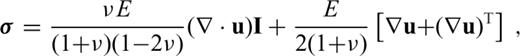
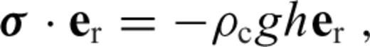
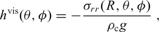
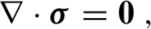
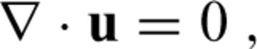
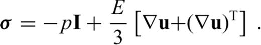
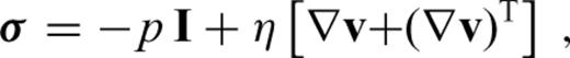
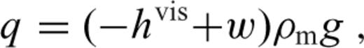
prescribed at the surface and the bottom boundary, respectively. Here, is the stress tensor, u is the displacement with w denoting its radial component, e_r is the unit radial vector, g is the gravitational acceleration, δ is the Dirac delta-function, r is the radius, R is the radius of the surface, I is the identity tensor, •^T denotes transposition of a matrix, and h is the topographic height.

In Sections 3–5, we will discuss the solution of the above problem for two end-member cases corresponding to t_c→ 0 and t_c→d where d is the thickness of the shell. In both of these cases the second (buoyancy) term in eq. (1) vanishes and is replaced by an equivalent force contribution in the boundary conditions. Namely for t_c→ 0, eq. (3) takes the form

5

while, for t_c→d, the condition at the bottom boundary (eq. 4) becomes

6

The resultant radial displacement can be used to compute the geoid which is a superposition of the gravitational signals induced by the surface topography and the mass anomalies arising from the deflection of the density interface inside the shell. Using the fully normalized spherical harmonics {Y_ℓm} as the basis functions (for definition, see Edmonds 1974; Jones 1985; Varshalovich et al. 1988), the geoid height can be expressed as follows:

7

where

8

Here, ℓ and m denote the degree and order of a spherical harmonic function, ℓ_max is the cut-off degree, G is the gravitational constant and h_ℓm and w_ℓm are the coefficients in the spherical harmonic series of topography h and radial displacement w, respectively. In the following, we will suppress the order subscript m in the cases where the general behaviour of functions H, h and w depends only on the degree ℓ.

2.2 Thin shell approximation

In a number of geophysical applications, the thickness of the elastic shell is significantly smaller than its radius. This property allows the original 3-D problem to be reduced to its effectively 2-D (thin-shell) approximation. A great variety of such approximations have been devised under different physical assumptions in many branches of science and technology. For linearly elastic materials, these include the classical Love-Kirchhoff (1st order) thin-plate theory, theories of second and higher orders (e.g. Vlasov 1949), their further generalizations obtained by including the transverse shear stresses (e.g. Reissner 1952; Naghdi 1957), and many others, see, for example, Kraus (1967) or Venstel & Krauthammer (2001) for a comprehensive review. In planetology the first-order thin-plate theory was used by Turcotte et al. (1981) who derived a spectral solution for a thin elastic shell of constant thickness (hereinafter referred to as TSA-T). In the following, we will use the relationship between the spherical harmonic expansion coefficients of topography h_ℓm and radial displacement w_ℓm derived by Turcotte et al. (1981) and modified by Willemann & Turcotte (1982):

9

where C_ℓ is the degree ℓ compensation coefficient,

10

with τ and σ defined as follows

11

12

The value of the coefficient C_ℓ ranges between 0 and 1, with the two end-members corresponding to an infinitely stiff elastic shell and a purely isostatic case, respectively. For the sake of consistency with other computational methods used in our study, we neglect the effect of self-gravitation included in the original formalism. In practice this means that the topographic height in eq. (9) is related to the sphere of radius R and not to the geoid (cf. eqs 4 and 21 in Turcotte et al. 1981).

The thin shell approximation (9) is strictly valid only for an elastic shell of uniform thickness. The strong dependence of the solution on d, demonstrated already by Turcotte et al. (1981), together with the fact that the thickness of the elastic lithosphere on a real planet may vary laterally at a given time, motivated Beuthe (2008) to generalize the thin shell approximation to the case of a shell of variable thickness. Considering a normal force q acting at the surface (positive downwards) and neglecting tangential forces (well justified for small to moderate topography), the deflection of such a shell can be obtained by solving the following coupled system of partial differential equations for radial displacement w and stress function F:

13

14

where α= (Ed)⁻¹, D is the rigidity,

15

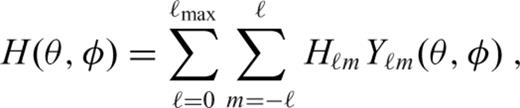
and symbols Δ′ and denote surface differential operators defined in spherical coordinates θ and φ as follows:

16

17

For the case considered here, when the shell is deformed due to a surface topography load h and buoyancy from deflection w of an internal density interface, q takes the form

18

For a homogeneous shell of constant thickness, D and α are constants and the solution of eqs (13) and (14) reduces to eqs (9)–(12), see Beuthe (2008). However, in a more general case when the elastic thickness and/or Young's modulus vary laterally, D and α are functions of θ and φ, and eqs (13) and (14) must be solved numerically (see appendix A for details). This numerical solution is hereinafter referred to as TSA-B.

2.3 Spectral solution for a thick shell of constant thickness

If the thickness of the shell does not vary with θ and φ, eqs (1)–(4) can be solved directly in 3-D geometry, that is, without using the thin shell approximation. The radial displacement w then depends not only on lateral coordinates but also on radius r. To solve the eqs (1)–(4), one only needs to slightly modify the spectral methods developed to study the viscoelastic deformation of the Earth (e.g. Sabadini & Vermeersen 2004) or the dynamic geoid (e.g. Hager & Clayton 1989). Here we use the semi-spectral method described by Golle et al. (2012) which has been generalized for compressible materials. The method (hereinafter called SSM) can be used to compute small deformations of a shell of arbitrary thickness with high accuracy and low computational costs. However, the method fails if the thickness of the shell varies laterally or if the material parameters E and ν depend not only on radius but also on θ and φ. The use of a finite element method is then more convenient.

2.4 Finite element solvers

The problem of deformation of an elastic shell of variable thickness was implemented in two numerical finite element software tools—Comsol Multiphysics (version 4.2a, www.comsol.com) and Elmer (http://www.csc.fi/elmer). In both cases, we used standard modules for linear elasticity in axisymmetric geometry, reducing effectively the problem to a 2-D one, which allows for reasonably high spatial resolution. We decided to use two different software tools and thus obtain two independent finite element solutions in order to at least empirically assess and control the error of the finite element approach; the solutions will be referred to as FEM-C and FEM-E for Comsol and Elmer, respectively.

The discrete problem was solved on non-structured triangular meshes, which were first generated in Comsol and then converted to Elmer (using the ElmerGrid tool) to assure the consistency and the comparability of both finite element solutions. As the basis functions we picked triangular second-order Lagrange elements (P2). The typical size of the problem was ∼10⁴ elements corresponding to approximately ∼10⁵ unknowns, allowing the use of direct solvers in both software packages. We performed mesh-refinement resolution testing of both FEM solvers and a fast numerical convergence was obtained even for very coarse initial meshes. This implies that the chosen resolution is fully sufficient.

3 Inherent Limitations of the Thin Shell Approximation

The thin shell approximation is primarily based on the assumption that the displacement is constant across the shell and that σ_rr is significantly smaller than σ_θθ and σ_φφ (for more details, see, e.g. Kraus 1967; Beuthe 2008). Although these assumptions are well satisfied if d≪R and the topographic loads are of wavelength λ≫d, one should always keep in mind that the thin shell solution is only approximate. For example, the estimates of the current elastic lithospheric thickness on Mars range between 100 and 300km (Grott & Breuer 2010), yielding d/R between 0.03 and 0.1 and d/λ between 0.05 and 0.15 (for λ corresponding to the load at harmonic degree 10). These values indicate that the error of the thin shell approximation may not be negligible. In this section and the section that follows, we attempt to quantify the accuracy of the thin shell approximation by comparing it with the solution obtained using a fully 3-D approach.

We consider a shell of constant thickness corresponding in outer radius to Mars (Table 1) deformed by a harmonic load induced by topography h_ℓ(θ) =AY_ℓ0(θ), with A = 1000 m. For a given topographic load h_ℓ and given parameters R, d, E, ν, ρ_c and ρ_m (see Table 1), the thin shell solution (TSA-T, Section 2.2) is fully characterized by a single value of the spherical harmonic coefficient w_ℓ. In contrast, the solution obtained for a shell of finite thickness (SSM, Section 2.3) is a function of radius, w_ℓ = w_ℓ(r), and depends also on the depth of the density interface t_c. The values of w_ℓ corresponding to topographic loads at degrees 2–50 computed for different thicknesses of the shell (d =10, 50, 100 and 250km) using the thin shell approximation are shown in Fig. 1. We compare them with the band of values corresponding to the SSM solutions obtained at different radii (r ranging from R−t_c to R) and for all admissible values of crustal thickness (t_c between 0 and d). The thickness of the band thus gives a rough estimate of the maximum error of the thin shell solution. Note, however, that the error may be even larger because parts of the TSA-T curve lie outside the band of the SSM solutions (Fig. 1 detail).

Table 1

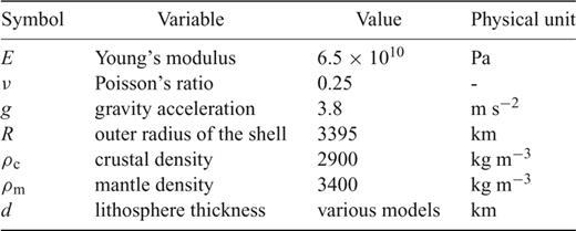
Model parameters.

Open in new tabDownload slide

Figure 1

Dependence of radial displacement coefficient w_ℓ on harmonic degree ℓ of the topographic load for different shell thicknesses, computed using the fully 3-dimensional SSM approach and thin shell approximation TSA-T.

Open in new tabDownload slide

To assess the role of parameter t_c, we compare the SSM solutions obtained for two end-member values of t_c, namely t_c = 0 (denoted by abbreviation BT—‘buoyancy top’) and t_c = d (BB—‘buoyancy bottom’). The radial dependence of the SSM solution is then illustrated by plotting the values of coefficient w_ℓ at the surface (r = R, denoted by DT—‘displacement top’) and at the base of the shell (r = R−d, DB—‘displacement bottom’). In the following, the abbreviation DT-BB refers to the SSM solution obtained at the surface for t_c = d, DT-BT is the solution obtained at the surface for t_c = 0, and DB-BB denotes the solution at the base of the shell obtained for t_c = d.

The effect of parameter t_c on the radial displacement at the surface is demonstrated in Fig. 2. The absolute value of the difference between the DT-BT and DT-BB solutions monotonically decreases with increasing degree. The rate of the decrease depends on the thickness of the shell, and it is larger for thick shells than for shells of small thickness. This trend can be attributed to the fact that, for a large thickness of the shell, the topography at high degrees is mostly supported by elastic stresses while the buoyancy effect of the density interface becomes negligible. In contrast, the buoyancy is a dominant mechanism maintaining the topographic loads even at high degrees if the thickness of the shell is sufficiently small. The extent of the radial variations in displacement within the shell is illustrated in Fig. 3, where we plot the coefficients w_ℓ obtained for t_c = d computed at the surface (DT-BB) and at the base of the shell (DB-BB). At low degrees, the differences between the two cases are one order of magnitude smaller than in Fig. 2. At high degrees, however, the differences due to variable radius are comparable to or even larger than those due to different values of crustal thickness t_c. For further discussion of the accuracy of the thin shell approximation, the reader is referred to, for example, Zhong & Zuber (2000) and Beuthe (2008).

Figure 2

(a) Radial displacement coefficient w_ℓ at the surface (DT) as a function of harmonic degree ℓ of topographic load computed by SSM for four different shell thicknesses d and two end-member crustal thicknesses, t_c = 0 (BT) and t_c = d (BB). (b) Difference between the DT-BB and DT-BT solutions.

Open in new tabDownload slide

Figure 3

(a) Radial displacement coefficient w_ℓ as a function of harmonic degree ℓ of topographic load computed by SSM at the base of the shell, r = R−t_c (DB), and at the surface, r = R (DT). The results are plotted for four different shell thicknesses d and crustal thickness t_c = d (BB). (b) Difference between the DB-BB and DT-BB solutions.

Open in new tabDownload slide

4 Comparison of Different Methods

We now compare different methods designed to compute the deformation of a shell with variable thickness, namely the method proposed by Beuthe (TSA-B, Section 2.2) and the finite element methods (FEM-C, FEM-E) described in Section 2.4. To assess their numerical properties, we first apply them to the elastic shell of constant thickness for which a highly accurate spectral solution (SSM) is available.

4.1 Elastic shell of constant thickness

If the thickness of the elastic shell does not vary laterally, the topographic load at degree ℓ induces deformation which is fully described by radial displacement w_ℓ at the same degree. This allows the accuracy of the computational methods to be tested in the spectral domain, that is, in the same way as in Section 3. The only inconvenience of this approach is that, in the case of the finite element methods, the harmonic loading function must be first evaluated on a grid, and, after performing the computation, the resultant radial displacement must be expressed in terms of a spherical harmonic function. The transformation from spectral to spatial domain and back produces an additional numerical error, but as we will see, this error is negligible if the grid step is significantly smaller than the wavelength of the spherical harmonic function.

Fig. 4 illustrates the accuracy of different methods (TSA-T, TSA-B, FEM-E and FEM-C) with respect to SSM which is assumed here to have a negligible error (note that the spectral representation in lateral direction is effectively equivalent to a finite-difference scheme of the same order as the spectral cut-off degree, cf.Fornberg 1998). The geometry and material properties of the shells used in testing the accuracy are the same as in Section 3. The quantity Δw_ℓ, plotted on the vertical axis, is defined as a difference between the radial displacement at degree ℓ obtained by the tested method and the radial displacement computed at the same degree using SSM for t_c = 0 at r = R (DT-BT). The shaded area indicates the dispersion of the SSM solution due to its dependence on r and t_c (cf.Section 3). It is confined by two curves, Δw_ℓ = 0 and the curve corresponding to the difference between the SSM solutions obtained for DB-BB (r = R−d, t_c = d) and DT-BT (r = R, t_c = 0).

Figure 4

Error of radial displacement coefficient w_ℓ with respect to the SSM DT-BT solution plotted as a function of harmonic degree ℓ of topographic load. Four different elastic shell thicknesses d are considered: 10km (a), 50km (b), 100km (c) and 250km (d).

Open in new tabDownload slide

The methods based on the thin shell approximation (TSA-T, TSA-B) are represented by single curves. The curves are identical, thus confirming that the TSA-B method, developed to study a shell of variable thickness, reduces to TSA-T if the thickness of the shell is constant (cf.Beuthe 2008). The behaviour of the errors for both methods depends on two factors—the thickness of the shell and the harmonic degree of the load. For harmonic degrees below a certain threshold, the error is confined to the dispersion-error region (shaded) and thus can be explained solely by dependence of the exact (SSM) solution on r and t_c. Above this threshold, the error leaves the shaded region, manifesting that the physical assumptions of the thin shell approximation become violated. The position of the threshold depends monotonically on the shell thickness and is decreasing with increasing shell thickness. Note that for low degrees, the TSA solutions are rather close to the SSM solution obtained for t_c = 0 (BT) while their error is the largest for t_c = d (BB). This indicates that the accuracy in determining the geoid at low degrees using the thin shell approximation decreases with increasing depth of the density interface since the error in the geoid height is directly proportional to the error of w_ℓ if ℓ is small (cf. eq. 8)

19

At high degrees the error of the geoid decreases due to the diminishing of the geometrical factor [(R−t_c)/R]^ℓ+2.

The accuracy of each of the finite element methods (FEM-C, FEM-E) is illustrated in Fig. 4 by the two pairs of curves corresponding to the DT-BT and DB-BB cases. These curves frame the borders of the shaded area, thus confirming the high accuracy of both methods. For small values of d (≤10km), the accuracy of the finite element methods is similar to that of the thin shell methods, but it grows significantly higher for larger values of d. Both finite element methods are comparable in accuracy, but a detailed inspection of the results reveals that FEM-C is slightly more accurate than FEM-E where we are not able to reduce certain minor spurious oscillations in displacement in the case of very thin shells (Fig. 4a). That is why FEM-C will be used as a reference method in the next section, where we deal with a shell of variable thickness for which the semi-spectral method can no longer be used.

4.2 Elastic shell of variable thickness

The numerical properties and accuracy of the computational methods are tested on three synthetic models of elastic shells with variable thickness (Fig. 5). The outer radius and material parameters of the shells are the same as in the previous sections (see Table 1). The shells are axisymmetric with thickness d ranging from 50 to 200km in model I and from 50 to 150km in models II and III. Model I consists of two hemispheres of contrasting thicknesses separated by a sharp (but smooth) transition while models II and III exhibit harmonic variations of elastic thickness with a wavelength of 180° and 36°, respectively. Each shell is deformed by the same topographic load as in Section 3 (i.e. harmonic topography with amplitude 1000 m). As the thickness of the shell varies laterally, its response to harmonic loading is more complex than in the case of a shell with uniform thickness: a load of a given degree now induces deformation not only at the same degree but, in general, at all other degrees. That is why we present the resultant radial displacement in the spatial domain, that is, as a function of θ, and not in terms of the spectral coefficients as in previous sections.

Figure 5

Elastic thickness models used in Section 4.2.

Open in new tabDownload slide

The reference (‘accurate’) method is now FEM-C, while the tested methods are FEM-E, TSA-B and TSA-T. Since we are performing the comparison in the spatial domain, a cut-off degree has to be chosen for both spectral methods. Investigating the power spectra of parameters D and α, defined in Section 2.2, for models I–III, a cut-off degree ℓ_max = 100 was found to provide sufficient accuracy. In contrast to FEM-C, FEM-E and TSA-B, designed to address the deformation of a shell with variable thickness, TSA-T was originally developed to study the case of a uniform thin shell. Its application is, however, extremely simple in comparison with the other methods, and it is thus tempting to use it also for thin shells of variable properties. To estimate the flexure of a shell with variable thickness, we use TSA-T in the simplest possible way: the radial displacement at a point of colatitude θ and longitude φ is computed using eqs (9)–(12) as if the shell was of uniform thickness given by d(θ, φ), that is, we take

20

The results obtained for the three model shells described above and for the different loading functions are shown in Figs 6–8. In each figure, rows 1–4 correspond to the loading imposed at degrees 2, 5, 8 and 15, respectively. The panels on the left show the radial displacement w = w(θ) obtained using different computational methods, while the right panels illustrate errors of the individual solutions with respect to the DT-BT solution computed by the reference method (FEM-C). The area in yellow shows the dispersion of the reference FEM-C solution due to its dependence on r and t_c. It is bounded by Δw = 0, corresponding to the zero error of the DT-BT solution from one side, and by Δw = w^DB-BB−w^DT-BT, corresponding to the difference between the DB-BB and DT-BT solutions from the other.

Figure 6

Displacement w (left-hand side) and its absolute error Δw with respect to FEM-C (DT-BT) (right-hand side) as a function of θ for elastic thickness model I. The harmonic loading is imposed at degrees 2 (panels a, e), 5 (b, f), 8 (c, g) and 15 (d, h). The displacement w and error Δw are plotted by colour lines corresponding to different computational methods. The yellow envelope illustrates the dispersion of reference FEM-C method. Elastic thickness model used to calculate w is indicated by the thin black line with a scale plotted on the right.

Open in new tabDownload slide

Figure 7

The same as in Fig. 6 but for model II.

Open in new tabDownload slide

Figure 8

The same as in Fig. 6 but for model III.

Open in new tabDownload slide

Inspection of the left panels in Figs 6–8 suggests that all of the solutions, including the TSA-T used in local approximation (eq. 20), are rather close to each other, and the differences among them are strikingly small. As could be expected from the tests performed in Section 4.1, there is basically no difference between the FEM-E and FEM-C solutions. This is obvious from the fact that, in the right panels of Figs 6–8, the two red curves corresponding to the FEM-E solutions obtained for the DT-BT (full line) and DB-BB (dashed line) configurations perfectly frame the yellow area corresponding to the FEM-C solutions.

The errors of the TSA-B method (green lines) with respect to FEM-C are of a similar order as the errors obtained for the thin shell approximation in the case of a shell of uniform thickness (cf. Fig. 4). Related to the maximum amplitude of the radial displacement, the error does not exceed a few percent. The relative accuracy is high especially in regions where the thickness of the shell is small, and it deteriorates as the thickness of the shell increases (cf. for example left and right parts of panels in Fig. 6).

The accuracy of the TSA-T method in local approximation (blue lines in Figs 6–8) is rather sensitive to the wavelength of the loading function and the rate of change of shell thickness d with θ. The errors are largest if the wavelength of the load is comparable with or larger than the characteristic length of function d(θ), which is well demonstrated in the top right panels of Figs 6–8 corresponding to degree-2 load. For higher degree loads, the TSA-T solution is almost identical with TSA-B, except for the sharp transitions between the regions of constant thickness in model I (see bottom panel in Fig. 6), or the regions where the local value of d differs significantly from the average value of d in the near field—in polar regions (models II and III) and at local thickness extrema (model III)—see Figs 7 and 8. In general, the estimates of the radial displacement obtained using TSA-T are strikingly accurate. This suggests that the TSA-T method, which is very simple and computationally cheap, can provide a reasonably good, first-order estimate of the radial displacement even for shells with variable thickness, although it was originally designed for uniform thin shells.

5 Effect of Shell Thickness Variations on the Local Deformation

The results computed using the TSA-T method for a shell of variable thickness and their close proximity to those obtained by TSA-B indicate that local deformation of the shell is rather insensitive to shell thickness variations in the far zone. To better understand this issue, we evaluate the average relative errors of these two methods in different regions of model I. The error δw corresponding to a load at degree ℓ is defined as follows:

21

where θ₁ and θ₂ are the endpoints of the region under consideration, Δw(ℓ, θ) is the absolute error of the displacement computed for load of degree ℓ in the point with colatitude θ and

22

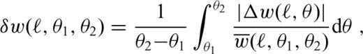
As in the previous section, the absolute error Δw is evaluated with respect to the FEM-C (DT-BT) solution. We note that the expression in the integrand of eq. (21) differs from the usual definition of the relative error (Δw/w) which would diverge in points with zero displacement.

Fig. 9 shows the average relative error δw computed for different regions of model I in dependence on degree ℓ of the loading function. Panels a, b and c show δw obtained from eq. (21) by integrating over the interval (0°, 80°), (100°, 180°) and (80°, 100°), respectively. In the regions where d does not change laterally (Fig. 9, panels a and b, corresponding to d =200km and 50km, respectively), the relative error of TSA-T (blue line) is almost identical to that of TSA-B (green line), except for very low degrees with wavelength larger than or comparable to the size of the domain (∼80°). The relative error of both methods is significantly larger for d =200km than for d =50km (note different scales in panels a and b of Fig. 9). This is comprehensible since the amplitude of the radial displacement w generally decreases with increasing shell thickness, whereas the error Δw of the thin shell approximation increases with increasing d/R. Starting from certain degree (ℓ∼ 10 in Fig. 9a and ∼30 in Fig. 9b) the relative error increases which is associated with the expected deterioration in the accuracy of the thin shell approximation for larger values of d/λ (cf.Section 3).

Figure 9

The average relative error δw, eq. (21), as a function of harmonic degree ℓ for different parts of model I. (a) Left part of the model (θ going from 0° to 80°) with elastic thickness d = 200km; (b) right part of the model (100°–180°) with d = 50km; (c) transition region (80°–100°) with d gradually decreasing from 200km to 50km.

Open in new tabDownload slide

Fig. 9(c) shows the relative errors of the methods for the transition region, θ∈ (80°, 100°), in which the shell thickness gradually changes from 200 to 50km. While the errors of TSA-T and TSA-B are basically the same if d is constant (Figs 9a and b), in the region of pronounced thickness variations (Fig. 9c), the TSA-B solution is found to be significantly more accurate than the TSA-T solution, especially for intermediate degrees.

The above results can be generalized as follows: the local deformation of the shell is insensitive to the shell thickness variations if the wavelength of the load is significantly smaller than the characteristic length scale of the thickness variations. This implies that the radial displacement induced by a global load at the point with shell thickness d can be estimated by computing the radial displacement at this point for the shell of uniform thickness d induced by the same load. This approach may provide a reasonable first-order estimate of radial displacement even for very large wavelengths of the load (note that in Fig. 9δw computed for ℓ= 2 never exceeds 10 per cent). However, the accuracy of the above approximation deteriorates in regions where the rate of change of d is large (Fig. 9c) or where the local value of d at the given point does not represent the mean thickness of the shell in its vicinity (e.g. if the point coincides with a local extremum of the shell thickness).

6 Elastic Lithosphere of Variable Thickness in Models of Mantle Flow

So far, we have dealt with an elastic shell deformed due to a topographic load imposed at its surface. Another potentially important source of shell deformation are forces induced by viscous flow in the mantle beneath the elastic lithosphere (Zhong 2002; Roberts & Zhong 2004; Golle et al. 2012).

If we neglect the elastic behaviour of the uppermost part of the body and assume that both the crust and the mantle are viscous, we can estimate the surface topography h^vis induced by mantle flow from the radial component of the traction vector at radius r = R:

23

where σ_rr is obtained from the solution of the Stokes problem with non-penetration (v_r = 0) and free-slip (σ_rθ =σ_rφ = 0) boundary conditions at the upper surface (e.g. Hager & Clayton 1989).

Zhong (2002) has suggested that, for a radially stratified body, the dynamic topography h^el for an elastic shell resting above a viscous layer can be obtained by superposition of the viscous and elastic responses in the spectral domain. If the elastic shell is sufficiently thin for the thin shell approximation (Turcotte et al. 1981) to be valid, this approach allows one to simply compute the elastic dynamic topography h^el from the purely viscous case h^vis by the following correction in the spectral domain:

24

with defined as

25

where

26

27

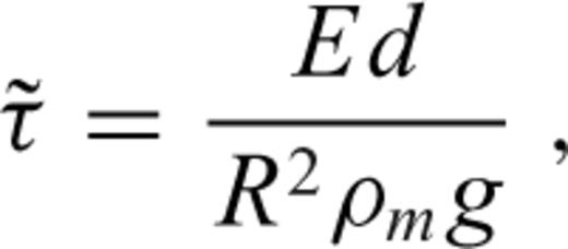
The coefficient characterizes the flexural response of the elastic shell to a surface radial force T_ℓ of degree ℓ normalized with respect to the corresponding isostatic deflection,

28

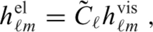
where is the spherical harmonic coefficient of the radial displacement induced at the surface of the elastic shell by the same radial force T_ℓ (cf. eqs (10)–(12) in Section 2.2). Derivation of eqs eqs (24)–(28) can be found in appendix B.

It should be emphasized, however, that the above formalism is strictly valid only for a thin homogeneous elastic shell with a uniform thickness which is the same as the thickness of the stagnant lid in the viscous model. If this is satisfied, one can indeed prove that a general (not necessarily radial) surface force acting on the bottom boundary of the elastic and viscous shell induces radial deflections h^el and h^vis, respectively, which are related by eq. (24).

We will now test whether the approach of Zhong (2002) can be generalized to capture also the case with laterally variable lithospheric thickness. Using the finite element solver FEM-C we will investigate the relationship between viscous and elastic deformation for a shell of variable thickness. In particular, we will test whether the dynamic topography obtained for a viscous shell of a given geometry can be corrected for the effect of elasticity in a way analogous to eq. (24), that is, by applying a spectral solver (TSA-B or TSA-T) to an elastic shell of the same geometry. We consider a model of shell thickness variations (thin black lines in Fig. 10) which combines the properties of models I and III used in Section 4.2 by including both long- and intermediate-wavelength features.

Figure 10

Dynamic topography h^el of the elastic shell induced by forces acting at its base (left-hand side) and its absolute error with respect to FEM-C (right-hand side) as a function of θ. The colour lines show the results obtained by different methods. The model of elastic thickness variations is illustrated by the thin black line. Individual rows correspond to loading functions imposed at degree 2 (panels a, e), 5 (b, f), 8 (c, g), and 15 (d, h).

Open in new tabDownload slide

Our testing strategy is as follows. In the first step, we assume that the shell is elastic (E = 6.5 × 10¹⁰ Pa, ν= 0.5) with uniform density ρ_m = 3400 kg m^-3, and, using FEM-C, we solve the following (incompressible) elastic deformation problem:

29

30

31

The boundary conditions are topography load at the upper surface

32

and traction force at the bottom surface

33

The resulting radial displacement at the surface (‘elastic surface topography’h^el) obtained for

34

imposed at degrees ℓ= 2, 5, 8, 15 with Pa, is plotted in red in the left panels of Fig. 10. The geometric scaling factor in expression for K is to ensure zero loading at degree one, which otherwise would require special treatment. This solution will be considered as the reference one.

In the second step, we use FEM-C to compute the viscous dynamic topography h^vis, eq. (23), for a homogeneous viscous shell of the same geometry. We solve the following equations

35

36

37

where v is the velocity, p is the pressure and η is the viscosity. We consider impermeable free-slip upper boundary

38

39

and the prescribed traction force (same as in the first step) at the bottom boundary

40

We note that the dynamic topography obtained for the viscous shell h^vis (not shown in Fig. 10) differs from the elastic topography h^el found in the previous step.

In the third step, we use the dynamic topography h^vis computed in the second step, and we correct it for the elastic effect. As a result, we should obtain the same shape of the surface as in the elastic case. The correction is performed using the thin shell approximation TSA-B developed by Beuthe (2008), that is, by solving eqs (13) and (14) discussed in Section 2.2, with the force q in eq. (13) of the form

41

corresponding to the forces T and Q from appendix B. The surface topography obtained in this way (green lines in Fig. 10) indeed agrees rather well with the FEM-C solution obtained directly for the elastic shell in step one. The error with respect to FEM-C (right panels of Fig. 10) does not exceed a few percent of the maximum amplitude and is comparable in size with the error of the thin shell approximation discussed in Section 4.

A first order estimate of the topography induced by forces acting at the base of the elastic shell with variable thickness can be computed using the TSA-T method with the coefficient , eq. (25), depending on the local thickness of the shell (cf. eqs 20 and 24)

42

In Fig. 10, the surface topography obtained for our axisymmetric model using eq. (42) is plotted as blue lines. The accuracy of the TSA-T estimate is rather good and comparable to the TSA-B solution in the northern hemisphere where the shell thickness does not change. But even in the southern hemisphere, where we impose large shell thickness variations, TSA-T provides an acceptable estimate of the surface topography, with accuracy up to 10 per cent with respect to the maximum amplitude.

The above results suggest that the method for the elastic correction of a viscous dynamic topography proposed by Zhong (2002) can also be applied to models with a stagnant lid of variable thickness (cf.Zhong et al. 2003). The first-order estimate of the dynamic topography corrected for the elastic lithosphere effect can be obtained using the traditional spectral method developed by Turcotte et al. (1981) and employed also in the work of Zhong (2002). The method must be slightly modified (eq. 42), but its application remains straightforward. A more accurate surface topography can be obtained by solving the equations presented by Beuthe (2008). Owing to the thin shell approximation, the number of unknowns in the equations is not large and the spectral solution is thus less expensive than application of a finite element method to a shell of finite thickness.

7 Concluding Remarks

In this paper, we have analysed the deformation of an elastic spherical shell with variable thickness. We compared two approximate thin shell methods (Turcotte et al. 1981; Beuthe 2008) with methods based on either semi-spectral or finite element discretization of the original problem of finite thickness. For a Mars-like body subject to harmonic loading, we inspected the accuracy of the methods especially at low to intermediate degrees corresponding to the prevailing low-degree character of the observed topography of terrestrial planets (typical linear log–log spectral decay, see, e.g. Turcotte 1987; Čížková 1996; Pauer et al. 2006).

Starting with the case of a shell of uniform thickness, we estimated the inherent inaccuracy of the thin shell methods, arising from both the geometrical and physical assumptions within the thin shell approach. Both thin shell methods coincide in this case, and their errors for low degrees (ℓ≤ 20) do not exceed 5 per cent for small shell thicknesses (d≤50km) and 10 per cent for thick shells (d∼ 250km; see also Figs 1–4).

For a shell of variable thickness, the method of Beuthe (2008) performs with accuracy comparable to the uniform thickness case. When the wavelength of thickness variations is large compared to the wavelength of the load, the errors arise mainly from the thin shell approach—they are confined to regions with high local shell thickness and do not exceed 5–10 per cent (Figs 6 and 7). For models with highly variable thickness, the errors increase but, in general, do not exceed 15 per cent (Figs 6 and 8). It is important to note that this method is essentially 2-D and the solution thus computationally much less demanding than that of the original 3-D problem. Moreover, in the case of a solely normal load, the problem reduces from five to only two coupled partial differential equations, which can be easily solved by the spectral approach outlined in appendix A.

Motivated by the simplicity and good performance of the approach of Turcotte et al. (1981) for shell of uniform thickness, we introduced and investigated also its straightforward extension to the case of variable shell thickness. This approach performs generally more poorly than the approach of Beuthe (2008), especially in regions where the shell thickness varies significantly, but, quite surprisingly, it provides a rather good and computationally very cheap first-order estimate of the resulting displacement (Fig. 9).

Finally, concerning also the force coupling with mantle convection below the shell, we proposed an extension of the concept of Zhong (2002) to the case of a shell of variable thickness. We investigated two methods of spectral correction of a viscous solution to the problem, based on either Beuthe (2008) or Turcotte et al. (1981). The results are again satisfactory with the errors comparable with the case of normal surface loading (Fig. 10).

To sum up, the thin shell methods have proven to be quite reliable and, due to computational effectiveness, very useful tools to estimate the elastic deformation of a spherical shell with variable thickness for general surface and bottom loading. The method of Beuthe (2008) remains very accurate even in regions with high local thickness variability, where the method based on the technique of Turcotte et al. (1981), despite being less accurate, still provides a reasonable estimate and benefits from its tremendous computational simplicity.

Acknowledgments

The authors thank Mikael Beuthe and an anonymous reviewer for their comments and suggestions and Craig Bina for reading the manuscript. The work was supported by Charles University grants GAUK-259099 and SVV-2012-265308, grant No. MSM0021620860 and by the Jindřich Nečas Center for Mathematical Modelling, project LC06052, both financed by the Ministry of Education, Youth and Sports of the Czech Republic.

Appendices

Appendix A: Spectral Solution for A Thin Shell of Variable Thickness

To solve eqs (13) and (14) derived by Beuthe (2008), we first discretize the unknown functions w(θ, φ) and F(θ, φ) in terms of spherical harmonic series

(A1)

(A2)

where w_ℓm and F_ℓm are the spherical harmonic coefficients to be determined, Y_ℓm are the fully normalized complex spherical harmonic functions (e.g. Edmonds 1974; Jones 1985; Varshalovich et al. 1988) and

(A3)

with ℓ_max being the cut-off degree. The choice of ℓ_max depends on the properties of the function d (shell thickness), used in evaluating the parameters D and α (see below). All results presented in the main text have been obtained for ℓ_max = 100 guaranteeing high accuracy of the solution for all considered models.

Before solving the equations, we express D and α in terms of spherical harmonic expansions,

(A4)

(A5)

where D_ℓm and α_ℓm are the spherical harmonic coefficients which can be determined by numerical integration of d over the unit sphere,

(A6)

(A7)

with the asterisk denoting complex conjugation.

To transform the partial differential eqs (13) and (14) into a set of linear algebraic equations for unknown coefficients w_ℓm and F_ℓm, we must first apply the differential operators Δ′ and , eqs (16) and (17), to spherical harmonic functions in expansions (A1), (A2), (A4) and (A5) and then evaluate the products of appropriate spherical harmonic series. Following Beuthe (2008, 2010), we can write

(A8)

(A9)

where

(A10)

(A11)

The product of two spherical harmonic functions can be expressed as follows (Varshalovich et al. 1988)

(A12)

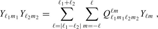
where the Gaunt coefficients can be rewritten using the Clebsch-Gordan coefficients,

(A13)

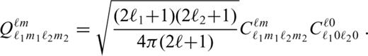
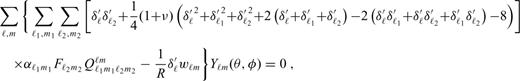
The Clebsch-Gordan coefficients are non-zero only if ℓ, ℓ₁ and ℓ₂ are non-negative, m = m₁+m₂, |m|≤ℓ, |m₁|≤ℓ₁, |m₂|≤ℓ₂, and |ℓ₁−ℓ₂|≤ℓ≤ℓ₁+ℓ₂. Substituting eqs (A1), (A2), (A4) and (A5) in eqs (13) and (14) and applying eqs (A8)–(A12), we obtain

(A14)

(A15)

where h_ℓm are the known coefficients in the spherical harmonic expansion of topography. Since eqs (A14) and (A15) are valid for any θ and φ, the expressions in the curly brackets must be identically equal to zero. Eqs (A14) and (A15) can thus be rewritten in terms of two coupled sets of linear algebraic equations for unknown coefficients w_ℓm and F_ℓm,

(A16)

(A17)

where

(A18)

(A19)

(A20)

(A21)

(A22)

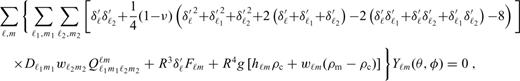
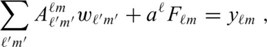
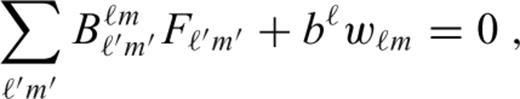
Note that in order to minimize the numerical errors caused by operations with large numbers, eq. (A14) was divided by , where d₀ is some reference (constant) thickness, and eq. (A15) was multiplied by R. In the axisymmetric geometry, indices m, m₁ and m₂ are equal to zero, and the total number of unknowns reduces to 2(ℓ_max+1). All sums over indices M and m′ in eqs (A16)–(A18) and (A21) vanish, and the Gaunt coefficients in eqs (A18) and (A21) can easily be evaluated using the analytical formula for the Clebsch-Gordan coefficients with zero m indices (Varshalovich et al. 1988):

(A23)

if 2K≡ℓ+ℓ′+L is an even number, and for odd values of 2K.

Appendix B: Derivation of The Flexural Response Coefficient

We start from eq. (3) in Willeman & Turcotte (1982) for the thin shell radial deformation w under normal force p

(B1)

Decomposing p into bottom and surface components T and Q, respectively, expanding w, T and Q into spherical harmonic series, and taking into account linearity of the problem, we arrive at the following spectral relationship

(B2)

where

(B3)

(B4)

(B5)

In Section 6, we investigate the case when the bottom force T_ℓm is prescribed. This force induces surface deflection w_ℓm which is associated with surface reaction force Q_ℓm,

(B6)

We wish to compare the dynamic topographies in the purely elastic and purely viscous cases. In the viscous case, the dynamic topography h^vis is only supported by the bottom force T,

(B7)

Realizing that the elastic dynamic topography h^el is now just the deflection w, and substituting eqs (B6) and (B7) into eq. (B2), we obtain the sought relation (24) with given by eq. (25).

References