Crustal structure of the British Isles and its epeirogenic consequences

Summary

1 Introduction

The British Isles sit on the northwestern margin of the European continent and have a diverse solid geology, which is the result of a punctuated history of subsidence and tectonic activity (Woodcock & Strachan 2000). Orogenic and rifting processes have given rise to a collage of geological terranes but the oldest outcrop generally occurs in the northwest: Mesozoic and Cenozoic strata young to the east and southeast. Here, we are especially interested in the Cenozoic to present-day evolution of a region, which includes the British Isles. By the end of Cretaceous times, it is generally thought that a marine incursion had flooded this region and that topographic relief was modest. During Early Cenozoic times, this palaeogeography changed rapidly when extrusive and intrusive basaltic magmatism affected a north–south belt. Brodie & White (1994) suggested that regional magmatism was accompanied by a component of underplating which triggered epeirogenic uplift. Later, White & Lovell (1997) argued that the history of Palaeogene magmatism caused phases of uplift and denudation which gave rise to a series of clastic submarine fan deposits which occur in the North Sea and Faroe-Shetland basins. Mass balance calculations suggest that ∼0.5 × 10⁶ km³ of material was eroded from the British Isles. A similar volume of clastic sedimentary rock has been mapped offshore (Jones et al. 2002). During Neogene times, several minor phases of epeirogenic uplift probably occurred, although these phases are difficult to date with accuracy. Jones et al. (2002), Bott & Bott (2004) and Arrowsmith et al. (2005) have all suggested that a warm buoyant finger of asthenospheric mantle protrudes south from the Icelandic plume beneath the lithospheric plate, providing dynamic topographic support and generating the well-known belt of small earthquakes. If correct, this suggestion implies that the Icelandic plume continues to have an important influence on vertical movements of the British Isles since its inception at 62 Myr.

In contrast, Hillis et al. (2008), Holford et al. (2009) and Stoker et al. (2010) argue that the chronology and distribution of Cenozoic denudation can be accounted for by multiple phases of plate shortening. They suggest that four episodes of uplift and erosion occurred during Cenozoic times and that these episodes were caused by compressional uplift triggered by fluctuating intraplate stress fields. In their view, neither magmatic underplating nor dynamic topography driven by convective upwelling are significant drivers of regional uplift.

The crustal and lithospheric structure of the British Isles are a key constraint which should enable us to discriminate between these rival epeirogenic and orogenic models. If magmatic underplating did occur in Palaeogene times, we would expect to find fast velocities in the lower crust beneath the surficial trace of basaltic magmatism. If present-day dynamic support is important, it should also be possible to estimate its amplitude by analysing the relationship between average topographic elevation and crustal density structure. Here, receiver function analyses of earthquake records from 51 three-component broad-band seismometers are used to determine the onshore crustal structure of the British Isles. The resultant velocity-depth profiles have been combined with crustal models based on controlled-source experiments to build a detailed picture of onshore and offshore crustal structure.

2 Receiver Function Analysis

Earthquake records of three-component, broad-band seismometers can be used to determine the 1-D structure of the crust and mantle by calculating receiver functions (Langston 1979). This method exploits mode conversions of earthquake energy within the lithosphere to deconvolve effects of the earthquake source and path through the Earth from the incident wave train. The deconvolution technique isolates the shear wave velocity structure beneath the receiver. When an incoming P wave encounters a velocity contrast (e.g. the Moho) some proportion of the incident energy is converted into an S wave at this interface. Since S waves travel more slowly, this mode conversion and any subsequent reverberations arrive at the receiver after the direct P-wave arrival. The P-wave arrival is prominent on the vertical component and the later P-to-S converted arrivals and reverberations are manifest on the radial component. These arrivals are not visible on a seismogram since they occur within the P-wave coda and have small amplitudes. However, they can be isolated and identified by calculating the receiver function for a given event. Signal-to-noise ratio is improved by stacking many such events at each station. Stacked receiver functions are used to calculate the velocity structure of the crust and mantle by a combination of forward and inverse modelling.

In the British Isles, a small number of previous receiver function studies have been carried out. Shaw Champion et al. (2006) used earthquake records from five three-component broad-band seismometers located along an existing seismic wide-angle experiment to calculate the velocity structure of the crust in northern England and to compare it with the wide-angle model. Landes et al. (2006) used a temporary array of shorter period three-component seismometers to determine the crustal structure of southwest Ireland. Tomlinson et al. (2006) carried out a more comprehensive study, in which they determined crustal structure at 28 locations from 1493 receiver functions. Unfortunately, only nine of their 34 three-component seismometers are broad-band instruments suitable for receiver function analysis. Short period instruments yield receiver functions which are plagued by high frequency oscillations due to the narrower band of frequencies used during deconvolution. Finally, Di Leo et al. (2009) analysed the temporary RUSH array of seismometers in northern Scotland.

Here, we build upon these earlier studies by analysing earthquake data from 51 three-component broad-band seismometers. Of these instruments, 42 are currently deployed and nine are from previous temporary deployments (Fig. 1 and Table 1). Data coverage is variable (e.g. 21 yr at ESK, 6 months at GNP) but the majority of stations have records for 3 yr, which is sufficient for our purposes. The five stations studied by Shaw Champion et al. (2006) have been included because additional data have become available. Some of the short period stations used by Tomlinson et al. (2006) have recently been upgraded to broad-band status and are included. We also use six stations from the temporary RUSH array, which operated for sufficiently long periods (Asencio et al. 2003; Bastow et al. 2007; Di Leo et al. 2009).

Figure 1

Simplified geological map of British Isles showing distribution of broadband, three component, seismometers used in this study. Labelled solid triangles – stations deployed during British Isles Seismic Experiment (BISE); open triangles – stations operated by BGS and by AWE-Blacknest; inverted solid triangles – stations operated by IRIS and by ORFEUS; inverted open triangles – temporary stations operated by IRIS. See Table 1 for additional information. Dark grey shading – Precambrian and Palaeozoic rocks; light grey shading – Mesozoic and Cenozoic sedimentary rocks; black shading – Cenozoic igneous rocks. Redrawn from Woodcock & Strachan (2000).

Open in new tabDownload slide

Table 1

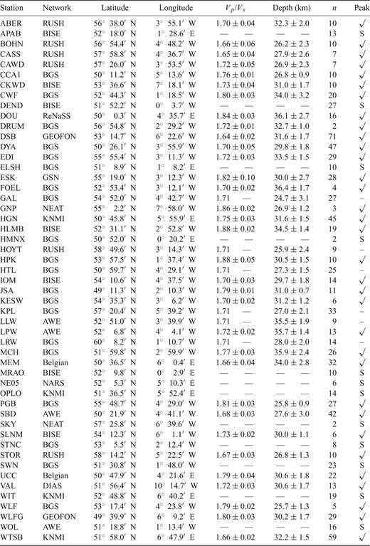
Summary of information for stations used in this study. Moho depths and average crustal V_p/V_s ratios were calculated from H - κ stacking. V_p/V_s ratio of 1.71 was assumed for stations without a clear P_s peak.

Open in new tabDownload slide

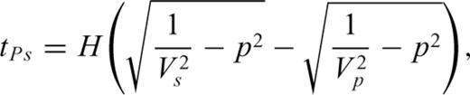
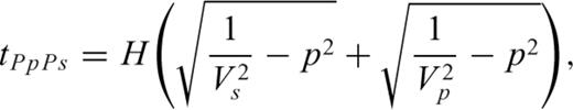
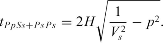
Seismograms were selected for each station by choosing events with body wave magnitudes >6, which occurred at epicentral distances of between 30° and 95° and have emergent P-wave arrivals (Fig. 2). The majority of events fulfilling these criteria occurred in Central America with westerly backazimuths and near Japan with northerly backazimuths. For each seismogram, a 100 s window of data was extracted, starting 25 s before the P-wave arrival (Kennett & Engdahl 1991). Horizontal seismograms were then rotated into radial and transverse components. These components were deconvolved in the time domain using the iterative method of Ligorría & Ammon (1999). Their approach improves the approximation to the receiver function for each iteration by adding a peak, convolving this approximation with the vertical component, and then comparing the result with the radial component. Typically, 200 iterations were carried out. We used a Gaussian width of two, which corresponds to a 90 percent cut-off at 1 Hz. This value gives an appropriate balance between noise and detail within a receiver function. Calculated receiver functions were inspected by eye and stable ones were identified for detailed analysis. In all, >3300 receiver functions were deemed suitable. A small selection of radial receiver functions are shown in Figs 3 and 4. In each case, Moho Ps arrivals at 3–4 s, PpPs multiples between 11–14 s, and the negative PpSs+PsPs multiples at 14–18 s are clearly visible.

Figure 2

Azimuthal equidistant projection centred on 55°N, 4°W and showing 1055 events located at angular distances of 30°–95° from stations plotted in Fig. 1. Distribution of backazimuths is not uniform: majority of events are from north and west quadrants.

Open in new tabDownload slide

Figure 3

Large selection of receiver functions calculated for two permanent stations (a) DSB and (b) ESK showing Moho conversions and multiples (Table 1). In each case, receiver functions are plotted as a function of backazimuth (BAZ), which is quoted in degrees. Peaks at 0 seconds – direct P arrivals. At DSB, a diffuse Ps arrival at 2–3 s and two coherent PpPs arrivals at 10.5 and 12.5 s are visible. At ESK, there is a clear Ps arrival at 4 s but mode-converted multiple energy is less emergent.

Open in new tabDownload slide

Figure 4

Small set of receiver functions calculated for stations (a) ABER, (b) CCA1, (c) CKWD and (d) HTL for carefully selected back-azimuthal ranges (BAZ, see Table 1). Ps and PpPs arrivals are visible at 2–4 s and 10–14 s, respectively. HTL has double PpPs and PpSs+PsPs arrivals (i.e. troughs at 14–18 s), indicative of two interfaces towards base of crust.

Open in new tabDownload slide

In southern Britain, some stations (e.g. APAB, DEND, ELSH, Fig. A1) have a delayed zero time peak, which is typically associated with a slow surface layer (e.g. sedimentary cover, ice cover; Zelt & Ellis 1999; Kumar et al. 2007). These stations are often sited on Cenozoic and Mesozoic sedimentary rocks, which are less consolidated than the Palaeozoic and Precambrian rocks elsewhere in the British Isles (Fig. 1). Some stations in Belgium and the Netherlands (e.g. NE05, OPLO and WIT, Fig. A1) also have delayed zero time peaks and regularly spaced arrivals on the receiver functions which are most likely sedimentary reverberations. These stations are difficult to model properly and have been omitted from our final crustal synthesis.

2.1 H−κ stacks

The H−κ stacking method of Zhu & Kanamori (2000), where H refers to crustal thickness and κ is the V_p/V_s ratio, was used to obtain initial estimates of crustal structure and composition (Fig. 5). This grid-search technique is easy to apply and it is a useful form of quality control before detailed modelling is carried out. Amplitude peaks on a receiver function represent the direct conversion arrivals, Ps, and multiple events, PpPs and PpSs+PsPs, which arrive after the direct conversion since they reflect at both the surface and Moho. Zhu & Kanamori (2000) showed that for crust which consists of a single layer of uniform velocity, Ps, PpPs and PpSs+PsPs arrival times are a function of the ray parameter p, the crustal thickness H, and the V_p/V_s ratio:

1

2

3

A subset of stable receiver functions were selected for a given station based upon their similarity and backazimuthal range (Table 1). In each case, the ray parameter is easily determined and we assume that V_p = 6.3 km s⁻¹. The expected arrival times of different phases are then calculated for a range of Moho depths and V_p/V_s ratios. For a given receiver function, the amplitudes at each of these arrival times are summed, taking into account the negative amplitude of the PpSs+PsPs phase. Amplitude weights of w₁ = 0.7, w₂ = 0.2 and w₃ = 0.1 were assigned to the three arrivals. Cumulative amplitude is plotted as a function of crustal thickness and V_p/V_s so that its peak value can be identified. In this way, the characteristics of the crust can be determined.

Figure 5

H−κ stacking plots, which show how a subset of stacked receiver function amplitudes of first three arrivals vary as a function of V_p/V_s ratio and Moho depth (see Table 1 for details of each station). Warm colours indicate high amplitudes according to scale bar; thin black lines – contours drawn every 0.04; black crosses – peak stacking amplitude at optimal average crustal V_p/V_s ratio and Moho depth. Note trade-off between V_p/V_s ratio and Moho depth.

Open in new tabDownload slide

In Fig. 5, H−κ stacks are displayed for stations whose receiver functions are shown in Fig. 4. Prominent amplitude maxima are present which suggest that the relationship between converted and reverberatory phases is self-consistent. H−κ stacks for all 51 stations are shown in Fig. A2 and estimates of crustal thicknesses and V_p/V_s ratios are summarized in Table 1. Roughly half of the stations have stacks with clear amplitude maxima, which yield a mean crustal thickness of 30.4 km and a mean V_p/V_s of 1.74. Some stations have badly smeared maxima, which exacerbate the negative trade-off between depth and V_p/V_s. These stations have receiver functions which are dominated by the Ps phase and reverberatory phases do not emerge above the noise level. In these difficult cases, crustal thicknesses were calculated at maximum cumulative amplitude, assuming a V_p/V_s ratio of 1.71. Similarly, for stations with peaks at V_p/V_s ratios below 1.65 (e.g. HTL), a ratio of 1.71 is used. A third group have large amplitude peaks at shallow depths and smeared maxima at greater than expected depths (up to 47 km). These stations are located on sedimentary basins and shallow amplitudes are caused by reverberation within the sedimentary pile. A low velocity sedimentary layer also attenuates the Moho multiples and smears the peak in the stacking plot. Deeper than expected Moho depths are a function of reverberations within the sedimentary layer which generate false maxima. In Table 1, we have clearly identified problematic stations which have not been included in our final synthesis.

Crustal thickness and V_p/V_s uncertainties were first estimated using the method outlined by Zhu & Kanamori (2000) which combines the variance in stack amplitude with second derivatives in H and V_p/V_s, respectively, at the stack's maximum amplitude. This approach only takes into account random errors between receiver functions. It ignores any systematic errors caused by using an average P-wave velocity for the crust and by assuming a 1-D crustal structure.

H−κ stacks yield crustal thickness and V_p/V_s values which are broadly consistent with previously published estimates (e.g. Tomlinson et al. 2006). In northwest Scotland and northwest Ireland, the crust is generally thinner than 30 km and in places values as small as 26 km are found. The thickest crust occurs beneath the Midland Valley of Scotland and beneath central Wales (Fig. 1). Here, crustal thicknesses are greater than 30 km and sometimes as high as 36 km. H−κ stacking fails where large thicknesses of sediment occur (e.g. southeast England, the Netherlands).

3 Modelling of Receiver Functions

The detailed velocity structure of the crust and mantle is obtained by modelling the receiver functions themselves. Here, we have implemented a three-stage procedure based on a combination of inverse and guided forward modelling. Since individual receiver functions sample the heterogeneous crust from different directions, according to the backazimuth of the incoming wavefront, it is important to bin receiver functions into back-azimuthal ranges which depend upon the number of events for a given backazimuth and upon the similarity between individual receiver functions. Typically, similar receiver functions which span the largest back-azimuthal range are chosen. Once a suitable range has been picked, individual receiver functions are stacked and the mean amplitude and standard deviation are calculated. For crustal arrivals, the move-out correction is less than 0.1 s and smearing is usually negligible.

Examples of stacked receiver functions are shown in Fig. 6(a). During the first stage of modelling, these functions are inverted by varying V_s as a function of depth for a range of V_p/V_s values. In the second stage, we use a guided forward modelling approach to identify parsimonious velocity models, which yield adequate fits between calculated and observed receiver functions. In the third stage, these forward models are randomly varied to identify an optimal average model.

Figure 6

Results of inverse modelling of stacked receiver functions from ABER, CCA1, CKWD and HTL. (a), (c), (e) and (g) Four panels showing stacked and modelled receiver functions. Thin black line with grey envelope – average receiver function and its standard deviation obtained by stacking many receiver functions over a small back-azimuthal range (see Table 1); thin red lines – 21 best-fitting inverse models, each of which was obtained with a different value of V_p/V_s chosen from a range of 1.6–1.8 with an increment of 0.1; number below station identifier – range of backazimuths used. (b), (d), (f) and (h) Panels showing V_s as a function of depth, retrieved by inverse modelling. Thin red line with grey band – average velocity function calculated at 1 km intervals with its standard deviation.

Open in new tabDownload slide

3.1 Inverse modelling

Stacked receiver functions were inverted using the inverse algorithm of Herrmann (2002). In each case, the starting model assumes that V_s = 4.5 km s⁻¹ and a layer discretization of 1 km was used. 21 separate inversions were carried out for a range of values of V_p/V_s, which varied from 1.6–1.8 in 0.1 increments. In this way, we can ensure that a minimal amount of a priori information is included. The retrieved velocity profiles were averaged and error bounds were constructed.

48 stacked receiver functions were inverted and four examples are shown in Fig. 6. In each case, the stacked receiver function was accurately fitted, stable velocity structures were obtained, and a Moho can be clearly identified. For ABER, a gradational Moho occurs at 32–34 km while at CCA1 a shallower Moho at 27–29 km is visible. CKWD has a well-defined but gradational Moho which reaches mantle velocities at 32 km depth. The broadest gradational Moho occurs for HTL where lower crustal velocities climb from 20 km depth reaching the mantle velocity at 29 km. These results are consistent with crustal thickness values obtained from H−κ stacking. For ABER and CCA1, minor velocity inversions occur in the top 10 km which are unlikely to be real. Otherwise, crustal velocities generally increase gradually with depth with steeper gradients in the middle crust and in the vicinity of the Moho.

The main drawback of this form of inverse modelling is the requirement to discretize the crust and upper mantle as a series of layers. We chose a layer thickness of 1 km, rather than a larger value, to ensure that the position of the Moho is objectively identified. The residual misfits between calculated and observed receiver functions are small, and it is likely that our crustal velocity models have more structure than is strictly necessary. To resolve this issue, we have carried out a series of guided forward models.

3.2 Guided forward modelling

Guided forward modelling was carried out using an approach which is similar to that of Rai et al. (2009). For each stacked receiver function, a starting forward model was constructed using the results of inverse modelling. In each case, we grouped together layers which have similar shear wave velocities to produce the simplest possible velocity model. This model was re-inverted as a function of a much smaller number of layers to obtain the optimal velocity of each layer. Repeated inversions were carried out and the depths to different layer interfaces were systematically varied. Whenever the residual misfit between calculated and observed receiver functions decreased, interface depths were updated and the process was repeated. Removal of a given interface was also tested and if residual misfit did not increase significantly, that interface was discarded. This iterative process was repeated until the residual misfit could not be reduced any more. In Fig. 7, the results of guided forward modelling for ABER, CCA1, CKWD and HTL are shown.

Figure 7

Forward modelling of stacked receiver functions from ABER, CCA1, CKWD and HTL. (a), (c), (e) and (g) Each panel shows stacked and modelled receiver functions. Thin black line with grey envelope – average receiver function with its standard deviation obtained by stacking a series of receiver functions (see Table 1 for further details); thin blue line – receiver function calculated using forward-modelled velocity function determined by trial and error; thin red line – receiver function calculated from average of the best 50 forward-modelled velocity distributions determined by randomly varying interfacial depths by up to 7 km for any given velocity function; number below station identifier – range of backazimuths. (b), (d), (f) and (h) Each panel shows V_s as a function of depth retrieved by inverse modelling. Thin red line with grey band – average velocity function and its standard deviation calculated from the best 50 models at variable (2–15 km) depth intervals; thin blue line – forward-modelled velocity distribution obtained by trial and error.

Open in new tabDownload slide

Most stations require an interface at ∼30 km depth where V_s increases to ∼4.5 km s⁻¹ (i.e. a Moho discontinuity). In some cases, this interface is not sharp but has a gradational or layered character. Resolution constraints mean that there is essentially no difference between a 1 km (gradational) or 2 km stepped increase in velocity. Stations which overlie thick sedimentary sequences (e.g. APAB, DEND, ELSH) are difficult to model and Moho discontinuities cannot be robustly identified. Three other stations (NE05, OPLO and WIT) yielded unstable inversion results and forward modelling was also unsuccessful. The results of these six stations have not been included in our crustal synthesis.

3.3 Monte Carlo analysis

The robustness of crustal models determined by inverse and forward modelling can be checked by more rigorous error analysis which allows for the effects of trade-off. Here, we use a Monte Carlo approach to test the trustworthiness of calculated layer velocities and interfacial positions. The starting point for a given station is the forward-modelled result. In each case, the depth of each interface is randomly perturbed by ±7 km and 5000 input models were generated. For each input model, the receiver function was inverted by varying the layer velocity, whilst keeping perturbed interface depths constant to reduce the misfit between synthetic and calculated receiver functions. Finally, 50 best-fitting models were identified and interface depths and layer velocities were averaged (Fig. 7). In this way, uncertainties in receiver function space are mapped into the velocity models.

The four examples shown in Fig. 7 are the fruits of careful inverse and forward modelling and a complete set of models is shown in Fig. A1. In each case, the Moho discontinuity is clearly identified with an uncertainty of ±2 km. Within the crust, V_s typically has an uncertainty of ±0.3 km s⁻¹. Shallow interfaces are sometimes poorly matched, which is probably due to the large width and amplitude of the direct P arrival. Deepening of shallow interfaces can affect velocities throughout the model and systematically reduce their magnitude. As expected, stations with thick sedimentary layers are not easily modelled (e.g. APAB, ELSH, HMNX). Their unrealistic velocity profiles and large associated errors mean that there is poor resolution in the lower crust and Moho discontinuities are not well constrained.

3.4 Crustal traverses

Station coverage is dense and it is feasible to construct regional traverses, which show how crustal structure varies spatially and aid comparison with legacy controlled-source experiments. At each station, P-to-S converted arrivals sample the crust over a range of ray parameters and backazimuths. To construct a vertical profile, these arrivals must be placed in the correct position beneath any given station (i.e. depth migrated). In practice, we already have a crustal velocity model and depth migration is carried out by projecting arrivals along the ray path of the Ps arrival. Since receiver functions are sensitive to velocity contrasts, the migrated positions of the largest amplitudes give the correct position of crustal interfaces. By migrating tens to hundreds of receiver functions from many stations, it is possible to construct images of the Moho and crustal interfaces along sections (e.g. Kind et al. 2002).

Multiple conversions cause complications because signals are migrated deeper than the true position of an interface. Thus intracrustal multiples can interfere with direct Moho conversions and Moho multiples can give the illusion of upper mantle structure. To reduce the influence of multiples, receiver functions have also been migrated as if each peak is a PpPs and a PpSs+PsPs arrival, in the same way as Ps arrivals have been migrated. All three sets of migrated data are then projected onto a 2-D grid and summed, taking into account the negative amplitude of the PpSs+PsPs arrival (Kind et al. 2002).

The clearest images are obtained when receiver functions are calculated using a Gaussian width of 10 (i.e. 90 percent cut-off at 4.8 Hz). All stable receiver functions from stations within 100 km of a given traverse have been included. During depth migration, we used a simplified crustal velocity model with a V_p of 6.2–6.4 km s⁻¹ in the upper 20 km and a V_p of 6.5–7.3 km s⁻¹ in the bottom 15 km. A constant V_p/V_s ratio of 1.7 was assumed.

Three crustal images are shown in Fig. 8, which show the north–south and east–west crustal structure of the British Isles. We chose these specific traverses because they coincide with three important controlled-source experiments which were recently remodelled using modern ray tracing methods: CSSP/ICSSP (Al-Kindi et al. 2003); LISPB (Barton 1992); and LISPB-DELTA (Maguire et al. 2011). In each case, the primary velocity interfaces obtained from these wide-angle experiments coincide with velocity boundaries on our crustal traverses. Agreement is surprisingly good, which suggests that our suite of crustal thickness measurements is robust. At the western end of traverse A–A′, the crust is 30 km thick and the Moho discontinuity is sharp. Further east, beneath the Irish Sea and beneath northern England, there is clear evidence for a composite Moho and a wedge of faster velocities has been mapped on the CSSP/ICSSP profile. This traverse has the strongest signals migrated to Moho depths at an almost constant depth along its length. At the northern end of traverse B–B′, the crust is as thin as 25 km and Moho structure is simple. Notably thicker crust occurs in northern England and southern Scotland beneath stations ESK and EDI. Finally, traverse C–C′ shows that a significant increase in crustal thickness occurs beneath Wales (Maguire et al. 2011).

Figure 8

Migrated depth sections produced using average crustal velocity structure based upon controlled-source seismic experiments (inset shows locations). A–A′: southwest Ireland to northeast England depth section. Red and blue colours – positive and negative amplitudes on migrated receiver functions, respectively; green and blue shading along top margin – land and sea, respectively; tick marks every 500 m; vertical labels – station identifiers (see Table 1); overlain black dashed lines – interpretation of CSSP/ICSSP wide-angle seismic experiment (Al-Kindi et al. 2003). Inset shows location. B–B′: northern Scotland to southwest England depth section overlain by interpretation of LISPB wide-angle seismic experiment (Barton 1992); C–C′: Irish Sea to English Channel depth section overlain by interpretation of LISPB-DELTA wide-angle seismic experiment (Maguire et al. 2011). In each case, note quality of fit between wide-angle and receiver function results.

Open in new tabDownload slide

A separate northwest–southeast traverse is shown in Fig. 9. This traverse confirms that crustal thickness decreases towards northwest Ireland where Moho structure is simple. The Moho beneath Wales is deeper and composite. Thick sediments in southern England cause reverberations below the base of the crust.

Figure 9

(a) Migrated depth section of northwest to southeast transect across British Isles (see caption of Fig. 8 for description and location). At the top of the diagram, tick marks are every 500 m. (b) Schematic geological interpretation: solid black line – Moho; black patch – high velocity pod within lower crust; cross-hatch pattern – low velocity zone caused by thick sedimentary deposits which rise rise to reverberations on receiver functions.

Open in new tabDownload slide

4 Discussion

4.1 Crustal structure

Our results show that three different types of Moho occur beneath the British Isles: a simple interface (e.g. CKWD, HGN), a layered Moho structure (e.g. CAWD, HTL) and a gradational Moho interface (e.g. DYA, GAL). Gradational interfaces and high lower crustal velocities occur beneath Scotland, northern Irish Sea, southwest Ireland and southwest England. These locations coincide with the surficial trace of Cenozoic magmatism (Fig. 1). Most of this magmatism is concentrated in northwest Scotland, but it does reach as far south as the vicinity of station HTL and there are substantial volumes in the Irish Sea. Petrological and geochemical studies of basaltic magmatism from the vicinity of station SKY in northwestern Scotland show that a significant proportion of the original magmatic material is trapped at depth (Thompson 1974; Brodie & White 1994). This material might be distributed as a series of sills within the lower crust. Magmatic underplating in the form of multiple sills is often associated with fast velocities and/or steep velocity gradients close to the base of the crust (Cox 1980; McKenzie 1984; Cox 1993).

Previous wide-angle studies have noted a high velocity layer towards the base of the crust beneath the British Isles. Barton (1992) documented a high velocity layer beneath the Midland Valley of Scotland from modelling the LISPB profile. Al-Kindi et al. (2003) showed that the ICSSP/CSSP profile has a fast velocity layer which is up to 8 km thickness beneath the Irish Sea. Their interpretation was corroborated by Shaw Champion et al. (2006) who modelled receiver functions at stations along the CSSP/ICSSP profile.

On Fig. 10, the spatial distribution of this fast lower crustal layer is shown. It is thickest beneath Scotland and beneath the Irish Sea with a smaller patch beneath southwest England. These regions roughly coincide with the surficial distribution of Cenozoic magmatism and with the pattern of Cenozoic denudation (Jones et al. 2002; Mackay 2006). Denudation is greatest in Scotland but significant amounts also occur in southwest Ireland and in southwest England. The denudation of Wales is poorly known. Further east, a fast layer thickness beneath CWF in central England might be related to Precambrian igneous activity. In general, areas with a thick and fast crustal layer are associated with significant Cenozoic denudation. We acknowledge that the age of this fast layer is unknown but the spatial correlation is compelling.

Figure 10

Thickness of lowermost crustal layer from receiver function modelling plotted on smoothed map of denudation (Mackay 2006). Black circles – deep crustal layer thicknesses estimated from modelling; white circles – no layering required in model; crosses – modelling not possible due to sediment reverberations.

Open in new tabDownload slide

4.2 Crustal thickness variation

A map of crustal thickness measurements is shown in Fig. 11. This map has been compiled from three sources and builds on the earlier work of Chadwick & Pharaoh (1998), Clegg & England (2003), Tomlinson et al. (2003), and Kelly et al. (2007). The first source consists of the 39 measurements obtained by a combination of H−κ stacking and forward/inverse modelling of receiver functions, along with those of Landes et al. (2006) in SW Ireland. These measurements are evenly distributed throughout the British Isles and considerably improve earlier coverage. The second source is derived from wide-angle experiments which have been modelled using modern ray tracing methods. The most important experiments are CSSP/ICSSP and LISPB/LISPB-DELTA (Bamford et al. 1976; Barton 1992; Al-Kindi et al. 2003; Maguire et al. 2011). These experiments deployed the largest numbers of instruments and extended the length and breadth of the British Isles. We have also included results from other wide-angle experiments which push our coverage offshore and into Ireland: Irish Sea Experiment (Blundell & Parks 1969); Cambridge North Sea Experiment (Christie 1982); SWESE 4, 5 & 6 (Brooks et al. 1984); COOLE 1 & 3a (Makris et al. 1988; Lowe & Jacob 1989); RAPIDS (O'Reilly et al. 1995), VARNET A (Landes et al. 2000); and LEGS A (Landes et al. 2005). A third source comprises deep seismic reflection profiles, most of which were acquired by the British Institutions Reflection Profiling Syndicate (Klemperer & Hobbs 1992). These profiles were converted from two-way traveltime to depth using the many intersections with wide-angle experiments. In addition to the measurements compiled by Chadwick & Pharaoh (1998), we have included the WIRE profiles north and west of Ireland, which were calibrated using the COOLE 3a and RAPIDS wide-angle profiles (Makris et al. 1988; Klemperer et al. 1991; O'Reilly et al. 1995).

Figure 11

Map summarizing crustal thickness measurements. Coloured triangles – crustal thicknesses estimated from receiver functions (upright triangles – this study; inverted triangles – previous studies); coloured circles – crustal thicknesses estimated from deep seismic reflection profiles (Chadwick & Pharaoh 1998); coloured squares – crustal thicknesses estimated from wide-angle profiles; black triangles – stations dominated by sedimentary layer reverberation which were excluded from this study.

Open in new tabDownload slide

Our synthesis yields important insights into crustal thickness variation across the British Isles. Crustal thicknesses are broadly self-consistent and there are relatively few discrepancies. The most obvious discrepancies occur offshore (e.g. off the southwest coast of Ireland, in the Irish Sea) and are mismatches between deep reflection and wide-angle measurements which arise from velocity differences. A number of general trends are worth noting. First, crustal thickness decreases from southeast to northwest from ∼33 to ∼25 km. The thinnest crust occurs beneath northwest Ireland and northwest Scotland and their adjoining coastal shelves. This trend reflects the fact that the northwest continental shelf of Europe underwent several phases of Mesozoic lithospheric thinning culminating in the opening of the North Atlantic Ocean during Palaeogene times (Woodcock & Strachan 2000). Secondly, there are two regions where thickened crust occurs. Beneath the Midland Valley of central Scotland, crust up to 35 km thick occurs, extending off the east coast into the North Sea basin. Beneath Wales, an isolated and thickened welt of crust is also clearly visible.

4.3 Dynamic topography

The variation in crustal thickness summarized in Fig. 11 has important isostatic consequences. If isostatic equilibrium prevails and if crustal density is constant, long wavelength surface elevation varies as a function of crustal thickness. Although there are important exceptions, the general trend of crustal thinning from southeast to northwest across the British Isles does not correlate with long wavelength topography (compare our Fig. 11 with fig. 1a of Jones & White 2003). Beneath southeast England, the crust is ∼33 km thick and has negligible elevation. Beneath the elevated highlands of northwest Scotland, crustal thicknesses as low as 25 km are observed. The most important exceptions to this general trend are Wales and central Scotland where ∼36 km thick crust occurs at moderate elevation.

This negative correlation between crustal thickness and topographic elevation has two possible explanations. If the density of the crust varies, it is possible for thinner, lighter crust to have a greater elevation than thicker, denser crust. This form of Pratt isostasy is unlikely to be the explanation because density usually correlates with velocity and the average velocity of crust beneath northwest Scotland is actually faster than beneath southeast England. For example, the crustal thicknesses beneath stations BOHN and CWF are 34 km and 26 km, respectively. Their average crustal velocities are similar and although station elevations are both about 150 m, the long wavelength elevation difference is ∼300 m. Since the topography of the British Isles is youthful (i.e. post-Cretaceous), a more likely explanation is that the negative correlation between crustal thickness and regional elevation is produced by convectively generated sublithospheric density variations. Jones et al. (2002), Bott & Bott (2004) and Arrowsmith et al. (2005) have independently suggested that a hot, low density finger of asthenosphere supports the northwestern part of the British Isles. If such an anomaly exists, how can we estimate its size and shape?

It is straightforward to estimate the fraction of topography supported by a decrease in sublithospheric density (i.e. the residual topography). By isostatically balancing a column of continental lithosphere with a mid-oceanic ridge, the expected elevation of the continental lithosphere, e, is given by

4

For a given column of crust and lithospheric mantle, we can use the values of thicknesses and densities listed in Table 2 to calculate e. If a region encompassing the British Isles is isostatically compensated, there will be a positive relationship between e and crustal thickness. In other words, surface elevation should decrease where the crust is thin and increase where the crust is thick. We can estimate the residual topography by estimating the difference between actual and expected elevation.

Table 2

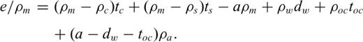
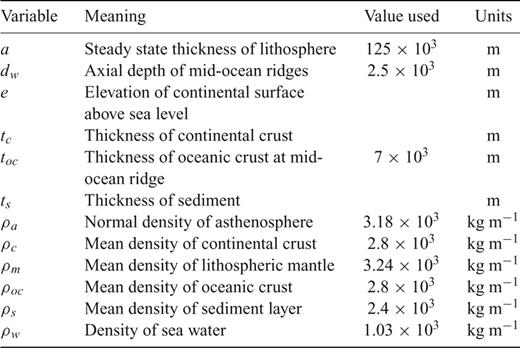
Variables used in isostatic balance.

Open in new tabDownload slide

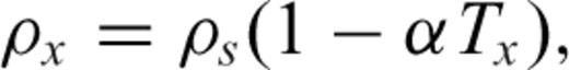
First, Moho depths from Fig. 11 were converted into average crustal thicknesses. Where necessary, sedimentary thickness was taken into account (Divins 2008). Elevation, e, was then calculated using mean values of crust and mantle densities, which were estimated by assuming a linear temperature dependence with depth (Bown 1993). Subtracting expected elevation from filtered topography yields residual topography. It is important to filter topography so that wavelengths shorter than 100–200 km are removed. At the shortest wavelengths, isostatic compensation breaks down due to the finite flexural rigidity of the lithosphere (Tiley et al. 2003). Negative topography (i.e. bathymetry) is converted into an air-loaded form by multiplying it by 0.7. In this way, a gridded and smoothed map of residual topography was generated (Smith & Wessel 1990; Fig. 12).

Figure 12

Map of residual topography calculated by isostatically balancing crust and lithosphere at each sample point against a mid-oceanic ridge. Greatest difference between calculated and observed elevation occurs in northwest Scotland.

Open in new tabDownload slide

Residual topography increases towards the northwest of the British Isles and values as high as ∼1 km occur beneath northwest Scotland and northwest Ireland and their coastal shelves. Further south, residual topography is generally less than ±300 m and can be regarded as negligible given the uncertainty in relating crustal velocity and density. It is well-known that northern Britain is not isostatically compensated and there is evidence for vertical uplift as a result of postglacial rebound. Bradley et al. (2009) analysed uplift velocities from continuous global positioning system (CGPS) measurements across Britain. In Scotland, they find that surface elevation is rising by ∼1 mm yr⁻¹. The surface elevation of England is decreasing at a similar rate. This differential movement is attributed to postglacial isostatic adjustment. However, postglacial rebound cannot account for either the sign or amplitude of residual topography in northwest Scotland.

Postglacial rebound acts to restore the Earth's surface to its elevation before an ice load is imposed. CGPS measurements in Scotland indicate that rebound is still occurring, which suggests that the state of equilibrium which existed prior to loading has not yet been restored. However, nearly 1 km of residual topography exists which must therefore be a minimum since postglacial rebound is not complete. Away from Scotland, the amplitude of residual topography is much smaller and it is difficult to disentangle pre- and postglacial displacements. For example, negative residual topography in north Wales could easily result from incomplete postglacial rebound (Lambeck 1993).

It is important to bear in mind that crustal density variations can support residual topography. Positive residual topography of northwestern Scotland could, in part, arise from a regional reduction in crustal density. For example, at BOHN, a 10 percent density reduction could account for its elevation. Nonetheless, the surface outcrop of northwest Scotland is not consistent with a wholesale density decrease. Local variations in crustal density are expected, but they cannot account for largest amplitude of residual topography. It is also possible to produce residual topography by reducing lithospheric density. For example, gabbroic sills could have been intruded into the sub-Moho mantle beneath the western seaboard of Scotland at depths of ∼40 km (Maclennan & Lovell 2002). This low density material could provide additional isostatic support, which is not taken into account by our residual depth analysis. Immediately north of Scotland, a grid of deep reflection and wide-angle profiles occur (e.g. DRUM, ORKNEY-92 profiles; Flack & Warner 1990; Price & Morgan 2000). In this area, we estimate that there is ∼900 m of positive residual topography. To account for this amplitude requires a gabbroic layer >10 km thick, assuming a density of 2.9 Mg m⁻³. The thickness and density of this layer indicate that it should be detectable by controlled-source experiments but no mantle velocity anomaly beneath the Moho between 26 and 40 km depths has been reported.

Residual topography in northwest Scotland is consistent with a decrease in asthenospheric mantle density, possibly as a result of an increase in mantle temperature. In the North Atlantic Ocean, there is excellent evidence which shows that anomalously shallow oceanic lithosphere surrounds the Icelandic plume, a region of convective upwelling (White 1988). The decrease in density from the rising hot material causes a buoyancy effect which supports the oceanic plate. Using admittance calculations, Jones et al. (2002) calculated the peak support at Iceland to be around 2 km, reducing to 500 m towards the continental shelf. Converting their water-loaded value to an air-load yields ∼700 m. Similarly, Tiley et al. (2003) noted a departure between observed and calculated admittance at the longest wavelengths (400–1000 km) for the British Isles. They attributed this departure to convective dynamic support, although their calculations cannot localize this uplift since they were carried out in the frequency domain.

If uplift is caused by a patch of anomalous asthenospheric density, the decrease in density for a given layer thickness and the consequent temperature increase can be estimated. The density of this layer, ρ_x, is calculated by isostatically balancing against a normal asthenospheric mantle profile. Next, the expected temperature, T_x, giving rise to the decrease in density may be estimated using

5

where the density of mantle at standard temperature and pressure, ρ_s, is 3.33 × 10³ kg m⁻³ and the thermal expansion coefficient of the matrix, α, is 3.4 × 10⁻⁵°C⁻¹ (Bown 1993). For a conservative value of 500 m of uplift and a layer thickness of 100 km, the increase in temperature is approximately 135°C. This value is similar to that calculated by Rudge et al. (2008) to account for uplift events north of Scotland at ∼55 Ma.

A variety of regional tomographic models suggest that the asthenospheric mantle beneath northwest Britain is anomalously slow and possibly hot. The P-wave velocity models of Bijwaard et al. (1998) and Arrowsmith et al. (2005), as well as the earlier S-wave velocity model of Marquering & Snieder (1996) reveal slow subplate velocities beneath the British Isles. Some surface wave tomographic models suggest that anomalously slow velocities occur beneath this region (Schivardi & Morelli 2009). Finally, a full waveform inversion of upper mantle structure beneath Europe indicates that there is a patch of anomalously slow velocity centred beneath the Irish Sea at 100 km depth (Fichtner & Trampert 2011). Goes et al. (2000) converted earlier models into temperature values, which suggests that there is an increase of up to 200°C above normal asthenospheric temperatures at subplate depths. Bott & Bott (2004) used these results to suggest that Cenozoic uplift of the British Isles is generated by localized convective upwelling of hot asthenosphere. Our results imply that the temperature of this anomaly could be reduced, which is significant because it is important that the geothermal gradient beneath the plate does not overstep the dry peridotite solidus.

5 Conclusions

We have carried out a detailed receiver function study of the British Isles. 39 stacked receiver functions show clear arrivals from the Moho discontinuity and from intracrustal interfaces. H−κ plots suggest that the crust is ∼30.4 km depth with an average V_p/V_s ratio of 1.74. A combination of careful forward and inverse modelling was then carried out to determine the detailed velocity structure at each station. These results bear out the preliminary analysis and are in excellent agreement with legacy controlled-source experiments.

Our most important conclusion is that crustal thickness decreases northwards. This decrease negatively correlates with average elevation and it is difficult to explain by changes in crustal density alone. Instead, we suggest that sublithospheric isostatic support occurs which may be generated by a warm tongue of asthenosphere protruding southwards from the Icelandic plume. The existence of anomalous asthenosphere is supported by the spectral relationship between free-air gravity anomalies and topography and by regional tomographic studies. A secondary conclusion is that a thick layer of fast lower crustal rocks occurs beneath Scotland and extends southwards. The position of this layer broadly correlates with the surficial trace of Cenozoic magmatism and with the location of Palaeogene denudation. These observations are consistent with, but do not prove, the hypothesis of magmatic underplating.

The present-day crustal structure of the British Isles supports the notion that vertical movements during Cenozoic times are predominantly controlled by epeirogeny associated with the Icelandic plume. While there is copious field evidence for phases of horizontal shortening during Cenozoic times, the magnitude of shortening is one order of magnitude smaller than required. Furthermore, the spatial distribution of upper crustal shortening poorly correlates with the pattern of denudation.

6 Acknowledgments

We thank Isle of Man Astronomical Society, Long Mynd Gliding Club, Mullard Radio Astronomy Observatory, D. Patterson, K. Smith and M. White for hosting seismometer deployments. AWE-Blacknest, BGS, DIAS, GEOFON, IRIS, NEAT and ORFEUS generously provided additional seismograms. We thank I. Frame, D. Lyness, M. Shaw Champion, G. Roberts, K. Sheen and J. Winterbourne for their assistance. Two reviewers helped us to improve and streamline the manuscript. Figures were prepared using the Generic Mapping Tools of Wessel & Smith (1998). Department of Earth Sciences contribution number esc.2432.

Appendix

Figure A1

Velocity models for stations ABER—HPK. Black line: mean receiver function within selected back-azimuthal range. Blue lines – input velocity model fitted by eye and corresponding receiver function. Red lines – average output of best 50 velocity models from Monte Carlo scheme and corresponding receiver function. Grey envelopes – 1 standard deviation of best 50 velocity models and 1 standard deviation of receiver function data. Velocity models for stations PGB—WTSB.

Open in new tabDownload slide

Figure A2

Uninterpreted H−κ stack plots for stations ABER—KESW. Warm colours indicate high amplitudes, according to scale bar. Thin black lines – contours drawn every 0.04. Uninterpreted H−κ stack plots for stations KPL—WTSB.

Open in new tabDownload slide

References

Author notes