


Summary
Baffin Bay represents the northern extension of the extinct rift system in the Labrador Sea. While the extent of oceanic crust and magnetic spreading anomalies are well constrained in the Labrador Sea, no magnetic spreading anomalies have yet been identified in Baffin Bay. Thus, the nature and evolution of the Baffin Bay crust remain uncertain. To clearly characterize the crust in southern Baffin Bay, 42 ocean bottom seismographs were deployed along a 710-km-long seismic refraction line, from Baffin Island to Greenland. Multichannel seismic reflection, gravity and magnetic anomaly data were recorded along the same transect. Using forward modelling and inversion of observed traveltimes from dense airgun shots, a P-wave velocity model was obtained. The detailed morphology of the basement was constrained using the seismic reflection data. A 2-D density model supports and complements the P-wave modelling. Sediments of up to 6 km in thickness with P-wave velocities of 1.8–4.0 km s-1 are imaged in the centre of Baffin Bay. Oceanic crust underlies at least 305 km of the profile. The oceanic crust is 7.5 km thick on average and is modelled as three layers. Oceanic layer 2 ranges in P-wave velocity from 4.8 to 6.4 km s-1 and is divided into basalts and dykes. Oceanic layer 3 displays P-wave velocities of 6.4–7.2 km s-1. The Greenland continental crust is up to 25 km thick along the line and divided into an upper, middle and lower crust with P-wave velocities from 5.3 to 7.0 km s-1. The upper and middle continental crust thin over a 120-km-wide continent-ocean transition zone. We classify this margin as a volcanic continental margin as seaward dipping reflectors are imaged from the seismic reflection data and mafic intrusions in the lower crust can be inferred from the seismic refraction data. The profile did not reach continental crust on the Baffin Island margin, which implies a transition zone of 150 km length at most. The new information on the extent of oceanic crust is used with published poles of rotation to develop a new kinematic model of the evolution of oceanic crust in southern Baffin Bay.
1 Introduction
Baffin Bay is located between the Canadian Baffin Island and Greenland. It represents the northern extension of the rift system in the Labrador Sea, from which it is separated by the bathymetric high of Davis Strait (Fig. 1). Although the opening of the Northeast Atlantic is an ongoing process, the opening of the Labrador Sea and Baffin Bay ceased in mid-Eocene times (Chalmers & Pulvertaft 2001). Since then, subsidence and sedimentation are the dominant geologic processes in these basins.
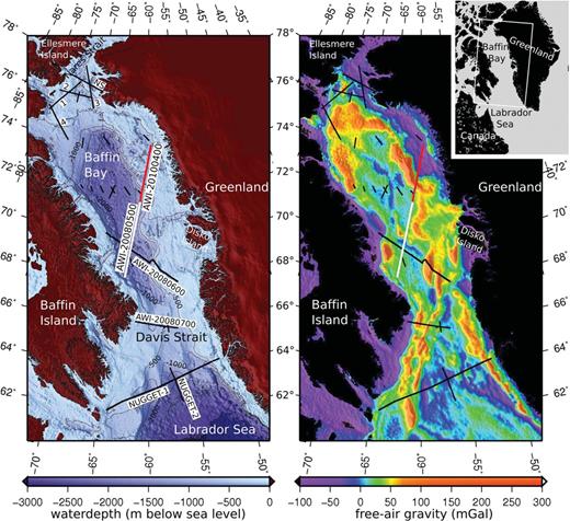
Left-hand panel: bathymetric map of the Baffin Bay area (GEBCO_08 Grid, Version 20090202, ) with place names and locations of published seismic refraction data. The profiles discussed in this paper are marked in white and red (Gohl 2009; Damm 2010), short black lines mark sonobuoy profiles from Keen & Barrett (1972); all other data are seismic refraction lines; Numbers 1-4 are line 1-4 (Jackson & Reid 1994; Reid & Jackson 1997); NS is Nares Strait Line 3 (Funck 2006); AWI-20080600 (Funck 2012; submitted); AWI-20080700 (Gohl et al. 2009; in preparation); NUGGET-1 and -2 (Funck 2007; Gerlings 2009). Right-hand panel: free-air gravity anomalies derived from satellite altimetry (Sandwell & Smith 2009; version 18.1) of the offshore area of Baffin Bay. The same locations as in the left map are marked.
The crustal structure and evolution of the Labrador Sea have been studied in detail (Chian & Louden 1994; Chalmers & Pulvertaft 2001). Magnetic spreading anomalies can clearly be identified in the central Labrador Sea and models of oceanic spreading have been proposed (Srivastava 1978; Roest & Srivastava 1989; Oakey 2005). However, the identification of the oldest magnetic spreading anomaly remains enigmatic. Roest & Srivastava (1989) use chron 33 in their model, which dates to 74-82 Ma after Gradstein (2004), while Chalmers & Laursen (1995) argue that magnetic anomaly 27 N is the oldest one observed, 62 Ma after Gradstein (2004).
The extent of oceanic, transitional and continental crust in the northern Labrador Sea has been mapped with two seismic refraction lines (Funck 2007; Gerlings 2009). Along NUGGET line 1 a 140-km-long segment of oceanic crust is interpreted between continental blocks (Funck 2007). A layer of magmatic underplating is modelled beneath the oceanic crust and for 200 km at the Greenland margin (Funck 2007). NUGGET line 2 images the transition from continental to oceanic crust (Gerlings 2009).
Although the evolution of Baffin Bay is closely related to the evolution of the Labrador Sea, no clear magnetic spreading anomalies are identified there. Therefore, the nature and evolution of oceanic crust in Baffin Bay remain uncertain.
A first comprehensive study on the nature of Baffin Bay crust is provided by Keen & Barrett (1972). From sonobuoy recordings, the crust of the central basin is interpreted as abnormally thin oceanic crust. Rice & Shade (1982) and Jackson (1992) identify oceanic crust in northern Baffin Bay from seismic reflection lines.
In northern Baffin Bay five seismic refraction lines are located near Ellesmere Island and across Nares Strait (Fig. 1; Jackson & Reid 1994; Reid & Jackson 1997; Funck 2006). Line 1 and 3 image a thinning of crystalline crust towards the basin but no oceanic crust (Jackson & Reid 1994). Along line 4 (Fig. 1) serpentinized mantle is interpreted which implies an amagmatic continental margin (Reid & Jackson 1997).
Mainly from potential field data, Chalmers & Oakey (2007) compiled a tectonic map of the Baffin Bay and Labrador Sea region. This is incorporated in the Geological Map of the Arctic (Harrison 2008), but will be quoted as Chalmers & Oakey (2007) in this study. The locations of extinct spreading centres in Baffin Bay are oriented along distinct free-air gravity lows, striking northwest-southeast, as previously proposed by Chalmers & Pulvertaft (2001) and also visible in Fig. 1. Chalmers & Oakey (2007) differentiate Palaeocene from Eocene oceanic crust due to a change of direction in seafloor spreading.
To clearly characterize the type and extension of the crust in Baffin Bay, we present data from ocean bottom seismographs (OBS) along a 710-km-long seismic refraction line in southern Baffin Bay (Figs 1 and 2). The line is oriented across the proposed location of an extinct spreading centre and oceanic crust of Palaeocene and Eocene age (Chalmers & Oakey 2007). Multichannel seismic reflection (MCS) data are used to model the detailed morphology of the basement. Magnetic field data are analysed for indications of magnetic spreading anomalies and volcanic intrusions. Additional density modelling was performed using shipboard gravity data to complement the P-wave model. This analysis now allows for the characterization of the crustal affinity in southern Baffin Bay. From previous plate reconstruction models (Roest & Srivastava 1989; Oakey 2005; Müller 2008), we chose the poles of rotation from Oakey (2005) and with our new data, develop a kinematic model for the evolution of oceanic crust in southern Baffin Bay.
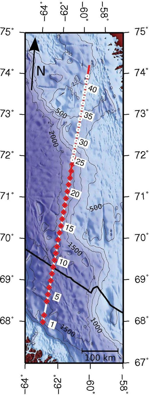
Locations of OBS along line AWI-20080500 (white line with red OBS locations) and AWI-20100400 (red line with white OBS locations); OBS 3 did not record data and is therefore not marked; line AWI-20080600 is marked in black; bathymetry map from GEBCO_08 Grid, Version 20090202,.
2 Tectonic Background of the Opening of the Labrador Sea and Baffin Bay
Baffin Bay and the Labrador Sea formed during Palaeocene to Eocene times when the Greenland Plate first separated from the North American craton and subsequently from Eurasia (Tessensohn & Piepjohn 2000; Chalmers & Pulvertaft 2001). The opening history of Canada and Greenland is derived from magnetic spreading anomalies in the North Atlantic and Labrador Sea by various authors (Srivastava 1978; Roest & Srivastava 1989; Chalmers & Laursen 1995). Srivastava (1978) first dated magnetic spreading anomalies in the Labrador Sea and proposed a single, linear spreading centre in Baffin Bay. Roest & Srivastava (1989) modified the previous reconstruction and suggested two spreading centres in Baffin Bay, separated by a transform fault. Jackson (1992) again proposed a single spreading centre. The latest opening reconstruction from Oakey (2005) uses the isochrones from Roest & Srivastava (1989) in the Labrador Sea and the geometry of fracture zones.
The initiation of extension between Canada and Greenland is dated to 223-150 Ma from dykes in southwest Greenland (Larsen 2009). Following extension, regional rifting emplaced a >400-km long dyke swarm in a coast-parallel fracture system in Southwest Greenland from 140 to 133 Ma (Watt 1969). The duration of rifting is disputed, as the timing of initial breakup remains uncertain. The oldest undisputed magnetic spreading anomaly is chron 27N (Chalmers & Laursen 1995).
The motion of the Greenland Plate relative to the North American Plate changed at magnetic chron 24 from an eastward motion to a more northeastward motion, indicated by the orientation of magnetic spreading anomalies (Srivastava 1978; Roest & Srivastava 1989; Oakey 2005). The breakup between east Greenland and northwest Europe is also dated to chron 24 (Talwani & Eldholm 1977; Olesen 2007) and may thus have caused the change in motion of the Greenland Plate. According to Storey (1998), the reorientation of spreading caused a volcanic pulse at 54.8-53.6 Ma in the Disko Island area. An older volcanic pulse is identified at 60.7-59.4 Ma and correlated with the arrival of the Greenland-Iceland mantle plume (Storey 1998). Spreading ceased in the Labrador Sea between chrons 20 and 13 (Srivastava 1978), while spreading between Greenland and Eurasia and the opening of the Northeast Atlantic is ongoing.
3 Data Acquisition
The seismic and potential field data presented in this study consist of two profiles (Figs 1 and 2), acquired during the research cruise MSM09/3 of RV Maria S. Merian in 2008 (line AWI-20080500, Gohl 2009) and the cruise ARK-XXV/3 of RV Polarstern in 2010 (line AWI-20100400, Damm 2010). While AWI-20080500 and AWI-20100400 denote seismic refraction lines, BGR08-304 and BGR10-309 refer to seismic reflection, gravity and magnetic anomaly data along the same lines. The survey in 2008 was designed to cross the proposed location of an extinct Eocene spreading centre as well as various units of oceanic and transitional crust, according to the tectonic map of Chalmers & Oakey (2007). On the 2010 cruise, the line from 2008 was extended to image the transition from thin crust in the centre of the basin to continental crust on the Greenland shelf.
The 24 southernmost ocean bottom seismometers belong to line AWI-20080500, an additional 17 OBS were deployed along line AWI-20100400. An overlap of 72 km of both profiles was chosen to ensure overlapping ray coverage in the deep crust. Acquisition parameters of both surveys are listed in Table 1. On both seismic refraction lines, MCS data were acquired. Parameters of the MCS setup are summarized in Table 2.
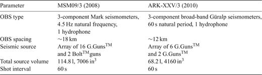
Parameters of seismic refraction measurements.
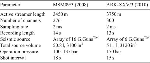
Parameters of MCS measurements.
Gravity data were recorded in 2008 with the KSS31M and in 2010 with the KSS31 sea gravimeters (Bodensee Gravitymeter Geosystem GmbH) at 1 Hz sampling rate. To reference the shipboard gravity data connection measurements were carried out with a LaCoste & Romberg land gravity meter at the beginning and end of each cruise (Gohl 2009; Damm 2010). Magnetic field data were recorded on RV Maria S. Merian with an Overhauser SeaSPY marine magnetometer system towed approximately 600 m behind the vessel. On the Polarstern cruise, an Overhauser SeaSPY marine gradient magnetometer system consisting of two sensors at 150 m distance was used. The use of a gradiometer allows for the elimination of the diurnal variations induced by solar storms during the survey (Roeser 2002). Multibeam bathymetry data were recorded during both cruises. In this study, we only use the centre beam for depth of the seafloor in the P-wave velocity and density models. Research vessel Maria S. Merian is equipped with an EM-120 multibeam echo-sounder for continuous mapping of the seafloor while on research vessel Polarstern, a Hydrosweep DS-2 swath system was operated. For calibration of the depth measurements, sonic log profiles were acquired on both cruises.
4 Seismic Data
4.1 Processing of seismic data
Raw data from the OBS recorders were merged with navigation data, transferred to SEGY-format, cut according to the shot interval into 60 s traces and the OBS locations were more accurately determined using direct arrivals. We picked all refracted and reflected signals with the software ZP (by B. Zelt), using a bandpass filter of 4-15 Hz applied for the near offset signals (±30 km distance from the OBS) and 4-10 Hz for more distant signals. Picking errors of 0.02-0.50 ms were assigned manually for each phase.
In the MCS data, we mapped the basement for the P-wave velocity and density model (Fig. 3). We processed line BGR08-304 with the software package FOCUS™ and line BGR10-309 with ProMAX™. The processing steps are listed in Table 3.
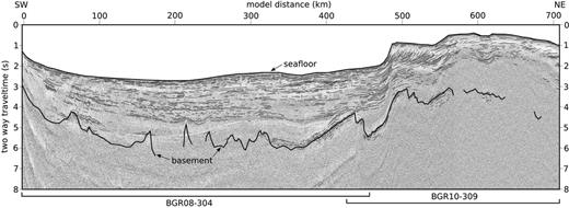
MCS data along line BGR08-304 & BGR10-309 with a line drawing.
Processing of the MCS lines.
4.2 P-wave modelling
We obtained a P-wave velocity structural model with the software RAYINVR (Zelt & Smith 1992) by forward modelling and subsequent inversion of each layer (Figs 4 and A1-A4). The detailed basement morphology was constrained using the high resolution MCS data (Fig. 3). From the model distance of 560-708 km, the depth of basement is modelled with OBS data only, as the basement is not clearly visible on the MCS line. At OBS, 34-41, we modelled deep crustal reflections from water multiples. At OBS 42, a multiple reflection within the sediment cover was used. In areas lacking refracted phases, velocity values were interpolated from constrained velocity nodes nearby.
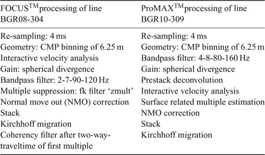
Top panel: magnetic anomaly data along the presented line. Centre panel: P-wave velocity model. White triangles indicate OBS locations; rotated numbers are OBS numbers; numbers on contour lines are P-wave velocities in km s-1; thick layer boundaries mark discontinuities that are constrained by reflections; white shaded areas are not passed by rays. Bottom panel: grid of the diagonal values of the resolution matrix of the P-wave velocity model. Velocity nodes are displayed with black dots and are shifted inside the layers to indicate their affiliation; white triangles indicate OBS locations; rotated numbers are OBS numbers.
Refracted and reflected phases in the sedimentary layers are grouped in the following to Psed and PsedP, respectively. The name of the reflected phase always refers to a reflection at the base of a layer. Beneath the sediments, phases of a layer that we later interpret as basalts are encountered and named Pb and PbP. Apart from the basaltic layer, we divide the crust into three layers: upper crust/dykes (Pc1 and Pc1P), middle crust (Pc2 and Pc2P) and lower crust/oceanic layer 3 (Pc3). Oceanic layer 2 comprises basalt and dyke phases. Reflections from the Moho are named PmP, refractions in the mantle Pn. Phases modelled from multiples in the water column and in the sediment package are identified with superscripts w and s (Figs A1-A4).
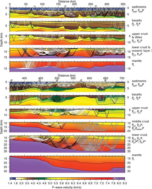
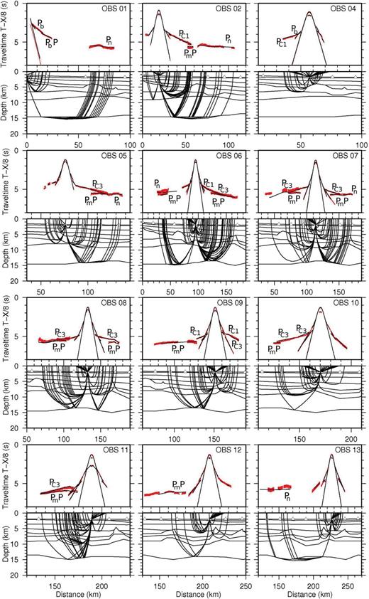
Figs 5 and 6 display sections from different parts of the model where data quality and the corresponding ray tracing were good. In Fig. 5, sediment phases are visible to 16-20 km offset and modelled with a 4-5-km-thick sedimentary cover. Although no Pb or PbP phases are observed in OBS 6, it was necessary to introduce the basalts layer in order to match the basement on the MCS data. The thickness of the basalt layer was determined from the delay required for the crustal phases. OBS 20 does display a Pb phase. Due to the overlay of sediment and crustal phases at the basement, signals from the basaltic layer are often hidden. OBS 6 recorded a strong PmP phase from 30 to 70 km offset. This runs into the Pc3 refraction and coincides with this phase for offsets greater than 50 km. OBS 20 also detected a PmP phase, but it is much weaker and best visible in the multiple at 8 s traveltime. Between offsets -50 to -45 km, a Pn phase was modelled. As there are only few picks for this phase, an accurate determination of the mantle velocity is not possible. In Fig. 6, OBS 29 is displayed as an example for ray tracing in three-layered crust with the refractions Pc1, Pc2 and Pc3. OBS 40 is chosen as an example for modelling from multiples (Fig. 6). The grey dashed rays of the Pc2P and PmP phases are reflected at the seafloor and at the water surface, before propagation in the subsurface. Apart from a Pb phase, these multiples are the only signals at offsets greater than 30 km. A reason for the missing crustal phases can be the absorption of energy by an upper crustal basaltic layer.

Top panel: part of seismic sections from OBS 6 and 20, plotted with a reduction velocity of 8 km s-1 and a bandpass filter of 4-10 Hz. Centre panel: the same sections with picked signals (red bars with bar length according to assigned pick uncertainty) and modelled phases (black lines). Often phases of the lower crust and mantle are stronger in the multiple, as the data from OBS 20 show. Bottom panel: ray tracing in the P-wave velocity model; refracted waves in white, reflected waves in black; for clarity only every fifth ray is drawn; colour scale of the P-wave velocity model according to Fig. 4: blue = water, brown = sediments, green = basalts, orange = dykes, red = oceanic layer 3, purple = mantle; white triangles mark OBS locations.

Top panel: part of seismic sections from OBS 29 and 40, plotted with a reduction velocity of 8 km s-1 and a bandpass filter of 4-10 Hz. Centre panel: the same sections with picked signals (red bars with bar length according to assigned pick uncertainty) and modelled phases (black lines). Bottom panel: ray tracing in the P-wave velocity model; refracted waves in white, reflected waves in black, those derived from the water multiple with grey dashes; for clarity only every fifth ray is drawn; colour scale of the P-wave velocity model according to Fig. 4: blue = water, brown = sediments, green = basalts, yellow = upper crust, orange = middle crust, red = lower crust, purple = mantle; white triangles mark OBS locations.
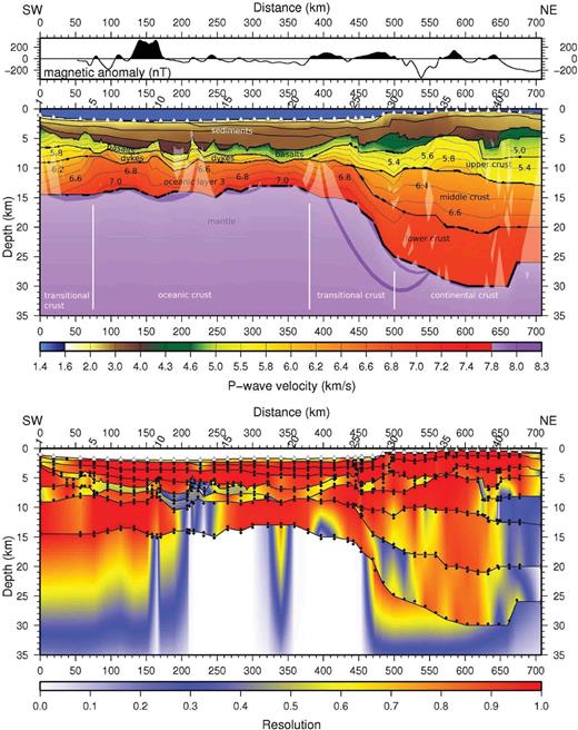
Fig. 7 shows the ray coverage in the different layers to assess how well the model is constrained. P-wave velocities of the sediments are well constrained by refractions with the exception of the lowermost sediment layer between the model distances of 280-420 km. The thickness of this layer is constrained solely by reflections off the basement. The basalts are constrained by Pb and PbP phases for the first 80 km of the model and from a distance of 300 km to the end of the model. In the area between, the layer is needed to model the basement from the MCS data and to account for the delay of other crustal traveltimes. The upper crust and dykes are well constrained by rays between the model distances of 20-170 and 380-620 km. Outside these areas only sparse reflections mark the lower boundary of this layer. The middle crust is mainly modelled from reflections found as multiples. The velocity structure was extrapolated from Pc2 phases at the beginning of the mid-crustal layer (distance 440-520 km). Velocities in the lower crust are well constrained from the model distances of 40-190, 250-380- and 400-480 km. At the Baffin Island margin, the velocities are gradually lowered landward to correspond with the density decrease in the gravity model. On the Greenland margin (distance 480-708 km), the velocity at the top of the lower crust was increased slightly with respect to the middle crust to create a velocity impedance that could generate various Pc2P phases. PmP phases constrain the depth of the Moho along most of the profile. Pn phases are detected for some stations from distance 0 to 320 km. Northeast of the model distance of 320 km, only OBS 36 recorded a mantle refraction (Fig. 7).
Ray coverage of the P-wave velocity model with refracted waves in white, reflected waves in black and rays derived from multiples with grey dashes. For clarity, the model is split in two 355-km-long segments and only every fifth ray is plotted. Each panel displays the phases labelled on the right side.
Table 4 summarizes statistical values as a measure of quality for the model™s fit to the picked traveltimes. The rms traveltime error is calculated by RAYINVR (Zelt & Smith 1992) from the misfit between calculated and picked traveltimes. The normalized Х2 is a measure of how well the calculated traveltimes are within range of the assigned pick uncertainties and should ideally be one. The P-wave velocity model presented here has a normalized Х2 value of 2.3 and an rms traveltime error of 112 ms for modelling without multiples. Typical rms traveltime errors can be in the range of 80 ms (Bullock & Minshull 2005) to 153 ms (Lau 2006). Normalized Х2 values can be higher than 3.7 (Voss 2009), depending on the data quality and assigned pick uncertainty.
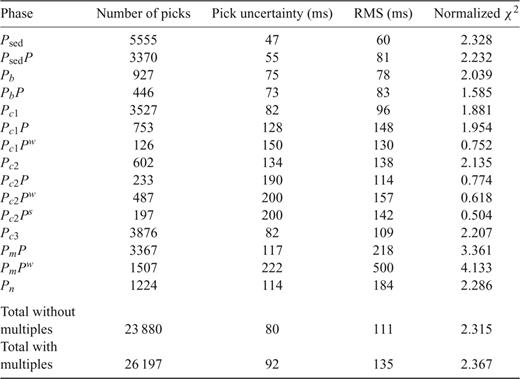
Statistical values of the P-wave velocity model calculated by rayinvr and dmplstsqr for the inversion of each layer. For the inversion of a layer only the rays specifying this layer were activated. Rays from the direct arrival are not taken into account.
Fig. 4 shows the diagonal values of the resolution matrix as a colour grid. These values are calculated at the velocity nodes and provide a measure of how well a velocity value is constrained by all rays passing though it. Lutter & Nowack (1990) refer to values greater than 0.6 as well resolved, which is true for most of the model. Perturbation of single velocity and boundary nodes gives an uncertainty of modelled P-wave velocities and layer thicknesses. The P-wave velocity of the sediment layers and the basalts layer is constrained to ±0.1 km s-1. As the basement is constrained by the MCS data, this boundary can only be varied by ±0.1 km. The P-wave velocities of the upper and middle crust are constrained to ±0.2 km s-1 and their boundaries to ±0.2 km. Where the lower boundary of the middle crust is only modelled from multiples, the uncertainty can reach ±1.0 km. The lower crust is constrained to ±0.1 and ±0.5 km. Where it is modelled from multiples these values can be twice as high.
4.3 Results and interpretation of the P-wave model
The P-wave velocity model (Fig. 4) shows a thick sedimentary layer (up to 6 km) in the centre of the basin from the model distance of 170-200 km. Average velocities of the sediment layers range from 1.8 km s-1 at the top to 4.0 km s-1 at the bottom. The basement morphology varies on the profile from smooth segments in the deep sea environment to fault-block features and rough segments at the Greenland continental shelf (northeast of the model distance of 430 km, Fig. 3). Three distinct basement highs at the distances of 170, 215 and 245 km dominate the basement morphology in the centre of the basin.
The first crustal layer, which we interpret as basalts from the model distance of 0-560 km has velocities ranging from 4.2 to 5.7 km s-1 (Fig. 4). Along the NUGGET line 1 some 600 km to the south, P-wave velocities in the same range (4.2-5.8 km s-1; Funck 2007) were interpreted as basalts and are confirmed by drill holes. Although, there are no drill holes along our line, we adopt this interpretation. The layer we interpret as dykes from the model distance of 0-330 km ranges in velocities from 5.5 to 6.4 km s-1. This interpretation is supported by Gilbert & Salisbury (2011), who report a P-wave velocity range of 5.65-6.61 km s-1 for upper and lower dykes in oceanic crust from samples. From the model distance of 380-708 km, the layer interpreted as upper crust displays velocities of 5.1-6.1 km s-1 and thickens northeastwards. The middle crust is only present from a distance of 440 km northeastwards. The P-wave velocities range from 6.1 to 6.7 km s-1, but are only constrained for the southeastern 80 km by Pc2 phases (Fig. 7). Oceanic layer 3 has P-wave velocities of 6.3-7.2 km s-1 and is 4-7 km thick. P-wave velocities of the lower crust, from distance 520 to 708 km, are modelled with 6.9 km s-1 and 6-10 km thickness. The velocity at the top of the mantle is kept constant at 7.9 km s-1.
The thickness and velocity structure of the crystalline crust, including basalts, upper, middle and lower crust, allow a classification into oceanic, transitional and continental crust.
4.3.1 Oceanic crust
We interpret oceanic crust from model distances of 75-380 km. Due to differences in the oceanic layer 2, comprising basalts and dykes, we separate the oceanic crust into five segments that are described in the following section. Fig. 8 shows vertical velocity profiles of these oceanic sections in comparison with a data review by White (1992). The compiled data by White (1992) represent oceanic crust in the Atlantic, which formed between 59 and 127 ma.
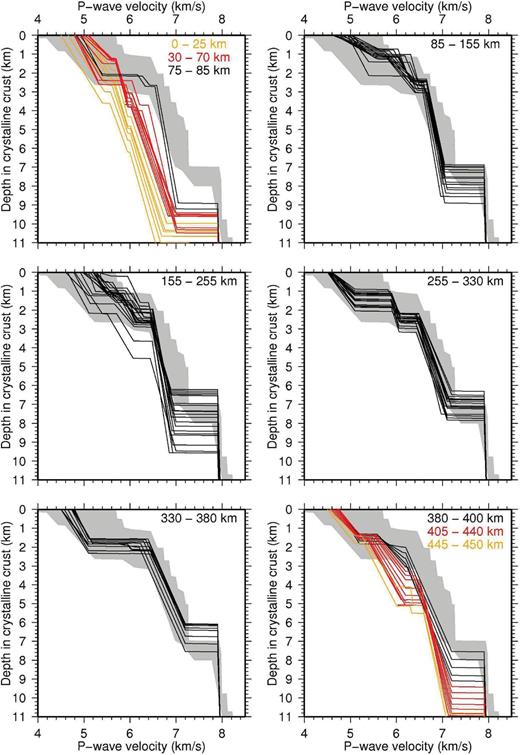
Velocity-depth profiles from different segments of the crystalline crust in the P-wave velocity model, taken every fifth kilometre. Thin black lines are velocity-depth profiles from the model distances labelled in the upper right corner of each panel. Grey shaded is the area outlined by the data compilation from White (1992) of Atlantic oceanic crust from 59 to 127 ma.
- 85-155 and 255-330 km.
The crust is 7-8.5 km thick. Oceanic layer 2 is 1-2.5 km thick and has a P-wave velocity range from 4.8 to 6.4 km s-1. Oceanic layer 3 is 4.5-6.1 km thick with P-wave velocities of 6.4-7.1 km s-1. Fig. 8 shows, that thickness and velocity structure are compatible with oceanic crust.
- 155-255 km.
In the centre of southern Baffin Bay lies the deepest basin along the profile (Fig. 4, from model distance 170-200 km) with basement ridges on both sides. The velocity structure does not vary significantly from the previously described sections. From distance 190 km to 210 km, the crust is only 6 km thick with a thickening of the oceanic layer 3 to both sides. Due to the thinner crust and the deep basin, we propose that this part of the profile represents an extinct spreading centre. Notable is also the symmetry of the Moho topography to this axis. Adjacent to the location of the extinct spreading centre, the crust thickens to 9 km, due to a thickening of oceanic layer 3 by 3 km and ridges in oceanic layer 2. The changes in thickness are well illustrated by the variability of velocity-depth profiles in Fig. 8.
- 75-85 and 330-380 km.
Along the model distance of 330-380 km, the crust is very homogeneous with respect to basement morphology and to thickness (6-7.5 km). In contrast to the previously mentioned segments, oceanic layer 2 is not divided into two layers. The basaltic layer with velocities of 4.7-5.1 km s-1 lies directly on the oceanic layer 3 with velocities of 6.3-7.2 km s-1. The small segment from the model distance of 75-85 km has a crustal thickness of 8.5 km. In oceanic layer 2, the basaltic layer thickens while the layer of dykes thins to only 0.5 km.
4.3.2 Continental crust
500–710 km, Greenland. The crust is 21–23.5 km thick and consists of an upper, middle and lower crust with an additional upper crustal layer landwards from a model distance of 620 km. Velocities of the upper crust average to 5.5 km s-1 and decrease northeastwards. The middle crust is modelled with 6.3–6.7 km s-1 and the lower crust with 6.9 km s-1. Both layers are kept homogeneous in their velocity structure as they are not well constrained by the OBS data. Pc2P phases indicate an impedance contrast at the middle to lower crust boundary, which can also exceed the modelled velocity contrast of 0.2 km s-1, but cannot be quantified due to missing ray coverage. The modelled velocity trend of the crust fits well to the P-wave velocity range that Christensen & Mooney (1995) report for extended continental crust. They report P-wave velocity ranges of 4.7–6.5 km s-1 for upper crust, 6.6–6.8 km s-1 for middle crust and 6.8–7.2 km s-1 for lower crust. The minimum of the global average of 30.5±5.3 km thickness (Christensen & Mooney 1995) exceeds the thickness of 23 km found here by only 2.2 km.
Landward of the model distance of 620 km, a layer with P-wave velocities of 5.0 km s-1 is modelled on top of the upper crust. The lower boundary of this layer is only constrained by one reflection (Figs 4 and 7). The P-wave velocities of this layer can equally be interpreted as basalts or consolidated sediments (Fox 1973; Castagna 1985). As the MCS data do not image the basement on this part of the profile well, no interpretation from the basement morphology can be given.
4.3.3 Transitional crust
We here use the term ‘transitional crust’ where thickness and/or velocity structure of the crystalline crust vary significantly from that of oceanic and stretched continental crust.
380–500 km, Greenland. The crust thickens from 8–21 km. At a model distance of 380 km an upper crustal layer appears with an average P-wave velocity of 5.5 km s-1. It thickens from 0 to 4 km over a distance of 60 km with decreasing P-wave velocities further landward. At the model distance of 440 km, a mid-crustal layer appears, which thickens from 0 to 5 km. Notable is also the rise of P-wave velocities in the lower crust by 0.4 km s-1 northeast of a model distance of 430 km, which is consistent with an increase in mafic content. The MCS data show a basement morphology with block faulting after a model distance of 430 km (Fig. 3) and from the distance of 390–410 km seaward dipping reflectors are imaged (Block 2012).
The comparison with the data compilation from White (1992) in Fig. 8 shows, that the oceanic character of the velocity distribution in the crust is well preserved up to a model distance of 400 km. From distance 405 km northeastwards, the thickening of upper and lower crust lead to a mismatch with the oceanic velocity–depth function from White (1992). Though the type ‘oceanic crust’ can be extended to a model distance of 400 km, we interpret the area southwest of 380 km as clear oceanic crust and the area northeast as transitional crust.
0–75 km, Baffin Island. Towards the Baffin Island shelf, the crystalline crust thickens from 8 to 11 km. Upper and lower crust shift to lower P-wave velocities southwestwards, which is consistent with a decreasing amount of mafic material. Velocity–depth functions from model distances of 0–25 km differ from the compilation of White (1992) due to slow P-wave velocities in the upper crust and thick basalts (Fig. 8). From distance 30–70 km, an increase of P-wave velocities in the upper crust and a decreasing thickness of the basalts are modelled and an oceanic character develops. Unfortunately, this part of the profile is not well covered by the OBS data and will be discussed in connection with the density modelling.
5 Gravity Data
5.1 Processing and modelling of the gravity data
Several processing steps were applied to the gravity data to obtain the free-air gravity anomalies for subsequent modelling (Table 5). The forward modelling of gravity data was accomplished with the software GM-SYS (Northwest Geophysical Associates, Inc.). To set up a starting model, we used the geometry and velocity distribution of the P-wave velocity model. We calculated average P-wave velocities for each layer and converted them to density, according to the data synthesis from Barton (1986). To simplify the model, we combined the three upper sedimentary layers into one density unit (Fig. 9). However, we included a lateral variation from 2140 to 2250 kg m-3 between the model distances of 490–580 km in accordance with the higher average P-wave velocities in this part of the model. To obtain a best fit between modelled and observed free-air gravity anomalies, the density values were inverted while the geometry was kept fixed. The inverted density values differ only slightly from the initial values and all lie within the range from Barton (1986). During modelling, we compared the density and the P-wave model and adjusted layer boundaries in either to obtain an optimal correspondence between both. Generally, the correspondence between the P-wave velocity and density models is excellent, except between the model distances of 200–260 and 440–560 km where the geometry of the layer boundaries had to be changed to reproduce the high observed gravity values. The geometry at the ends of the profile were edited to account for the regional gravity field. The rms difference between the observed and modelled gravity is 2.03 mGal on average with a 6.63 mGal maximum at the distance of 483 km (Fig. 9).
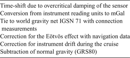
Corrections applied to the gravity data.

Top panel: observed and modelled free-air gravity data (blue and red respectively). Centre panel: difference of modelled and observed gravity. Bottom panel: density model; numbers inside the layers indicate density values in kg m-3.
5.2 Results and interpretation of the density model
The mean free-air gravity value is 24mGal on the first 460 km of the profile (Fig. 9), except for the model distance of 190 km where −mGal were measured. Across the transition to continental crust on the Greenland shelf, the free air gravity rises to 97mGal and then drops to negative values to the northeast with a minimum value of −93mGal.
Along the profile the sediment density varies from 2100 to 2250 kg m−3 on top of a 2350 kg m−3 dense lower sediment layer. The density of the basalts (2500 kg m−3) on oceanic, transitional and continental crust is kept constant, while the other crustal layers vary in density along the profile.
From model distances of 75-430 km the dykes are modelled with 2750 kg m−3. Oceanic layer 3 is modelled by a 2950 kg m−3 dense body, extending from distance 70 to 450 km. From distance 200 to 260 km, the boundary of oceanic layer 2 and 3 differs significantly from the P-wave velocity model. This can represent the actual thickening of the oceanic layer 3 or it can indicate an increase in denser material at this location. As the OBS data do not cover this section well, the density model will be emphasized in the discussion.
The crust of the Baffin Island shelf, from a model distance of 0 to 75 km, is modelled with 2700 and 2800 kg m−3 beneath the basalts. These are lower density values than are needed at the adjacent oceanic crust. The transition to lower densities supports the interpretation of this section as transitional crust, which was already indicated by the P-wave model, but uncertain due to poor ray coverage. The density model already indicates a thickening of the crust to Baffin Island with a deeper Moho at the beginning of the profile. This thickening was not imaged by the OBS data, as the profile was not extended further landward.
From a model distance of 430 km to the northeast, the upper crust is modelled with 2600 kg m−3 and a mid-crustal layer is modelled with 2880 kg m−3 from the distance of 440 km to the end of the model. These values are lower than the densities of the adjacent oceanic layers and thus separate these units. The lower crust displays high density values of 3050 kg m−3, which indicate a mafic composition. Unlike the P-wave model, the density model displays denser middle-crust material at shallower depth at a model distance of 460-530 km. An increase of dense material near the surface is needed to model the distinct higher values of a free-air gravity anomaly at the shelf break. A strong gravity high is observed at various shelf breaks, named ‘sedimentation anomaly’ according to Watts & Fairhead (1999). If a 2-D model is oriented perpendicular to the shelf break, the density contrast between water and sediments is sufficient to model this anomaly. As our line runs oblique to the Greenland shelf (Fig. 1), it is likely, that a 3-D effect of the shelf break leads to the modelled upward arch of dense material in the 2-D model.
6 Magnetic Field Data
On profile BGR08-304, the reference field values of the IGRF-10 were removed from the measured magnetic total intensity values to obtain residual anomaly values. On profile BGR10-309, the reference field IGRF 11 was used. In the overlapping range, the BGR10-309 data were shifted to the BGR08-304 data to obtain a constant anomaly level. Finally, the anomalies on the combined profile were adjusted to meet the mean level of two published magnetic maps (Verhoef 1996; Maus 2009) by adding a constant value of 100 nT.
It was not possible to derive the distribution of oceanic and continental crust from the pattern of the magnetic anomalies alone (Fig. 4). Except for a distinct anomaly around the model distance of 150 km, the oceanic crust is characterized by small amplitudes and shorter wavelengths, while longer wavelengths and higher amplitudes dominate the transitional and continental crust. Despite the thick sediment cover, we had expected to find indications for magnetic spreading anomalies and a distinction for oceanic and continental crust.
7 Plate Kinematic Model
For the plate reconstruction we used GPlates (Boyden 2011; ), which visualizes plate motion on a sphere. We compare published poles of rotation from Roest & Srivastava (1989), Oakey (2005) and the compilation from GPlates (Müller 2008; version 1.0.1). In the reconstruction from GPlates, Baffin Island is moving as a microplate from 95.2 to 33.5 ma. As we did not find any evidence of this, we kept Baffin Island fixed to the North American continent and, therefore, refer to a modified GPlates reconstruction.
The location of extinct spreading centres and the extent of oceanic crust were proposed previously by Srivastava (1978), Roest & Srivastava (1989), Jackson (1992), Tessensohn & Piepjohn (2000), Geoffroy (2001) and Chalmers & Oakey (2007). We digitized the crustal segments from the detailed tectonic map from Chalmers & Oakey (2007) with ArcGIS™ and displayed the evolution of these segments for the different reconstructions to verify the tectonic map.
7.1 Results and interpretation of the plate kinematic model
We rotated the segments of oceanic crust from the tectonic map from Chalmers & Oakey (2007) in GPlates with the rotation poles from Roest & Srivastava (1989), Oakey (2005) and the modified GPlates rotation (Müller 2008). All sets of rotation poles lead to a gap in Palaeocene oceanic crust (Fig. 10). The gap has a maximum width of 44 km for the rotation poles from Oakey (2005), of 57 km for the poles from Roest & Srivastava (1989) and of 88 km for the modified GPlates poles (Müller 2008). This indicates, that either the rotation poles need to be recalculated or that the tectonic map from Chalmers & Oakey (2007) needs modifications. Deriving a new set of rotation poles from our data is not possible but the tectonic map from Chalmers & Oakey (2007) can be modified.
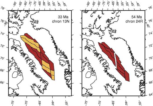
Distribution of oceanic crust from Chalmers & Oakey (2007). Dark brown segments are Palaeocene oceanic crust, light brown segments are Eocene oceanic crust. The configuration at 33 ma (left-hand panel) is also valid for today. At 54 ma (right-hand panel) the greatest gap occurs in Palaeocene oceanic crust with the poles of rotation from Oakey (2005).
To explain the missing oceanic crust in the Palaeocene, we outline the extent of oceanic crust at different stages in the reconstruction from Oakey (2005). To date the rotation poles, that are given in magnetic anomaly chrons, we use the timescale from Gradstein (2004).
On the Greenland shelf, we kept the eastern boundary of oceanic crust as proposed by Chalmers & Oakey (2007), which is within an error of 5 km to the boundary we derived from the P-wave velocity and density models of this study. At the Baffin Island shelf, we used the more detailed continent-ocean boundary (COB) from Skaarup (2006), which was derived from seismic reflection data (Fig. 11). At the location of our profile, we modified the COB from Skaarup (2006) according to our interpretation by placing it 17 km further seawards (at a model distance of 75 km). This is 11 km further landward than the COB proposed by Chalmers & Oakey (2007). The location where we interpret the extinct spreading centre corresponds within 5 km with the location of the southern Eocene spreading centre given by Chalmers & Oakey (2007). We orientate the spreading centre along a pronounced low in the free-air gravity data (Fig. 11). The northern Eocene spreading centre was also placed along a distinct gravity low. No assumptions can be made on the extent of oceanic crust in northern Baffin Bay due to a lack of constraining data. By rotating the Greenland Plate back to its position at 47 and 54 ma, we mapped the extent of oceanic crust, avoiding gaps and overlaps. For the Palaeocene oceanic crust, we introduce a spreading centre by dividing the oceanic crust in two equal parts. This differs from the spreading centre from Chalmers & Oakey (2007), who postulate more oceanic crust on the Baffin Island margin (Fig. 10). As we did not find indications for asymmetric spreading, we preferred a spreading centre that produces equal parts of oceanic crust. An uneven distribution of oceanic crust can be indicated by clear magnetic spreading anomalies, which are not observed here. We introduced three spreading centre segments, as the outline of oceanic crust from Chalmers & Oakey (2007) indicates fracture zones in the centre of the Palaeocene crust.
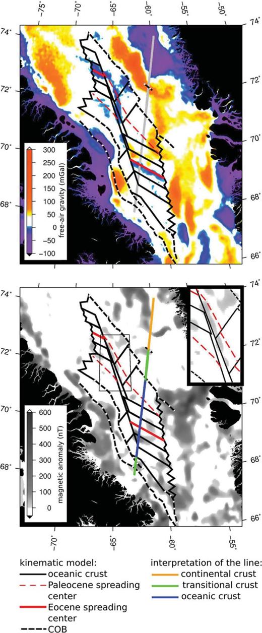
Top panel: features of our kinematic model and the location of the presented line (grey) on top of satellite derived free-air gravity data (Sandwell & Smith 2009; version 18.1). Bottom panel: features of our kinematic model and the location of the presented line with interpretations of the crustal character on top of magnetic anomaly data (EMAG2 V2, Manus et al. 2009). Closeup in the upper right: positive magnetic anomaly at the location of the transform fault.
Fig. 12 illustrates the evolution of oceanic crust in Baffin Bay, according to the results of this study with the rotation poles from Oakey (2005). At 61 ma (chron 26R), oceanic crust begins to form due to east-west extension. At magnetic chron 24N (54 ma) the direction of extension changes to a southeast-northwest direction. This direction change marks the change from Palaeocene to Eocene spreading. The Palaeocene oceanic crust breaks into several fragments as two Eocene spreading centres evolve, connected by a major transform fault. At chron 13N (33 ma), seafloor spreading ceases.
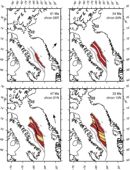
Evolution of oceanic crust in southern Baffin Bay with rotation poles from Oakey (2005). Thick grey lines outline the continent-ocean transition: on the Baffin Island margin from Skaarup (2006), modified at the location of our line; on the Greenland margin from Chalmers & Oakey (2007). The extent of transitional crust is marked on the Greenland margin only at the location of our line. Palaeocene oceanic crust is marked in dark brown, Eocene oceanic crust in light brown, spreading centres in white. Arrows indicate the motion of Greenland relative to the North American Plate.
8 Discussion
8.1 Oceanic crust
Our P-wave and density models show that the basin is mostly underlain by oceanic crust with an average thickness of 7.5 km. Keen & Barrett (1972) report abnormally thin crust of 4 km thickness from sonobuoy readings in the centre of Baffin Bay, along a line at 72°N, 200 km northwest from our line (Fig. 1). We suggest, that the northward decrease in crustal thickness indicates a decrease in magma production.
The oceanic crust in Baffin Bay developed during two stages with different spreading directions (Oakey 2005; Chalmers & Oakey 2007). Our profile is perpendicular to the Eocene spreading centre, which we locate in the P-wave velocity and density model at a model distance of 190-210 km (Figs 4 and 9). From GPlates, the Palaeocene spreading centre is located at a model distance of 300 km (Fig. 12) but we prefer to place it at 292 km (Fig. 13) where a depression is visible in the basement (Figs 4 and 9).
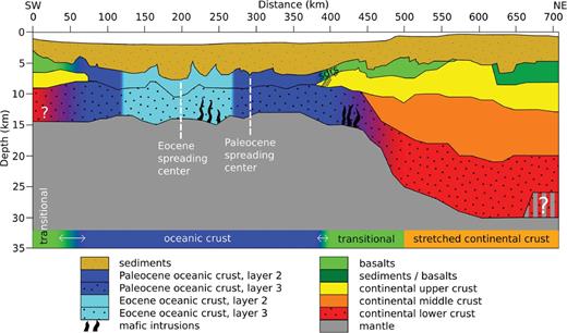
Geologic interpretation of the P-wave and density model.
Oceanic layer 2 consists of basalts and dykes, which are modelled as individual layers. While the basalts layer is always modelled, the dykes were not modelled as a separate layer from a distance of 330-380 km and only as a very thin layer from the model distance of 75-85 km in the P-wave velocity model. These are the regions closest to transitional crust and could indicate a change in material due to spreading or alteration. Where basalts and dykes are modelled as separate layers, only few reflections indicate that there is a significant velocity contrast between them. It is unlikely that oceanic layer 2 does not contain dykes. So where they are not modelled as separate layer, the velocity structure does not allow for discrimination and the velocity contrast between basalts and dykes is more continuous.
In the centre of the basin, north of the extinct Eocene spreading centre, the density model shows a thickening of oceanic layer 3 from the distances of 200-260 km, which is not resolved by the OBS data. This thickening of the lower crust is equivalent to an increase of dense material at this location. The accumulation of dense material and/or the thickening of oceanic layer 3 can be the result of volcanic activity (Jokat & Schmidt-Aursch 2007) or it can represent the natural variability of oceanic crust. As positive free-air gravity anomalies are present 30 km north and south of our line (Fig. 1), the influence of a 3-D effect also needs to be considered.
In the oceanic domain, a symmetric magnetic anomaly pattern around the inferred extinct spreading centre at distances 190-210 km would be expected. Such an anomaly pattern is not observed, neither for the Eocene nor for the Palaeocene spreading. As the oceanic crust in Baffin Bay is highly fragmented, the identification of magnetic spreading anomalies will remain difficult. Fragmentation is caused by the change in spreading direction at magnetic chron 24 (Figs 11 and 12; Srivastava (1978); Roest & Srivastava (1989); Oakey (2005)) and by the offset due to small fractures that accompany spreading.
The high amplitude magnetic anomaly at model distances of 130-170 km remains enigmatic, because neither the P-wave velocity nor the density model indicate a significant difference in material composition. The kinematic model shows that this part of oceanic crust lies at the transition from Palaeocene to Eocene crust and at the southern termination of the major transform fault, linking the northern and southern Eocene spreading centres. The magnetic anomaly data imply, that this region was subject to volcanism, when the spreading direction changed and the transform motion initiated. This region is structurally complex and 3-D effects need to be considered.
8.2 Greenland continental crust
According to the definition from Christensen & Mooney (1995), stretched continental crust is interpreted from a model distance of 500-710 km. On the nearby NUGGET line 1 (Fig. 1), south of Davis Strait, a 10-km-thick layer of P-wave velocities similar to our middle crust is also interpreted as middle crust (6.4-6.6 km s−1) on the Greenland margin (Funck 2007). A 5-km-thick lower layer of 6.6-6.8 km s−1 is interpreted as lower crust (Funck 2007). Although the middle crust velocities are similar in both models, the lower crust velocities differ by 0.2 km s−1. This difference is within the assigned error and as both models are separated by 1100 km along the margin, a variation in composition is not unlikely.
If a greater impedance contrast was modelled between middle and lower crust, for example an average P-wave velocity of 7.3 km s−1 is assumed for the lowest crustal layer, this layer would be 2 km thicker. It would also be interpreted differently, as P-wave velocities higher than 7.2 km s−1 indicate magmatic underplating (White & McKenzie 1989). This interpretation would mean, that middle crust directly overlies an underplated body of 12 km thickness. On the nearby NUGGET line 1 (Fig. 1) a section of the Greenland margin is modelled with an underplated body with a P-wave velocity of 7.4 km s−1 and 5 km thickness below middle crust (Funck 2007). Although the velocity structure is similar, the thickness of the underplating is only one-third. Underplating of 9-16 km thickness is modelled under stretched continental crust on the East Greenland margin, north of the Jan Mayen Fracture Zone along seismic refraction lines (Voss & Jokat 2007). Together with seaward dipping reflector sequences of the initial break-up along 20-50 km distance (Hinz 1987), the profiles are interpreted to indicate a weak-magmatic evolution of the northeastern Greenland margin (Voss 2009). As the P-wave velocity structure of the lower crust is not resolved by the OBS data on our line, an interpretation of stretched continental lower crust with middle crust overlying an underplate is possible.
The Moho has a steep step of 4 km at a model distance of 660-675 km, that was introduced due to PmP phases from three OBS (Figs 7 and A4). The recorded reflections could have also been modelled as an inner crustal reflection. Although the density model also included the steep Moho dip, a flattened boundary would only cause minor changes in the gravity fit. A step of 4 km in the Moho should be isostatically compensated by a depression in the basement, which was not observed. From the available data it cannot be differentiated between a Moho step and an inner crustal reflection.
8.3 Greenland transitional crust
Passive margins are typically characterized as volcanic or magma-poor margins. Ocean-continent transitions of magma-poor margins often display a gradual increase of P-wave velocities from the basement to mantle depth without an abrupt Moho transition due to complete serpentinization of mantle material (Chian & Louden 1994; Reid & Jackson 1997; Minshull 2009). We find PmP phases in the OBS data as well as phases from a layered crust. Therefore, the crust cannot consist completely of serpentinized mantle material. Characteristics of a volcanic margin typically are a high velocity lower crust (magmatic underplating) and seaward dipping reflector sequences of flood basalts, that formed at the initial break-up (Hopper 2003; Mjelde 2005; Voss 2009). Seaward dipping reflectors of flood basalt are imaged on the MCS data from 390 to 410 km (Block 2012), supporting an interpretation as volcanic margin, as does the discussion on magmatic underplating in the previous section.
If the volcanic seaward dipping reflectors found along our line are products of the initial breakup, their counterpart should be found on the Baffin Island margin. According to our kinematic model, these should be located at the Baffin Island coast at 68-68.5°N. Skaarup (2006) mapped seaward dipping reflectors from MCS lines in this area, but do not report any at this location. In the case that no counterpart exists, the Greenland seaward dipping reflectors may be sequences of a later volcanic phase. Studies of the Southeast Greenland margin also report volcanic seaward dipping reflectors on oceanic crust, 180 km seawards of the COB (Hopper 2003). Therefore, seaward dipping reflectors are not necessarily related to the initial break-up.
P-wave velocities in the lower crust rise by 0.3 km s−1 at the model distance of 410-450 km. This can indicate increased mafic composition, as mafic intrusions are often encountered at volcanic margins (Minshull 2009). The density modelling does not require an increase of denser material at this location but this is likely because the density difference is too small to cause a misfit between the observed and calculated gravity values.
8.4 Baffin Island transitional crust
The comparison with velocity-depth profiles from White (1992) shows, that the crust displays oceanic type velocities northeast of a model distance of 30 km (Fig. 8). This is the location, where Skaarup (2006) place the limit of oceanic crust. As the thickness of layers 2 and 3 are not typical according to the compilation from White (1992), we only interpret oceanic crust northeast of 75 km.
The lower crust of the Baffin Island transitional zone has P-wave and density values similar to the middle continental crust of the Greenland side. Regardless of this similarity, it is marked as lower crust in Fig. 13 as it directly overlies the mantle.
A pronounced thickening of crust that would indicate continental crust is not observed, although the profile ends at a distance of 75 km from the Baffin Island coast. The extent of transitional crust can therefore add up to a maximum of 150 km, which is in the same range as the extend of transitional crust at the Greenland margin (120 km).
8.5 Evolution of southern Baffin Bay
We introduce several changes to the tectonic map of Chalmers & Oakey (2007) (Fig. 10). In our kinematic model, we define the extent of oceanic crustal segments differently to prevent gaps in oceanic crust at all times. Based on our P-wave velocity and density model (Figs 4 and 9) we shift the COB at the Baffin Island shelf 11 km westwards, shift the Eocene spreading centre 5 km northwards and reaffirm the extent of transitional crust at the Greenland margin. We shift the Palaeocene spreading centre 20 km southwestwards to obtain equal spreading (Fig. 12). In our kinematic model, the major transform fault, that connects the northern and southern Eocene spreading centres, is rotated by approximately 6° counter-clockwise with respect to the north-south trending transform fault, that Chalmers & Oakey (2007) propose. Chalmers & Oakey (2007) orient the transform fault along a gravity low in the centre of Baffin Bay (Fig. 11). In our model, the transform fault is in the range of the gravity low, but does not fit it exactly. Instead it lies on a positive magnetic anomaly, that has previously been recognized by Oakey (2005) (Fig. 11). We suggest, that the magnetic high is a product of volcanic activity along the major transform fault.
9 Conclusions
We present P-wave velocity and density models along a 710-km long transect in southern Baffin Bay (Figs 4 and 9). With the new information from these models we develop a kinematic model of the evolution of oceanic crust with the rotation poles from Oakey (2005) (Fig. 12).
A minimum of 305 km of oceanic crust of Palaeocene and Eocene age is interpreted from the P-wave velocity and density models. The oceanic crust is 7.5 km thick on average with a sediment package of up to 6 km thickness. From the comparison with Keen & Barrett (1972), we suggest a northward decrease of crustal thickness and therefore of magma production in Baffin Bay. From our models, we are able to propose locations for the extinct Palaeocene and Eocene spreading centres (Fig. 13). Although the profile is oriented along the direction of Eocene spreading, no typical seafloor spreading anomalies are found in the magnetic anomaly data (Fig. 4). Most likely the oceanic crust is too fragmented and covered by too much sediment to display a clear magnetic signature.
On the Greenland shelf, the models image 5 km of sediments on top of a 23-km-thick, three-layered, stretched continental crust (Fig. 13). The Greenland continental margin is classified as a volcanic margin as no evidence of serpentinized mantle material is found and seaward dipping reflectors are imaged on the MCS data (Block 2012). Mafic intrusions in the lower crust are inferred from a P-wave velocity increase and support this interpretation. From the available data, the existence of an underplated body, typical for volcanic margins, is unclear. The crustal structure of the Baffin Island margin is only coarsely resolved by the data presented here as our line did not extent further landward.
Plate kinematic modelling showed that modifications to the tectonic map from Chalmers & Oakey (2007) are necessary. The modified model that we present spans from late Cretaceous to the end of seafloor spreading (Fig. 12). Lows in the free-air gravity data can clearly be attributed to extinct spreading centres (Fig. 11). A distinct high in the magnetic anomaly data can be attributed to a major fracture zone that connects a southern and a northern spreading centre in Baffin Bay in the Eocene (Fig. 11).
Acknowledgments
We thank the masters and crews of RV Maria S. Merian and RV Polarstern for their support during the cruises. We acknowledge the IfM-Geomar for providing the OBS stations to T. Funck via an EU grant in 2008 and the German OBS pool (DEPAS) for providing instruments in 2010. We also thank the German Research Council DFG for funding. Kim Welford and Anke Danowski reviewed the manuscript carefully and offered many helpful comments to improve this paper. We also thank Martin Block and Tabea Altenbernd for their help with the MCS data.
References
Appendix
Appendix A: Ray Tracing in the P-Wave Velocity Model For All Obs
Ray tracing in the P-wave velocity model for OBS 1-13. Top panels: Picked phases in red, with vertical bar length according to the assigned pick uncertainty, calculated traveltimes as thin black lines and phase names. A reduction velocity of 8 km s-1 is used for plotting. Bottom panels: Ray paths of the corresponding phases in the model. For clarity, only every 20th ray is plotted.
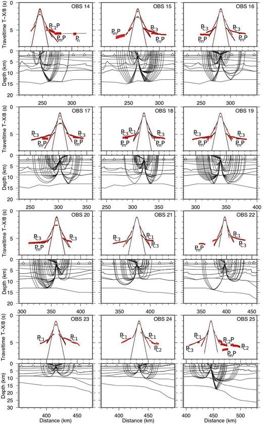
Ray tracing in the P-wave velocity model for OBS 14-25. For the description of the panels see Fig. A1.
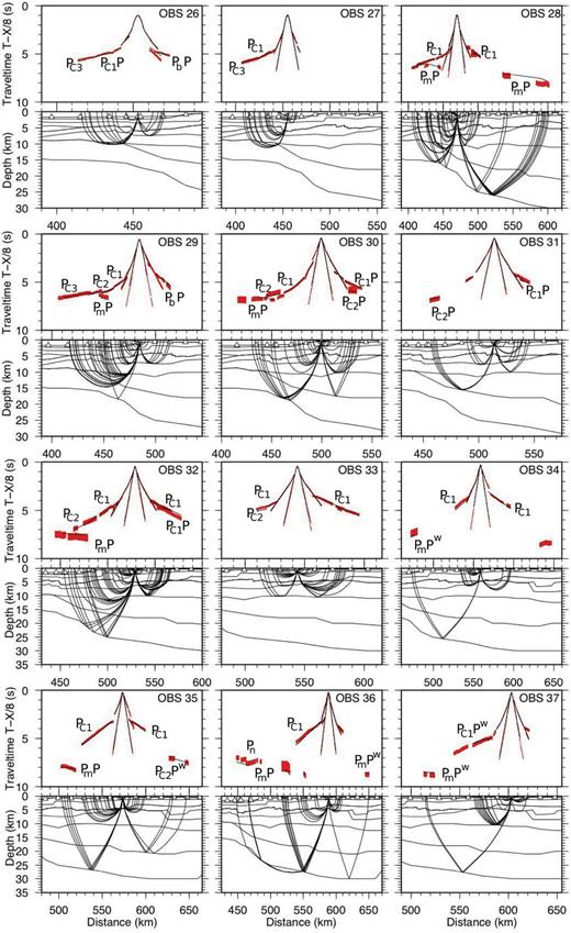
Ray tracing in the P-wave velocity model for OBS 26-37. For the description of the panels see Fig. A1.
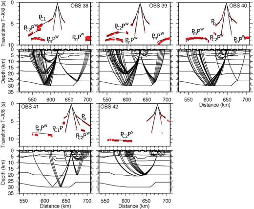
Ray tracing in the P-wave velocity model for OBS 38-42. For the description of the panels see Fig. A1.
