Three-dimensional elastic wave numerical modelling in the presence of surface topography by a collocated-grid finite-difference method on curvilinear grids

Summary

1 Introduction

Modelling the propagation of seismic waves in a complex three-dimensional (3-D) Earth is a fundamental, though difficult, subject in Seismology. Thanks to revolutionary developments in computing technology, such modelling nowadays can be archived by numerical computation. Commonly used numerical methods in seismic wave modelling include: boundary methods that employ Green functions to reduce the problem to the boundaries, and volumetric methods that numerically solve the differential or integral form of the elastodynamic equations for a 3-D grid. Boundary methods, such as the boundary-integral method (BIM) (e.g. Zhou & Chen 2008), and the boundary-element method (BEM) (e.g. Ge & Chen 2007), are very accurate for problems of complex geometry, but are limited to structures only consisting of homogeneous blocks due to the use of the analytical Green functions. Volumetric methods are well suited to complex heterogeneous structures. The finite-difference method (FDM) (e.g. Virieux 1984; Bayliss 1986; Zahradnik 1995; Graves 1996; Moczo 2002; Zhang & Chen 2006; Moczo 2007) and the pseudospectral method (PSM) (e.g. Fornberg 1988, 1990; Tessmer 1992; Tessmer & Kosloff 1994; Wang 2001; Zeng & Liu 2004; Klin 2010) are volumetric methods based on the differential form equations and usually require a structured grid in which each cell can be addressed by an index (i,j,k). The direction of the grid lines of a structured grid could align with the Cartesian coordinate axes with uniform grid spacings (a Cartesian grid) or non-uniform grid spacings (a rectilinear grid), or change point to point (a curvilinear grid). Though an unstructured grid could be used in FDM, it has a lower accuracy and is not widely used (Kaser 2001). One of the advantages of FDM is that it does not require the grid to align with internal discontinuous interfaces (Moczo 2002; Lisitsa 2010), which greatly reduces the difficuties of grid generation and may obviate the need to regenerate the grid if the interfaces change during the structural inversion. Volumetric methods based on integral or variational form of the equations include the finite-volume method (FVM) (e.g. Benjemaa 2007; Brossier 2008), the finite-element method (FEM) (e.g. Bao 1998; Aagaard 2001; Zhang 2007), the spectral-element method (SEM) (e.g. Seriani & Priolo 1994; Faccioli 1997; Komatitsch & Vilotte 1998; Komatitsch & Tromp 1999; Cohen 2002; Chaljub 2007), which is a high-order FEM using orthogonal Chebyshev or Legendre polynomial as the basis function, and the discontinuous-Galerkin method (DG) (Etienne 2010) and the arbitrary high-order derivatives discontinuous-Galerkin method (ADER-DG) (Kaser & Dumbser 2006; Dumbser & Kaser 2006), which are also high-order FEM but use numerical fluxes instead of the basis functions to connect elements. Methods based on the variational form of the equations usually adopt an unstructured grid (tetrahedral or hexahedral grid) and generally deal with the complex geometry more easily if an appropriate unstructured grid has been provided. However, the accuracy of such methods strongly relies on the alignment of the grid and the discontinuous interfaces (Cohen 2002; Pelties 2010), which makes the grid difficult to automatically generate, and indeed the grid may need to completely regenerate during the model inversion if the interfaces change. Professional grid-generation software is usually required to generate high-quality grids. Since each method has its own advantages and disadvantages, hybrid methods are proposed to combine the advantages of different methods (e.g. Moczo 1997; Galis 2008; Goto 2010; Liu 2011).

Due to easy implementation and robustness, FDMs have been widely used in studies of: waveform characteristics in complex structures (e.g. Saenger 2007), strong ground motion (e.g. Olsen & Archuleta 1996; Zhang 2008; Chaljub 2010), the rupture dynamics of earthquake sources (e.g. Cruz-Atienza & Virieux 2004; Cruz-Atienza 2007), wave-equation tomography or full waveform inversion in exploration geophysics (e.g. Luo & Schuster 1991; Pratt & Shipp 1999; Sheng 2006; Virieux & Operto 2009) and finite-frequency tomography in earthquake seismology (e.g. Chen 2007).

Recently, ongoing developments in seismic wave FDM modelling have included high-accuracy and optimal schemes (e.g. Geller & Takeuchi 1998; Berland 2007; Liu & Sen 2009; JafarGandomi & Takenaka 2009), increasing computational efficiencies through the use of non-uniform grid (e.g. Oprsal & Zahradnik 1999; Pitarka 1999), discontinuous grid (e.g. Aoi & Fujiwara 1999; Kristek 2010; Petersson & Sjogreen 2010), subgridding or adaptive mesh refinement (AMR) techniques (e.g. Berger & Oliger 1984; MacNeice 2000; Henshaw & Schwendeman 2008; Kramer 2009), anisotropic media (e.g. Igel 1995; Gao & Zhang 2006; Hestholm 2009; Zhu 2009), spherical coordinates (e.g. Igel 2002; Jahnke 2008; Zhang 2012) and complex geometry (e.g. Wang & Liu 2007; Kaul 2009), especially with surface topography (e.g. Hestholm & Ruud 2002; Hestholm 2003; Zhang & Chen 2006; Ely 2008; Lombard 2008; Appelo & Petersson 2009; Lan & Zhang 2011).

In the FDM framework, there are two strategies to deal with surface topography in terms of the grid: one is to use a Cartesian grid in conjunction with a stair-case approximation of the surface (e.g. Pitarka & Irikura 1996; Robertsson 1996; Ohminato & Chouet 1997; Oprsal & Zahradnik 1999; Perez-Ruiz 2005) or the embedded-boundary method (also called immersed-interface method) (e.g. Kreiss & Petersson 2006; Lombard 2008; Li 2010; AlMuhaidib 2011; Zhang & Zhang 2012), the other is to use curvilinear grids that can conform to the surface topography (e.g. Zhang & Chen 2006; Appelo & Petersson 2009).

The advantages of the Cartesian grids include: the ease of grid generation, the simplicity of the equation to solve and therefore the computational efficiency in the whole-space model or half-space model with a flat free surface and the nature of a center-staggered finite-difference routine that enables it to be used without additional filtering or damping. However, the treatment of topography in Cartesian grids is not trivial. If a stair-case grid to approximate the topography, it will require at least 25 points per wavelength (PPW) if the stress-image technique (Levander 1988; Graves 1996) is used (Ohminato & Chouet 1997) or 60 PPW to achieve good accuracy for Rayleigh waves if the vacuum formulation (Zahradnik 1993; Graves 1996) is applied (Bohlen & Saenger 2006). The embedded-boundary method can avoid spurious diffractions caused by the stair-case approximation. Nevertheless, the application in 3-D and with strong heterogeneities near the free surface may need further investigation.

Curvilinear grids can align with the surface topography and naturally avoid spurious diffractions. In the past, it was thought that FDM for seismic wave modelling could be only used with Cartesian or rectilinear grids, partially because: (i) the widespread staggered FDM requires a rectilinear grid, and (ii) lack of a stable free-surface boundary condition implementation on curvilinear grids. Recent advances in FDM have overcome these problems. Some collocated schemes (also called non-staggered or unstaggered schemes) (Zhang & Chen 2006; Kaul 2009; Tarrass 2011), partly staggered schemes (Ely 2008) and schemes for second-order systems (Appelo & Petersson 2009; Lan & Zhang 2011) have been successfully used to simulate seismic wave propagation on curvilinear grids. Stable free-surface boundary condition implementations on curvilinear grids have been proposed in the second-order system (Appelo & Petersson 2009) for 3-D and in the first-order hyperbolic system for 2-D (Zhang & Chen 2006).

In this study, we extend the 2-D algorithm of Zhang & Chen (2006), which consists of curvilinear grids, a collocated FD scheme and the traction image free surface implementation, to 3-D problems. To begin with, we describe the velocity-stress first-order partial differential equations and the collocated FD scheme for Cartesian grids. Then, the curvilinear grid and first-order hyperbolic equations in curvilinear coordinates are introduced. Also, the traction image method used to implement the free-surface boundary condition on a curvilinear grid is derived. Finally, we use three numerical tests to verify the proposed algorithm.

2 Velocity-Stress Equation and Collocated-Grid Drp/Opt Maccormack Scheme

In 3-D inhomogeneous isotropic elastic media, the propagation of elastic waves is governed by the momentum equation

(1)

and the generalized stress–strain relationship

(2)

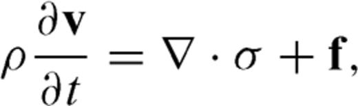
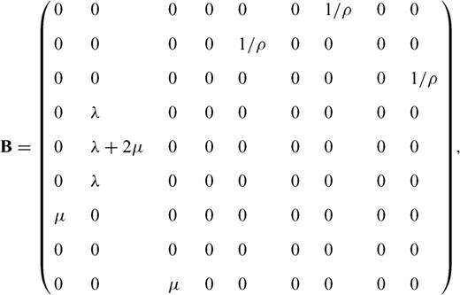
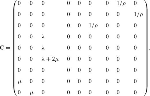
where v=(v_x, v_y, v_z) is the particle velocity vector, is the stress tensor, the components of which are σ_ij, i, j∈ (x, y, z), ρ is the mass density, c is the fourth-order elastic tensor, is the moment density, over which the dot means the time derivative and the superscript T represents the transpose operator.

In the Cartesian coordinates, we can write the first-order velocity-stress hyperbolic system (eqs 1–2) in a compact matrix form:

(3)

where U is the velocity-stress vector

(4)

F is the source vecto

(5)

and coefficients matrices A, B and C are

(6)

(7)

(8)

In these equations, γ and µ are the Lame parameters of the isotropic elastic media.

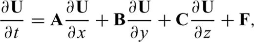
The velocity-stress equations for the isotropic medium in Cartesian coordinates have the elegant property that different components of the velocity-stress vector can be appropriately defined at different half or regular positions in a grid cell in such a way that the spatial derivatives in eq. (3) are only needed half-way between the defined positions of the differentiated variable. Consequently, the simple staggered central difference can be used without the odd-even decoupling problem occurring. Because of its simplicity and robustness, the staggered-grid FDM has been widely used in seismic wave modelling with a flat free surface assumption (e.g. Madariaga 1976; Virieux 1984, 1986; Levander 1988; Rodrigues 1993; Graves 1996; Olsen & Archuleta 1996; Gottschammer & Olsen 2001; Kristek 2002; Moczo 2004).

However, when applied to general anisotropic media or on curvilinear grids, the staggered-grid FDM requires complex interpolations to calculate the quantities needed at positions that are irregularly spaced with respect to the defined locations. Thus, there is a decrease in the overall accuracy (Magnier 1994; Igel 1995). This problem led to the development of the partly staggered grid scheme (Moczo 2007), for example the so-called 3-D grid method (Zhang 1997; Zhang & Liu 2002), the rotated staggered-grid FDM (Saenger 2000), the support-operator method (Ely 2008) and the Lebedev method (Lisitsa & Vishnevskiy 2010), in which all the velocity components are located at the same grid position, while all the stress components share other grid positions.

An alternative choice locates all the components of the particle velocity and stress-tensor at the same grid position, which leads to collocated-grid schemes (also known as non-staggered- or unstaggered-grid schemes). Collocated-grid schemes are well suited to curvilinear grids for problems with complex geometries. However, in comparison with the staggered-grid centre difference, a collocated-grid centre difference has two drawbacks: it has a larger truncation error coefficient (Fornberg 1990) and it has the odd-even decoupling mode (grid-to-grid oscillation, zigzag in 1-D, checkerboard in 2-D) (Patankar 1980, pp. 115–117). To overcome the larger truncation coefficient problem, we could use higher order schemes or high-accuracy schemes like the compact scheme (e.g. Lele 1992) and optimized schemes (e.g. Tam & Webb 1993; Geller & Takeuchi 1998; Zingg 2000; Berland 2007). To avoid the odd-even decoupling that can cause instability, a collocated-grid central difference needs an explicit filtering operation or explicit or inherent dissipation (artificial damping).

One popular and well-tested collocated-grid scheme is the MacCormack-type scheme. The original MacCormack scheme (MacCormack 1969) is second-order accurate in both time and space, and was extended to second-order accuracy in time and fourth-order accuracy in space by Gottlieb & Turkel (1976). This extension of the MacCormack scheme, known as the 2-4 MacCormack scheme, was introduced into seismic wave modelling by Bayliss (1986) with an operator splitting time integration method. It has since been used in a variety of seismic wave problems (e.g. Xie & Yao 1988; Tsingas 1990; Vafidis 1992; Dai 1995). Hixon (1997) used the dispersion relation preserving (DRP) methodology of Tam & Webb (1993) to optimize the dispersion error of the added central difference, and utilized the same methodology to optimize the dissipation error of the one-sided differences in the MacCormack-type schemes. He named this dispersion and dissipation optimized scheme as the DRP/opt MacCormack scheme, which has been used by Zhang & Chen (2006) to model 2-D seismic waves in the presence of surface topography. In the following, we describe the implementation of the DRP/opt MacCormack scheme for the 3-D elastic wave simulation.

In MacCormack-type schemes, the central spatial difference operator is split into forward and backward one-sided difference operators, which are alternately used in multistage Runge-Kutta time marching schemes. Using derivatives with respect to the x-axis as examples, the forward and backward difference operators of the DRP/opt MacCormack are

(9)

(10)

where L_x represents the spatial difference with respect to the x-axis, the subscript i is the grid index, the superscript F means a forward operator, and the superscript B denotes a backward operator. The coefficients a₋₁=−0.30874, a₀=−0.6326, a₁= 1.2330, a₂=−0.3334 and a₃= 0.04168 are obtained by minimizing the dissipation error at eight points or more per wavelength (Hixon 1997), and have fourth-order accuracy for dispersion error.

If all three directional derivatives in eq. (3) are calculated by the forward operator, we get the following discretized right hand side of eq. (3),

(11)

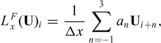
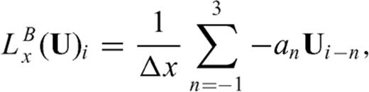
where F or B in the first, second and third subscript65.tif"/> means the forward or backward difference with respect to the x-, y- and z-axes, respectively. We use such syntax, , to represent the discretized right hand side of the equation throughout this paper. In a similar way, we can use the backward difference for all three directional derivatives in 3 and get

(12)

To update the wavefield from time step n to n+ 1, the fourth-order Runge-Kutta scheme evaluates the wavefield at different intermediate times between nΔt and (n+ 1)Δt, and combines the right hand side of eq. (3) at these different times using appropriate weights to get fourth-order accuracy. This can be written as:

(13)

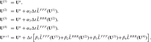
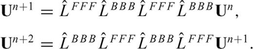
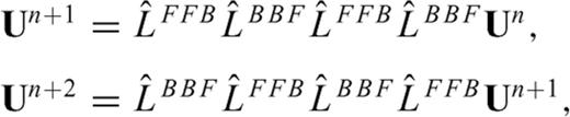
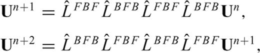
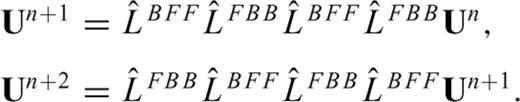
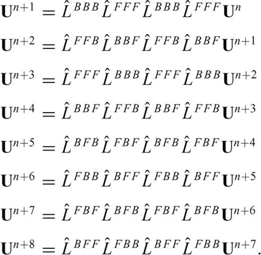
where Uⁿ is the wavefield at time step n, Uⁿ⁺¹ is the wavefield at time step n+ 1 and U⁽¹⁾, U⁽²⁾, U⁽³⁾ and U⁽⁴⁾ are the wavefield at intermediate times nΔt, nΔt+α₂Δt, nΔt+α₃Δt, nΔt+α₄Δt, respectively; the coefficients are α₂= 0.5, α₃= 0.5, α₄= 1, , , and . Note that and are alternately used in eq. (13). The one-sided operators introduce inherent dissipation, which can damp the spurious short-wavelength numerical (or non-physical) waves generated by media discontinuities, computational domain boundaries, grid discontinuities and other computational irregularities, and have a negligible effect on the physical solution. The central difference is recovered when the forward and backward differences are added together at the last step. In this paper, we use the following expression to represent the above fourth-order Runge-Kutta step (eq. 13)

(14)

To avoid numerical bias, the start order of the biased difference operators should be interchanged at every step, resulting in a two-step sequence, which could be written as,

(15)

In actuality, we can mix forward and backward difference operators for the x-, y- and z-derivatives, resulting in three other possible pairs of the 3-D biased difference operators,

(16)

(17)

(18)

We could use two, three or all four pairs of the 3-D MacCormack-type operators, or combine them in many other possible ways. In our experiences, the following combination of all four pairs of operators in an eight time step sequence has better resolution for singularity source terms,

(19)

The stability criterion of the DRP/opt MacCormack with a fourth-order Runge-Kutta scheme is

(20)

in 1-D (Hixon & Turkel 2000) and

(21)

in 3-D, where C_max is the maximum velocity.

3 Surface Topography and Curvilinear Grid

When surface topography is present, we can use curvilinear grids to discretize geological models in such a way that the surface grid layer coincides with the topography (left panel in Fig. 1). Such a curvilinear grid is also called a boundary-conforming or body-fitted grid, as has been used in seismic wave simulations in the pseudospectral (Fornberg 1988; Tessmer 1992; Carcione 1994; Nielsen 1994, 1995) and finite-difference (Hestholm & Ruud 1994, 1998; Zhang & Chen 2006; Wang & Liu 2007; Appelo & Petersson 2009; Lan & Zhang 2011) methods.

Figure 1

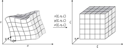
Mapping between (left) the boundary-conforming grid in the physical space (x, y, z) and (right) the uniform grid in the computational space (ξ, η, ζ).

Open in new tabDownload slide

We can map a curvilinear grid in physical space (x, y, z) to a uniform rectangular grid in computational space (ξ, η, ζ), as shown in Fig. 1, through coordinate transformation

(22)

Consequently, the velocity-stress equation (eq. 3) in Cartesian coordinates is also transformed to this computational space using chain rules,

(23)

where the coefficient matrices are

(24)

(25)

(26)

where a comma followed by t, x, y, z, ξ, η and ζ in subscripts means a derivative with respect to the particular variable. For brevity, we use such representations throughout this article. The coordinate mapping coefficients in the above equations can be easily obtained from the Cartesian coordinates of the curvilinear grid points (AppendixA).

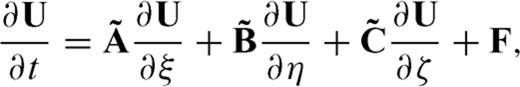
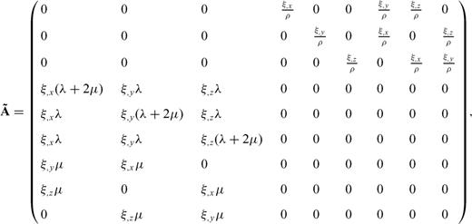
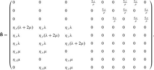
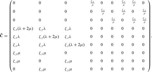
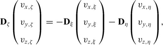
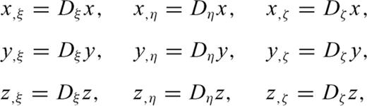
From eqs (23) to (26), we can see that the three directional derivatives of the same variable are required at the same grid position, for example to update v_{x, t}, all σ_{xx, ξ}, σ_{xx, η} and σ_{xx, ζ} are needed. Due to the presence of these derivatives, it is impossible to appropriately stagger the definition of the velocity-stress vector at different positions of a grid cell. However, these extra differential terms from the coordinate mapping do not introduce any problem for the DRP/opt MacCormack scheme, since all the unknowns are defined at the same grid position.

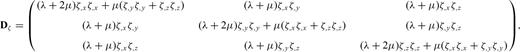
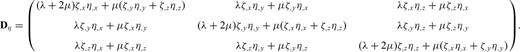
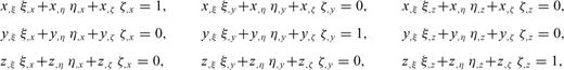
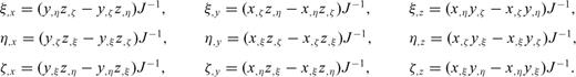
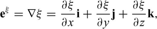
The curvilinear grid sets up a general curvilinear coordinate system (ξ, η, ζ), the base vectors of which vary from point to point. Note that there are two possible definitions of the unknown velocity vector and the stress matrix in a curvilinear coordinate system. One definition is the covariant or contravariant components of the vector and matrix, the directions of which coincide with the local curvilinear coordinate axis. Adopting this definition, we need the Christoffel symbol to account for the derivatives of the component direction (Komatitsch 1996). The other definition continues to use the Cartesian components of the vector and matrix, and only the spatial derivatives are taken with respect to the curvilinear coordinate axes. In this paper, we adopt the second definition that all the unknown are in Cartesian components.

4 Implementation of the Free-Surface Boundary Condition on Curvilinear Grids

The implementation of the free surface is the most difficult part of adopting a collocated-grid finite-difference scheme on curvilinear grids. Due to the lack of implementation of a stable free-surface condition there are rarely any attempts to migrate the many successful collocated-grid finite-difference schemes in computational fluid dynamics and computational aeroacoustics fields to seismic wave simulation. In this section, we propose a stable free-surface boundary implementation on curvilinear grids.

The boundary-conforming grid transforms an irregular surface in physical space (x, y, z) into a ‘flat’surface in computational space (ξ, η, ζ) (Fig. 1). The free-surface boundary conditions will be implemented at this ‘flat’surface.

In the implementation, the ξ−η plane always coincides with the topography. The unit vector perpendicular to the free surface can be easily obtained from the relationship of the covariant and contravariant base vectors of the general curvilinear coordinate (see AppendixB),

(27)

where i, j and k are the unit vectors of the x, y and z-axes in Cartesian coordinates, and .

The free-surface boundary condition requires that the traction T vanishes at the free surface:

(28)

Thus the components of T are zero (substituting eq. 27 into eq. 28),

(29)

(30)

(31)

Since the stress is related to the velocity derivatives through the stress-strain relationship, the above traction component condition also imposes a constraint on the velocity derivatives at the free surface

(32)

where the coefficient matrices are

(33)

(34)

(35)

In a finite-difference scheme based on the first-order velocity-stress hyperbolic system, both the traction condition (eqs 29, 30 and 31) and the velocity derivative condition (eq. 32) should be explicitly satisfied at the free surface.

The difficulty associated with the implementation of the velocity derivative condition (eq. 32) is that it does not provide any symmetric or antisymmetric information for the velocity components, thus the values of the velocity components at the ghost grid points above the free surface are unknown. From the velocity derivative condition (eq. 32), the differential terms with respect to the ζ-axis of the velocity components at the free surface can be calculated from the derivatives with respect to the ξ and η-axis. So, we can update the stress-strain relationship (eq. 2) at the free surface grid layer without knowing the velocity values above the free surface. However, at points several layers below the free surface, updating eq. (2) requires the velocity values at the ghost grid points above the free surface. To set these values, Graves (1996) utilized the zero-stress condition and used a second-order finite-difference expansion of the velocity derivative with respect to the z-axis at the free surface; Robertsson (1996) and Pitarka & Irikura (1996) simply set them to be zero, since the ghost grid points are in the air; Crase (1990) symmetrically imaged these values with respect to the free surface. Another solution is to use a finite-difference operator that does not require the value at the ghost points near the free surface, such as the adjusted finite-difference approximations technique (Kristek 2002), one-sided finite difference (Tarrass 2011) and compact finite-difference scheme (Zhang & Chen 2006). In this paper, we use the following 4/4 compact MacCormack scheme (Hixon & Turkel 2000) for the velocity ζ-derivatives near the free surface:

(36)

(37)

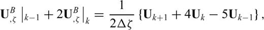
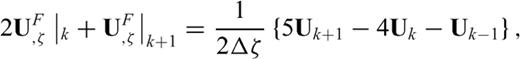
where and denote the forward and backward difference with respect to ζ at grid k, respectively. The merit of this compact scheme is that it uses both the variable's value and its derivative at neighbouring points to calculate the derivative at the current point. Thus, by using only a three-point stencil, it can achieve the same order of accuracy as the explicit scheme in eqs (9)–(10).

To implement the traction-free boundary condition (eqs 29, 30 and 31), we adopt an approach that differs from the common one that sets individual stress component values in the ghost grid points on a flat surface (Levander 1988; Graves 1996). Instead, we antisymmetrically set the traction components in the ghost grid points instead of the stress components, because eqs (29), (30) and (31) imply that the traction components have antisymmetric property with respect to the free surface (suppose the index of the grid layer at the free surface is k₀):

(38)

if we can transform the stress differential terms with respect to the ζ-axis in eq. (1) to traction derivatives, we can calculate these derivatives near the free surface utilizing the antisymmetric traction component values at the ghost points. This can be done by using the conservative form of the ▽ operator (see AppendixC) to rewrite eq. (1) as

(39)

(40)

(41)

where the Jacobian J and the quantity |▽ζ| are non-singular and positive, and can be extended to the ghost points via a symmetric continuation with respect to the free surface. The underlying methodology of this approach is same as the stress image technique (Levander 1988; Graves 1996) for a flat surface, at which traction components are just individual stress components. Our approach is an extension of the stress image to the topographic surface and can be referred to as a traction image technique, which has been used in 2-D seismic wave finite-difference modelling with topography by Zhang & Chen (2006).

Note that the proposed traction image method is not restricted to the DRP/opt MacCormack scheme used in this paper. We chose the DRP/opt MacCormack scheme due to its simple and easy implementation. The traction image method can be used in other collocated grid finite-difference schemes, for example compact schemes and optimal centre difference with explicit filtering schemes.

5 Numerical Verification

In order to verify the collocated-grid finite-difference scheme and the traction image free-surface boundary treatment on curvilinear grids, we present the results of three numerical tests: a homogeneous half-space model with a flat surface, a half-space model covered by a flat layer and a homogeneous model with a 3-D Gaussian hill topography. In these tests, we compare our simulated results of the flat surface model with those from the generalized reflection/transmission coefficients method (GRTM) (Kennett 1983; Luco & Apsel 1983; Chen 1993, 1999), and compare the results of our topographic model with those from the SEM (Faccioli 1997; Komatitsch 1998; Komatitsch & Tromp 1999).

In all the tests, we use a 12-layer-thick ADE CFS-PML (Zhang & Shen 2010) to absorb the out-going waves. The singularity source is approximated by a spatial Gaussian distribution in the curvilinear coordinate system:

(42)

where

(43)

and (ξ₀, η₀, ζ₀) is the source location in the curvilinear coordinate.

5.1 Homogeneous half-space with a flat surface

To verify that the collocated-grid DRP/opt MacCormack scheme can solve the first-order hyperbolic velocity-stress equation on a collocated grid, we perform a numerical simulation in a half-space medium with a flat surface, and compare the simulated displacement seismograms with those derived from GRTM.

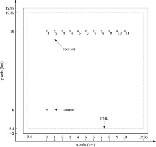
The geometry of the source and the receivers is illustrated in Fig. 2. We use a double-couple source with strike=0°, dip = 45° and rake = 90°, buried 1500 m below the free surface. The source time function is a Ricker wavelet with the centre frequency of 1 Hz. The model and simulation parameters are in Table 1.

Figure 2

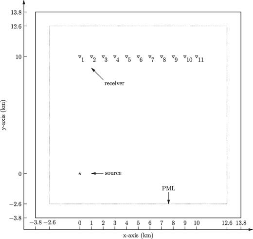
Surface projection of the source-receiver geometry for the half-space with a flat surface. The source (star) is located at (0, 0, −1500 m). There are a total of 11 receivers (triangles) at the free surface, deployed every 1 km from x= 0 to x= 10 km along y= 10 km. The maximum source-receiver distance (at receiver 11) is about 7.0 times the dominant surface wave wavelength and about 17.5 times the minimum surface wave wavelength.

Open in new tabDownload slide

Table 1.

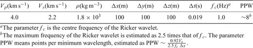
Model and simulation parameters for the half-space model with a flat surface.

Open in new tabDownload slide

To quantitatively assess the agreement in the results of the two methods, in both time and frequency domains, we calculate the time-frequency misfit and goodness-of-fit measurement (Kristekova 2006, 2009a) of the FDM and GRTM solutions. The time-frequency misfit criteria and the goodness-of-fit criteria are calculated from the time-frequency (TF) representation of the signals using a continuous wavelet transform. The benefit of the time-frequency representation is that it can separate the envelope (amplitude) misfit and the phase misfit, and can provide the misfit information simultaneously in both time domain and frequency domains.

The TF goodness-of-fit criteria are most suitable in the case of large differences between two signals (Kristekova 2009a). The misfit criteria for the ‘excellent’level in Kristekova (2009a) are ±0.22 for the envelope misfit, ±0.2 for the phase misfit and 8 for the goodness-of-fit value. All of the comparisons in this study are at the ‘excellent’level. Below, we present time-frequency envelope misfit (TFEM) and phase misfit (TFPM) comparisons. We also show global measurements of the agreement between two solutions: single-valued envelope misfit (EM), phase misfit (PM), envelope goodness-of-fit (EG) and phase goodness-of-fit (PG). All these values are calculated using the TF_MISFIT_GOF_CRITERIA package (Kristekova 2009b).

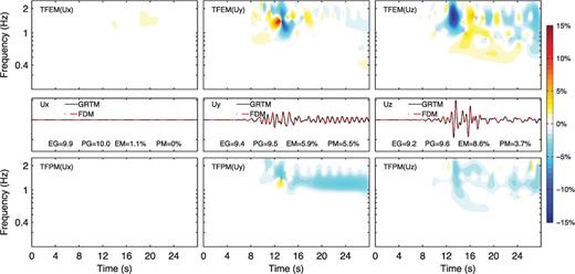
Fig. 3 shows the TF misfit and goodness-of-fit at receiver 1. We can see that the error in the amplitude is relatively larger than the error in the phase, but all the errors over the whole frequency band are below 5 per cent. The DRP/opt MacCormack scheme has inherent dissipation to suspend the odd-even decoupling mode on the collocated grid. This numerical dissipation is the cause of the relative larger error in amplitude than phase. The error is usually greater at higher frequencies, where the wavelength is shorter and there are fewer PPW in the simulation. The largest error happens between 6 and 8 s, where the Rayleigh wave arrives. The Rayleigh wave has shorter horizontal wavelengths and an exponential vertical profile. It requires more PPW than the body-wave phases to achieve the same level of accuracy. Fig. 4 shows the TF misfit and goodness-of-fit at receiver 11. The TFPM and TFEM show similar patterns as in Fig. 3. Due to the Rayleigh wave, the TFEM of the vertical component becomes a little larger (∼9 per cent) at higher frequencies (∼2 Hz).

Figure 3

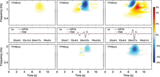
Time-frequency envelope misfit (TFEM; top row) and phase misfit (TFPM, bottom row) between the FDM solutions (dash-dotted red line, middle row) and the reference GRTM solutions (solid black line, middle row) at receiver 1 for the homogeneous half-space model with a flat surface. Left column: x component. Middle column: y component. Right column: z component. Values of the single-valued envelope goodness-of-fit (EG), phase goodness-of-fit (PG), envelope misfit (EM) and phase misfit (PM) are labelled in the middle row.

Open in new tabDownload slide

Figure 4

Time-frequency envelope misfit (TFEM; top row) and phase misfit (TFPM, bottom row) between the FDM solutions (dash-dotted red line, middle row) and the reference GRTM solutions (solid black line, middle row) at receiver 11 for the homogeneous half-space model with a flat surface. Left column: x component. Middle column: y component. Right column: z component. Values of the single-valued envelope goodness-of-fit (EG), phase goodness-of-fit (PG), envelope misfit (EM) and phase misfit (PM) are labelled in the middle row.

Open in new tabDownload slide

From the above comparisons, we can see that the DRP/opt MacCormack scheme can be used readily with the velocity-stress equation on a collocated grid. This test also verifies that the traction image technique and the compact scheme for velocity derivatives can implement the free-surface boundary condition with sufficient accuracy.

Note that a large V_p/V_s ratio (Moczo 2010, 2011) or a material interface reaching the free surface (Moczo 2004) are also important for seismic wave studies. However, since the main topic of this paper is the treatment of the topography, our numerical tests do not include these situations.

5.2 A layer over a half-space model with a flat surface

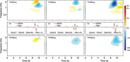
To further investigate the capacity of the collocated grid finite-difference scheme for seismic wave modelling in complex media, we perform a numerical simulation in a layer over a half-space model. The first layer is 1 km thick with a lower velocity (P wave velocity of 2 km s⁻¹ and S wave velocity of 1 km s⁻¹). Other parameters are shown in Table 2.

Table 2.

Model and simulation parameters for the flat layer over a half-space model.

Open in new tabDownload slide

The geometry of the source and receivers is illustrated in Fig. 5. The double couple source with strike = 0°, dip = 45° and rake = 90° is located 500 m below the free surface, in the middle of the first layer. In this numerical test, we employ a vertically variable grid size. The vertical grid sizes start at 50 m in the first layer and gradually increase to 125 m below the first layer to reduce memory requirements. For interior interfaces in the model, we use the effective media parameter approach of Moczo (2002). The model and simulation parameters can be found in Table 2.

Figure 5

Surface projection of the source-receiver geometry for the flat layer over a half-space model. The source (star) is located at (0, 0, −500) m, the middle of the first layer. There are total 11 receivers (triangle symbols) at the free surface, deployed every 1 km from x= 0 to x= 10 km along y= 10 km. The maximum source-receiver distance (at receiver 11) is about 15.4 times the dominant surface wave wavelength and about 38.4 times the minimum surface wave wavelength.

Open in new tabDownload slide

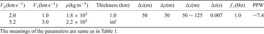
Figs. 6 and 7 show the TF misfit and goodness-of-fit at receivers 1 and 11, respectively. In comparison with the half space model, TFEM increases to below 20 per cent at receiver 11 due to complex reflections, while TFPM maintains a similar error level (around 5 per cent). We should note that the overall amplitude misfit for the entire seismogram at receiver 11 is satisfactory, which can be seen from the single-valued envelope misfit values for the three components. The 20 per cent maximum TFEM for the Uz component only occurs over a narrow time window.

Figure 6

Time-frequency envelope misfit (TFEM; top row) and phase misfit (TFPM, bottom row) between the FDM solutions (dash-dotted red line, middle row) and the reference GRTM solutions (solid black line, middle row) at receiver 1 for the layer over a half-space model with a flat surface. Left column: x component. Middle column: y component. Right column: z component. Values of the single-valued envelope goodness-of-fit (EG), phase goodness-of-fit (PG), envelope misfit (EM) and phase misfit (PM) are labelled in the middle row.

Open in new tabDownload slide

Figure 7

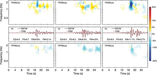
Time-frequency envelope misfit (TFEM; top row) and phase misfit (TFPM, bottom row) between the FDM solutions (dash-dotted red line, middle row) and the reference GRTM solutions (solid black line, middle row) at receiver 11 for the layer over a half-space model with a flat surface. Left column: x component. Middle column: y component. Right column: z component. Values of the single-valued envelope goodness-of-fit (EG), phase goodness-of-fit (PG), envelope misfit (EM) and phase misfit (PM) are labelled in the middle row.

Open in new tabDownload slide

5.3 Topographic model of a 3-D Gaussian-shaped hill

In this test, we compare the results of FDM and SEM determinations for a homogeneous medium with a geometrically defined topographic surface. This verifies the ability of the proposed collocated-grid FDM using traction image setting on a curvilinear grid to simulate seismic wave propagation in the presence of surface topography.

The surface topography is defined by a Gaussian function:

(44)

where a= 1000 m. The explosive source is located at x= 800 m, y= 0 and 100 m below the free surface. The locations of the source and receivers are shown in Fig. 8. This topographic model was designed by Ohminato & Chouet (1997) to test the implementation of the free-surface boundary conditions using a stair-case sgrid in the staggered-grid FDM. Janod & Coutant (2000) used this model to compare their time-domain boundary-element method with the SEM and the FDM of Ohminato & Chouet (1997). They found that the stair-case grid approximation could cause a greater phase distortion and artificial scattering. In this test, we use this model with the same source and receiver settings to verify our FDM scheme by comparisons with SEM.

Figure 8

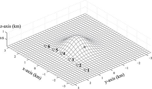
Source and receiver locations for the topographic model with a 3-D Gaussian-shaped hill. The hill is of the shape z(x, y) = 1000 exp (− (x²+y²)/1000²) with the maximum height of 1000 m. The topography is shown as the surface computation grid points with a decimation factor of 4. The source is located inside the topographic region with x=−800 m, y= 0 m and vertically 100 m below the free surface. The epicentre location is shown as a star in the figure. There are six receivers, deployed every 800 m along the x-axis at the surface along y= 1300 m. The horizontal coordinates of the six receivers are (− 2400, 1300), (− 1600, 1300), (− 800, 1300), (0, 1300), (800, 1300) and (1600, 1300).

Open in new tabDownload slide

Table 3 shows the model and simulation parameters for this numerical test. The source is located near the surface (100 m depth, note that the dominant Rayleigh wavelength is around 920 m) and can generate strong energy in high-frequency Rayleigh waves. To increase the resolution for the Rayleigh waves, we use a finer vertical grid size (half the horizontal grid size) near the surface, as shown in Fig. 9.

Table 3.

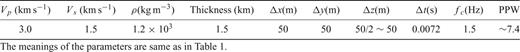
Model and simulation parameters for the Gaussian hill model.

Open in new tabDownload slide

Figure 9

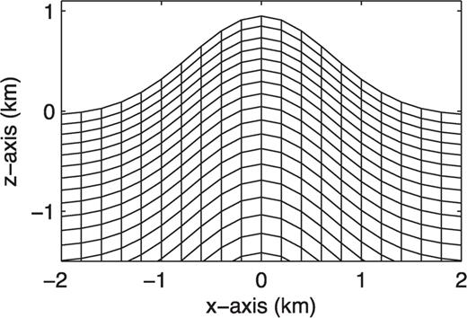
Vertical grid structure near the peak of the Gaussian hill shown on the x−z slice. Only one of every four points in the horizontal and vertical grid are shown. The horizontal grid size is 50 m. The vertical grid size is around 25 m near the surface and gradually increases to 50 m at depth.

Open in new tabDownload slide

Fig. 10 shows the displacement from our FDM against the solution from SEM. The overall fit is very good. Fig. 11 shows the time-frequency envelope and phase misfit at receiver 3, which is nearest to the source, while Fig. 12 is for receiver 6, which is farthest from the source. In general, the agreement of the phase misfit is better than the envelope misfit.

Figure 10

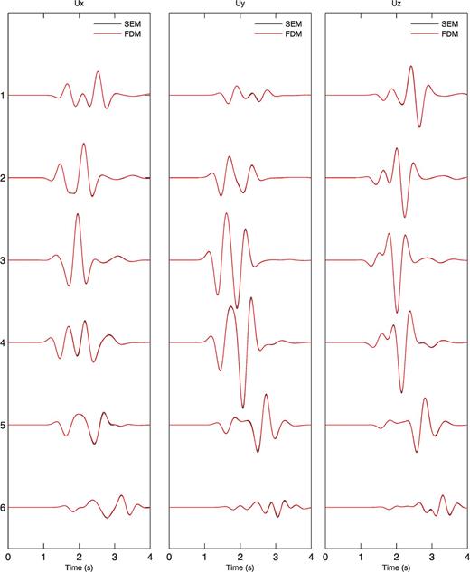
Comparison of the three displacement components between FDM and SEM at surface receivers 1 to 6 for the Gaussian hill model. Left: x component. Middle: y component. Right: z component. Black lines are SEM results and red lines are FDM results.

Open in new tabDownload slide

Figure 11

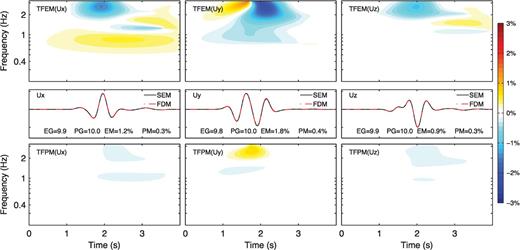
Time-frequency envelope misfit (TFEM; top row) and phase misfit (TFPM, bottom row) between the FDM solutions (dash-dotted red line, middle row) and the reference SEM solutions (solid black line, middle row) at receiver 3 (the third trace in Fig. 10) for the Gaussian hill model. Left column: x component. Middle column: y component. Right column: z component. Values of the single-valued envelope goodness-of-fit (EG), phase goodness-of-fit (PG), envelope misfit (EM) and phase misfit (PM) are labelled in the middle row.

Open in new tabDownload slide

Figure 12

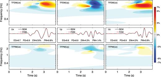
Time-frequency envelope misfit (TFEM; top row) and phase misfit (TFPM, bottom row) between the FDM solutions (dash-dotted red line, middle row) and the reference SEM solutions (solid black line, middle row) at receiver 6 (the 6th trace in Fig. 10) for the Gaussian hill model. Left column: x component. Middle column: y component. Right column: z component. Values of the single-valued envelope goodness-of-fit (EG), phase goodness-of-fit (PG), envelope misfit (EM) and phase misfit (PM) are labelled in the middle row.

Open in new tabDownload slide

This numerical test verifies that using the collocated-grid FDM, with the traction image setting, and curvilinear grids can simulate seismic wave propagation in the presence of surface topography with sufficient accuracy.

6 Conclusions

In this paper, we use curvilinear grids and the higher order collocated finite-difference scheme, DRP/opt MacCormack, to solve the first-order hyperbolic velocity-stress equations in the presence of surface topography.

In the DRP/opt MacCormack scheme, all the velocity-stress components are defined at the same spatial position in a grid cell. Such a grid is called a non-staggered or collocated grid. To overcome the odd-even decoupling oscillation associated with the central difference operator on the collocated grid, the DRP/opt MacCormack scheme alternately uses forward and backward difference operators in the Runge-Kutta time stepping method. It has fourth-order accuracy for the dispersion error, and is optimized for the dissipation error for eight or more points per wavelength.

To eliminate the artificial scattering caused by a stair-case grid approximation of the topography, we use a curvilinear grid (also known as a boundary-conforming or body-fitted grid) to conform the grid plane with the surface topography. This boundary-conforming grid is represented by general curvilinear coordinates, in which the velocity-stress equations contain more differential terms than in the Cartesian coordinate because of the coordinate transform. The implementation of the DRP/opt MacCormack scheme for these general curvilinear coordinates is the same as for the Cartesian coordinates, because all of the variables are located at the same grid point in the DRP/opt MacCormack scheme.

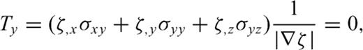
The boundary-conforming grid transforms the irregular surface in the physical space into a ‘flat’surface in the computational space. The free-surface boundary conditions are implemented at this ‘flat’surface. When topography is present, none of the single stress components is zero at the free surface. Therefore, we propose the use of a traction image technique, which antisymmetrically images the traction components with respect to the free surface. To use this technique, we rewrite the momentum equation in a conservative form, in which the differentiated quantities are the traction components.

Note that the proposed traction image method is not restricted to the DRP/opt MacCormack scheme used in this paper. We chose the DRP/opt MacCormack scheme because of its simple and easy implementation. The traction image method also can be used in other collocated grid finite-difference schemes, for example compact schemes and schemes involving optimal centre differences with explicit filtering.

We performed three numerical tests to verify the use of: (i) curvilinear grids, (ii) the collocated finite-difference scheme and (iii) the traction image technique to simulate seismic wave propagation. The simulations were compared with those from the generalized reflection/transmission coefficients method and spectral-element method. The comparisons verify that using the curvilinear grid, collocated finite-difference scheme and traction image technique we can simulate seismic wave propagation in presence of the surface topography with sufficient accuracy.

7 Acknowledgments

The SPECFEM3D package from CIG () was used to generate the SEM solution for the Gaussian hill model. We appreciate Hejun Zhu's help on the SEM simulations. We are grateful to Peter Moczo and another anonymous reviewer for their constructive comments. This research was supported by National Science Foundation of China (grant numbers 41090293, 40874019).

Appendices

Appendix A: Coordinate Metric

Once the free surface topography is given, algebraic or PDE (partial differential equation) methods can be used to generate the boundary-conforming grid. The grid qualities, estimated in terms of the concentration of grid points, smoothness of the variations in grid size and orthogonality of the grid, can be controlled during generation (Thompson 1985). Numerical grid generation as a basic step in many scientific computing problems has been developed over a long period of time and has become a fairly common tool in the numerical solution of partial differential equations (Thompson 1985).

After the boundary-conforming grid is generated, the Cartesian coordinates of each discrete grid point can be determined. Thus the mapping from curvilinear to Cartesian coordinates is,

(A1)

and their derivatives can be numerically calculated using the same numerical scheme for the elastic wave equations,

(A2)

where D_ξ, D_η and D_ζ represent the difference operators of the spatial derivatives ∂_ξ, ∂_η and ∂_ζ. Note that even when the mapping equation (A1) is given by an analytical function, the coordinate transform derivatives still should be calculated numerically to avoid spurious source terms when conservation forms of the momentum equations are used (Thompson 1985).

From the relationships:

(A3)

we can get the coordinate metrics needed in eqs (23)#x2013;(26),

(A4)

In these equations, J is the Jacobian of the transformation, which is ensured to be non-zero during the grid generation process (Thompson 1985),

(A5)

Appendix B: Unit Vector Perpendicular to the Free Surface

A general curvilinear coordinate has two sets of base vectors, covariant base vectors:

(B1)

(B2)

(B3)

and contravariant base vectors:

(B4)

(B5)

(B6)

The relationship between these two sets of base vectors is

(B7)

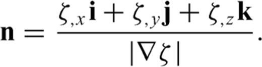
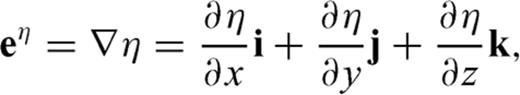
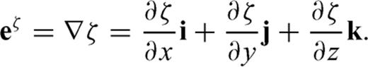
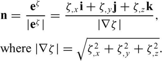
The covariant base vectors are parallel to the coordinate plane; for example in our applications, and are parallel to the topography at the free surface. From eq. (B7), we can see is normal to the free surface, thus the unit vector perpendicular to the free surface is

(B8)

where .

Appendix C: Conservative Form of the Momentum Conservation Equations

In curvilinear coordinates, operator has two forms (Thompson 1985)

Conservative form:

(C1)

Non-conservative form:

(C2)

where ξⁱ∈{ξ, η ζ}, J is the Jacobian of the transformation and are the contravariant base vectors (eqs B4–B6).

Substituting the conservative form of the operator ▽ into the momentum conservation equation 1, we can derive the conservative form of the momentum equation in curvilinear coordinates as

(C3)

(C4)

(C5)

Substituting eqs (29)–(31) into the above equations, we can derive eqs (39)–(41) that can utilize the antisymmetric property of the traction.

References

Author notes