Comparison of decay features of the 2006 and 2007 Kuril Island earthquake tsunamis

Summary

1 Introduction

The appearance of time-series tsunami waveforms differ depending on the tsunami event and the tidal station at which they are recorded. The reason for this variability has been only partially determined. Watanabe (1998) categorized tsunami waveforms into three types based on their shape. Some characteristics of the later phases of tsunamis have been discussed, such as edge waves (González 1995) and scattered waves (Mofjeld 2001). Saito & Furumura (2009) formulated a theory of tsunami coda excitation and attenuation of leading waves due to scattering by ocean—floor topography. The characteristics of the later phases are an important factor when deciding whether to cancel a tsunami warning. However, numerical tsunami modelling remains inadequate in providing accurate waveforms, even many hours after the arrival of the initial wave. This is probably because of the complexity of the tsunami source, the path and site effects and numerical calculation errors, such as those due to diffusion.

Lack of technology for forecasting tsunami decay or the later phase of tsunamis can cause serious failures in tsunami warning systems. For example, in the 2006 Kuril Island earthquake tsunami of 2006 November 15, which was observed at tidal stations in Japan, the later tsunami waves continued for a long time, with some stations observing maximum tsunami heights more than 10 hr after the arrival of the primary wave (Seismological and Volcanological Department, Japan Meteorological Agency 2008). However, by that time, the tsunami warning to these areas had already been cancelled by the Japan Meteorological Agency (JMA).

If the overall tsunami waveform pattern could be determined in advance or in real time, it would enable us to forecast the tsunami decay. Hayashi (2009) demonstrated that the tsunami coda may become a useful measure for characterizing the tsunami decay process through the analysis of observed tsunami waveforms generated by the 2006 Kuril Island earthquake. In this paper, we describe the definition of three terms: the ‘moving root mean squared amplitude’ (MRMS amplitude), ‘tsunami coda’ and ‘non-dimensional tsunami amplitude’ (NDA). We then compare the characteristics of the decay features of the 2006 and 2007 Kuril Island earthquake tsunamis by applying these measures.

2 Definitions of Terms

To facilitate the discussion of the tsunami decay process, we define ‘MRMS amplitude’, ‘tsunami coda’ and ‘NDA’ as depicted in Fig. 1.

Figure 1

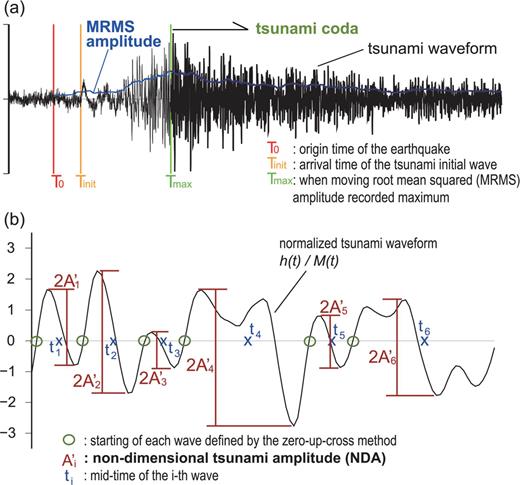
Definitions of (a) moving root mean squared (MRMS) amplitude and tsunami coda and (b) non-dimensional amplitude (NDA).

Open in new tabDownload slide

2.1 MRMS amplitude

The MRMS of a time-series sea level anomaly is calculated as

1

where t is time, M(t) is the MRMS amplitude at t, w is the width of the moving window and h(t) is the sea level above the datum at t. M²(t) should represent the time-series of half of the tsunami energy observed at a certain site if the noise level is negligible. Furthermore, for time-homogeneous sine waves, √2 M(t) should be equivalent to a single amplitude of a wave. The value of w should be larger than the typical wave period so that the MRMS amplitude relates to the time-series of typical single amplitude.

The corrected MRMS amplitude can be calculated with the background level taken into account by

2

where M′(t) is the corrected MRMS amplitude at t and M_BGL is the background level rms of the sea level anomaly during normal times (with no tsunamis).

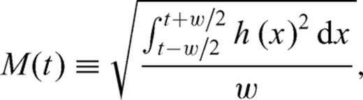
By applying this definition of corrected MRMS amplitude to a tsunami waveform, the trend of the typical single amplitude, which is approximately proportional to the tsunami energy flux at a specific station, can be extracted from the complexity of the waveform.

2.2 Tsunami coda

To discuss the decay processes of tsunami waveforms, we define the tsunami coda as the part of the tsunami waveform after T_max, the time of the recorded maximum MRMS amplitude. This definition is different from that of the seismic coda. The seismic coda wave was originally regarded as the later part of the waveform, which was considered to consist of scattered waves originating from outside the seismic source (Aki 1969). More recently, the seismic coda has come to be regarded as the part just after the wave train of a specific phase, for example, the P phase or S phase (Sato & Fehler 1997). Saito & Furumura (2009) implicitly defined the tsunami coda as the part of a waveform that appears to be controlled by scattering behaviour caused by fluctuations of the ocean—floor topography. However, such scattering may be one of various phenomena affecting the tsunami decay process and this implicit definition of tsunami coda is inconvenient when discussing a tsunami decay process mainly controlled by factors other than scattering.

Here, we separate the tsunami waveform into two parts: the coda, which is part of the decay process and the preceding part, in which the amplitude of the tsunami increases (Fig. 1a). This definition enables us to analyse the tsunami decay process without emphasizing particular factors.

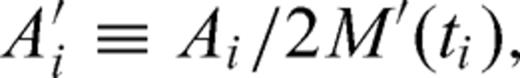
2.3-NDA

We define NDA as

3

where i is the order of the wave extracted from the tsunami coda using the zero-crossing method, A_i is the crest-to-trough amplitude of the ith wave, A′-_i is the NDA of the ith wave and t_i is the midtime of the ith wave. A set of NDAs in the tsunami coda for each station was calculated by using the zero-crossing method (Fig. 1b).

3 Application to the 2006 and 2007 Kuril Island Earthquake Tsunamis

3.1-2006 and 2007 Kuril Island earthquakes

The 2006 Kuril Island earthquake (A in Fig. 2) occurred along the Kuril trench at 20:14 on 2006 November 15 (Japan Standard Time (JST); JST = UTC + 9 hr). Its mechanism was considered to be a reverse fault type and its moment magnitude (M_w) determined by the Global Centroid Moment Tensor Project (Global CMT Project; ) was 8.3. The 2007 Kuril Island earthquake (B in Fig. 2) occurred in the Pacific Plate at 13:23 on 2007 January 13. Its mechanism was normal faulting and its magnitude was determined as M_w 8.1 by the Global CMT Project.

Figure 2

Locations of tidal stations (circles) whose data are used in this study. Tidal stations indicated by red circles are referenced in Figs 4, 6 and 7.

Open in new tabDownload slide

Both earthquakes generated tsunamis that affected the coasts of the Okhotsk Sea and Pacific Ocean and the Izu—Bonin—Mariana Island arc (IBM arc) of Japan. Both tsunamis were accompanied by significant later phases; maximum amplitudes were recorded in later phases at most stations and waves continued for a long time before decaying completely (Seismology and Volcanology Division, JMA 2008).

3.2 Tsunami waveform data

We used sea level time series data sampled every 15 s from tidal stations (Fig. 2) operated by JMA. For greater accuracy of the analysis, data were selected from tidal stations at which a maximum amplitude of over 0.25 m was recorded. To eliminate the effects of the astronomical tide, we used smoothed hourly sea level data provided by JMA. Furthermore, the effects of short period non tsunami sea waves, such as wind waves, were filtered out using a low pass finite impulse response (FIR) digital filter with a 2 min cut off period.

We used data from the 2006 Kuril Island earthquake tsunami from 32 tidal stations that satisfied the above criteria. One of them (Abashiri) faces the Okhotsk Sea, another (Makurazaki) faces the East China Sea and the rest are located along the Pacific coast. We used data from 14 stations for the 2007 Kuril Island earthquake tsunami, all located along the Pacific coast.

3.3 Time series of MRMS amplitude and tsunami coda

Tsunami traveltimes (T_dir) from the source of the 2006 and 2007 Kuril Island earthquakes to each tidal station were calculated by Huygens' principle using the ‘Tsunami Travel Time program’ (Geoware) and 2 min grid bathymetry data generated from ETOPO1 (Amante & Eakins 2009). Tsunami traveltimes (T_scat) from the seismic source to each station via Kinmei Seamount, the southernmost of the Emperor Seamounts, were also calculated as the sum of the first tsunami arrival time at Kinmei Seamount and the traveltime from the seamount to each station (Fig. 3).

Figure 3

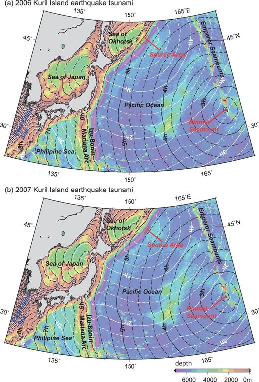
Isograms of traveltimes of the 2006 and 2007 Kuril Island earthquake tsunamis. White lines are isograms of calculated traveltimes of the tsunami fronts. Tsunami source areas indicated by thin red lines, assumed to be just above the subfaults derived by inversion of tsunami waveforms (Fujii & Satake 2008). Black lines indicate traveltimes of scattered tsunami waves generated by reflection from Kinmei Seamount.

Open in new tabDownload slide

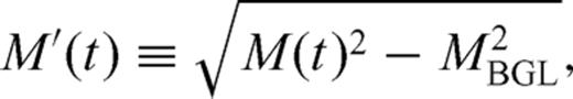
Using the definition in Section 2.1, the time series of the MRMS amplitude at each station was calculated using a 64 min moving window and background level for each station measured from data observed during the 3 hr period just before the earthquake. The tsunami coda, as defined in Section 2.2, was the part of the tsunami waveform after the maximum MRMS amplitude. Examples of time series of MRMS amplitudes and tsunami codas from eight tidal stations are plotted in Fig. 4.

Figure 4

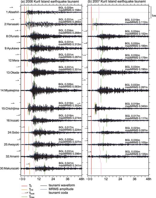
Examples of waveforms and tsunami codas of the 2006 and 2007 Kuril Island earthquake tsunamis observed at tidal stations. x axes indicate hours from the earthquake occurrence. Station locations are in Fig. 2. BGL indicates a background level determined from observation data during the 3 hr period just before the earthquake.

Open in new tabDownload slide

Koshimura (2008) showed that the waveforms of the 2006 Kuril Island earthquake tsunami observed in Japan had remarkable later phases due to scattering by the Kinmei Seamount. The orders of T_max and T_scat plotted in Fig. 4 indicate that the tsunami codas recorded at Abashiri, which faces the Okhotsk Sea and Chichijima, which is located on the IBM arc, began before the estimated arrival time of the scattered wave. They also show that at the other stations along the Pacific Ocean or the East China Sea, the tsunami coda began after the estimated arrival time of the scattered wave. Based on computed visualizations of tsunamis, Koshimura (2007) pointed out that the paths of the 2006 tsunami to Japan consisted of (1) the direct wave from the source, (2) multiple reflections from the shelf along the Pacific Ocean and (3) waves scattered by the Emperor Seamounts. The codas of the 2006 tsunami employed in this study can be characterized as (2) or (3). In addition, the choice between (2) and (3) at each site can be roughly assessed by whether T_max precedes T_scat or follows it.

3.4 Decay time function of corrected MRMS amplitude

The time series of the MRMS amplitudes at each station up to 48 hr after the earthquakes (Fig. 5) shows that the decay of the MRMS amplitudes is approximately exponential. Regression analysis of the corrected MRMS amplitude was performed to fit the formula

4

where t is the time since the earthquake occurred; M′-(t) is the corrected MRMS amplitude at t, defined by eq. (2); τ is the decay time constant to be solved and k is a proportionality constant. The parameter τ in eq. (4) represents the time necessary for the corrected MRMS to fall to 1/e of its initial value. In other words, τ is the period of half decay multiplied by 1.44. Tsunami codas from T_max+w/2 to T_o+ 48 hr were used for the regression analysis. However, for accuracy, data were not used from periods when the signal to noise ratio estimated from the background level obtained in Section 2.1 was less than 1.0. For this reason, four stations were rejected for the 2006 tsunami and three stations were rejected for the 2007 tsunami.

Figure 5

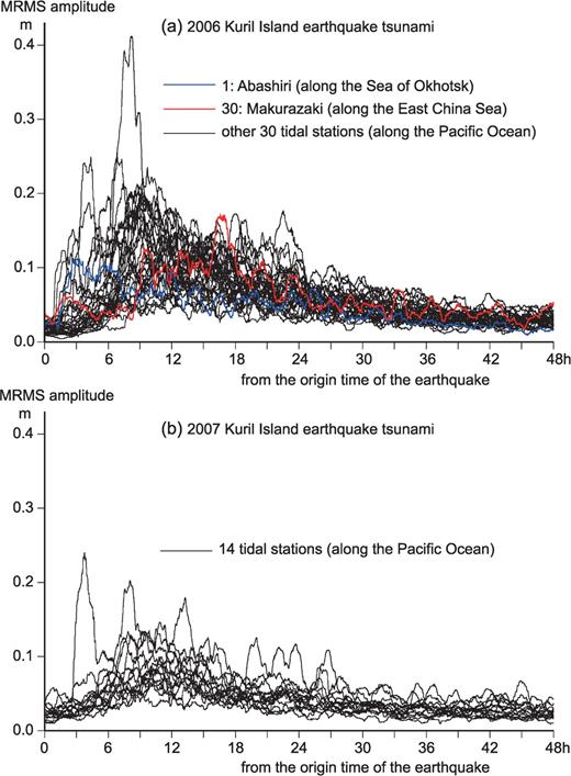
Time series of MRMS amplitudes of (a) the 2006 and (b) the 2007 Kuril Island earthquake tsunamis observed at tidal stations listed in Table 1. x axis indicates hours from the earthquake occurrence.

Open in new tabDownload slide

For the 2006 tsunami, decay time constants for the time series of the corrected MRMS amplitudes were obtained from 28 of the 32 stations (Table 1a). The decay time constants from the 26 Pacific stations ranged from 12.8 to 26.5 hr. The average value and its standard deviation (SD) for these 26 stations were 20.1 and 3.3 hr, respectively. The differences between this average value and all the decay time constants derived from the individual tidal stations along the Pacific coast except for Hachinohe, Toba and Uragami were within only 25 per cent. This average value of the decay time constant for the Pacific Ocean stations (20.1 hr) differed significantly from that at the Abashiri station (28.0 hr) along the Okhotsk Sea and at the Makurazaki station (13.1 hr), which faces the East China Sea; these results are in agreement with those of Hayashi (2009). The 26 Pacific stations were classified into three groups: stations northeast of the IBM arc, stations on the IBM arc and stations west of the IBM arc (in the Philippine Sea). The averaged decay time constants for these groups had no significant differences among them (Table 1a). These results suggest that the decay time constant measured by corrected MRMS amplitude in the coda of the 2006 tsunami depends mostly on which ocean the station is facing.

Table 1

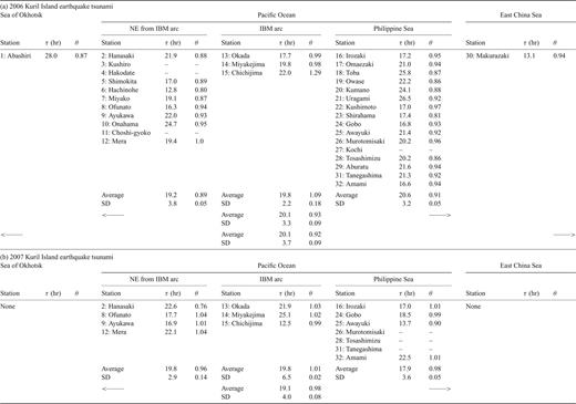
Constants related to time decay and fluctuation of amplitudes in tsunami codas of the 2006 and 2007 Kuril Island earthquake tsunamis. Decay time constants (τ; eq. 4) of corrected MRMS amplitude and the maximum likelihood estimators (θ; eq. 5) of the Rayleigh distribution model for appearance frequency of NDAs in tsunami codas are listed. Station locations are in Fig. 2. Dashes indicate stations where the signal-to-noise ratio of the data is below 1.0.

Open in new tabDownload slide

For the 2007 tsunami, decay time constants of the time-series of corrected MRMS amplitudes were obtained from 11 of the 14 stations, all of them facing the Pacific (Table 1b). The decay time constants ranged from 12.5 to 25.1 hr, averaging 19.1 hr with an SD of 4.0 hr. The 11 stations were classified in the same manner as the 2006 tsunami stations facing the Pacific and again, no significant differences were found (Table 1b). The differences between the average decay time constants (eq. 4) for the Pacific coast of Japan (τ= 20.1 hr for the 2006 tsunami and 19.1 hr for the 2007 tsunami) and most of the decay constants derived from the individual tidal stations along the Pacific coast are within only 25 per cent (Table 1).

3.5 Appearance frequencies of NDA in tsunami coda

The appearance frequencies of the NDAs in each tsunami coda at 13 typical stations are shown for the 2006 tsunami in Fig. 6 and similar results are shown for all 11 stations for the 2007 tsunami in Fig. 7. These figures also show merged results for both sets of stations, which are listed in Table 2.

Figure 6

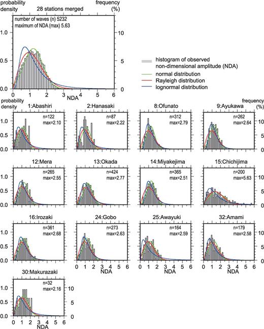
Distribution of appearance frequency of NDAs in tsunami codas of the 2006 Kuril Island earthquake tsunami and comparison of stochastic models. Histograms of appearance frequency of NDAs in tsunami coda include probability density functions (Rayleigh distribution, normal distribution and lognormal distribution) with maximum likelihood model parameters. Station locations are in Fig. 2.

Open in new tabDownload slide

Figure 7

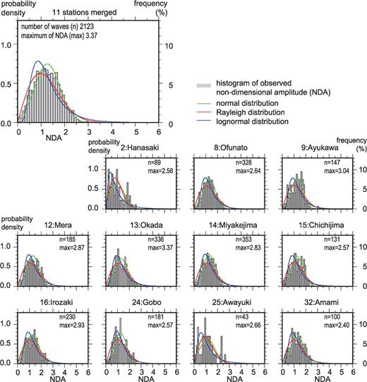
Distribution of appearance frequency of NDAs in tsunami codas of the 2007 Kuril Island earthquake tsunami and comparison of stochastic models.

Open in new tabDownload slide

Table 2

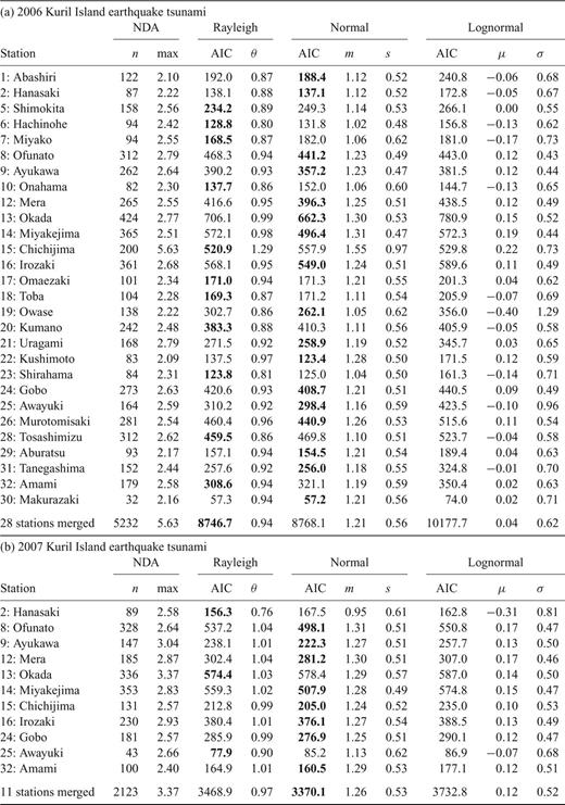
Comparison of AICs of three stochastic models and their maximum likelihood estimators of the 2006 and 2007 Kuril Island earthquake tsunamis. Figures in boldface indicate minimums of AICs. Model parameters are defined in eqs (5)–(7). Station locations are in Fig. 2.

Open in new tabDownload slide

Comparisons using the Akaike Information Criterion (AIC; Akaike 1974), shown in Figs 6 and 7, indicate that the Rayleigh distribution, defined by

5

or the normal distribution, defined by

6

approximate these appearance frequencies of NDA better than the log-normal distribution, defined by

7

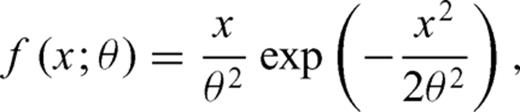
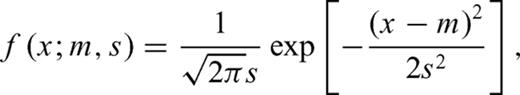
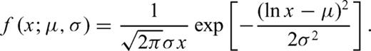
Here, f is the probability density function, x is the NDA and θ, m, s, μ and σ are the model parameters for each probability density function.

For the 2006 tsunami, the AIC comparison shows that the Rayleigh distribution best explains the appearance frequency of the merged NDAs, with the normal distribution ranking second. However, when applied to each station separately, the Rayleigh distribution is the best model for some stations and the normal distribution is best for others (Table 2a). Practically, the Rayleigh distribution is easier to apply because it has only one model parameter, whereas the normal distribution has two. As listed in Table 2(a), the Rayleigh distribution parameters determined by the maximum likelihood method ranged between 0.80 and 0.99 for all stations except for the Chichijima station, located on the IBM arc. This suggests that the distribution of NDA is almost station-independent and ocean-independent.

For the 2007 tsunami, the AIC comparison shows that the normal distribution best explains the appearance frequency of the merged NDAs, with the Rayleigh distribution ranking second. However, the Rayleigh distribution was the best model for some individual stations (Table 2b). As listed in Table 2(b), the Rayleigh distribution parameters determined by the maximum likelihood method ranged between 0.76 and 1.04. The average of the model parameters is 0.97, which is very close to the average for the 2006 tsunami (0.94).

4 Discussion and Summary

We defined and discussed the terms ‘MRMS amplitude’‘tsunami coda’ and ‘NDA’ (Section 2 and Fig. 1) and then applied them to the analysis of time-series sea level data of 2006 and 2007 Kuril Island earthquake tsunamis with different seismic mechanisms (Section 3).

Our analysis reveals that MRMS amplitudes in tsunami codas corrected for background level decay exponentially with time. This demonstrates that the station dependency of decay time constants along the Pacific Coast was small for these two tsunamis. However, the decay time constants for the 2006 tsunami at the stations along the Okhotsk Sea and the East China Sea differ significantly from the Pacific average values (Section 3.4 and Fig. 5).

Our results also indicate that the wave height fluctuation can be approximated by either the normal distribution or the Rayleigh distribution (Figs 6 and 7; eqs 5 and 6). The latter is well known as the probability density function for appearance frequency of amplitudes of incoherent composite waves, such as wind swells. In addition, the maximum likelihood parameter of the Rayleigh distribution was similar for all tidal stations except for Chichijima station, located on the IBM arc (Section 3.5; Figs 6 and 7). From the analogy of wind swells, these stochastic characteristics of wave amplitudes appearing in tsunami codas suggest that the tsunami decay process of the 2006 and 2007 tsunamis was characterized more by large-scale tsunami propagation in the form of incoherent waves, incorporating multiple reflections from continental shelves or trans-ocean multipath propagation rather than by a combination of a wave progressing towards a coast and waves trapped in a port or a bay.

The tsunami coda, as introduced by Hayashi (2009) or Saito & Furumura (2009) and updated in this study, can lead to a new understanding of the tsunami decay process. The application of MRMS amplitude and tsunami codas to the issue of improving tsunami warnings highlights two related problems: how to model the time-series decay of MRMS amplitudes and how to formulate stochastic behaviour in the tsunami decay process. Additional case studies may raise the potential of utilizing these measures for tsunami forecasting issues such as the timing of tsunami warning cancellations.

Acknowledgments

Thanks are due to two anonymous reviewers for their valuable comments and helpful suggestions. This paper is based on a part of the doctoral thesis by the first author (Hayashi 2010) with supervision by the other two authors. This research was supported in part by grants from the Maeda Engineering Foundation (No. Civil Eng.-1, 2009 year) and the Kajima Foundation (2009 and 2010 years). Tidal observation data were provided by the Global Environment and Marine Department, JMA. Some of the figures were prepared using Generic Mapping Tools (Wessel & Smith 1998). The authors gratefully acknowledge the helpful discussions with Dr. M. Hoshiba (Meteorological Research Institute) on interpreting characteristics of tsunami coda and the assistance of Ms. F. Hayashi in designing the figures.

References