Evaluation of intrinsic velocity—pressure trends from low-pressure P-wave velocity measurements in rocks containing microcracks

Summary

1 Introduction

Numerous laboratory experiments have shown that the elastic behaviour of rocks as a reaction on confining pressure P is mainly controlled in two ways: (i) the reduction of porosity and the progressive closure of microcracks, termed ‘extrinsic’ effects (ii) the ‘intrinsic’ effects on the crystal lattice of the rock constituents (e.g. Birch 1960). In experiments, the velocity–pressure trend is characterized by rapid non-linear increase of the elastic (P-, S-) wave velocities at low pressure mainly as a consequence of the ‘extrinsic’ effects, and a much smaller approximately linear increase of the elastic wave velocities at higher pressure due to the ‘intrinsic’ effects (Fig. 1). The shape of the velocity–pressure equation depends on several parameters such as the rock composition, porosity and the direction in which the velocity is measured (anisotropy; e.g. Siegesmund 1996). Thus, the transition from non-linear to linear velocity change (the ‘crack closure pressure’) is largely sample-dependent.

Figure 1

Relationship between wave velocitiy V and confining pressure P (schematic). V₀: zero pressure velocity in the experiment; Vⁱ₀: ‘intrinsic’ zero pressure velocity; dV/dP: ‘intrinsic’ pressure derivative; P_c: ‘crack closure pressure’, at which the ‘extrinsic’ effects vanish. The maximum pressure in the experiment is usually lower than P_c.

Open in new tabDownload slide

For mantle rocks, Christensen (1974) reports crack influence up to 1000 MPa, that is, experiments to pressures much larger than 1000 MPa are required to prove constant velocity gradients. However, actual equipment is often restricted to lower pressures, for example, 400 MPa (Pros et al. 1998) or 600 MPa (Kern et al. 2002). Frequently, it may be desirable to extrapolate velocity trends to pressures beyond the measuring range, especially for investigating composition of the lower continental crust, which requires velocity data at pressures of 500 MPa to as high as 1500 MPa. Such extrapolation applying model functions is possible (Ullemeyer & Popp 2004), but the accuracy of the extrapolated velocities—especially at very high pressures—has not been verified.

Furthermore, prediction of the ‘intrinsic’ velocity trend from the experimental velocity data may be desirable for describing the crack influence at low pressures in a quantitative way. Due to lattice preferred orientation and elastic anisotropy of the rock constituents (e.g. Mainprice et al. 2000), which control the ‘intrinsic’ velocity trend, and due to anisotropy of the crack fabric (e.g. Siegesmund et al. 1993), both the experimental and the ‘intrinsic’ velocity trend vary in dependence on the sample direction considered in the experiment. If, for example, the whole set of elastic constants needs to be calculated from 3-D spherical sample measurements, such anisotropic property of the sample is significant, because the results of the calculations are highly sensitive to imposed starting values (Klima 1973; Jech 1991). Especially the comparison of ‘bulk rock’ and ‘intrinsic’ elastic constants—synonymous to the above-mentioned quantitative description of the crack fabric—requires accurate experimental data and reliable estimates of the ‘intrinsic’ velocity trend as well.

In field seismics, laboratory estimates of the elastic wave velocities are useful for the processing of geophysical data, the explanation of seismic structures and the verification of P- and S- wave velocity versus depth relationships in the Earth's crust (Christensen & Mooney 1995; Lin et al. 2010). Empirical relations between particular wave velocities, density (ρ) and Poisson's ratio (σ) are used to infer, for example, S-wave velocity, ρ or σ from P-wave measurements (Brocher 2005 and references therein). To ensure comparability of field and experimental data, the error of the laboratory measurements should be much better than the effect to be described. To give an example, a 10 per cent serpentinization of ultramafic rocks decreases P-wave velocity by about 0.3 km s⁻¹ (Christensen 1966, 1978), consequently, the overall error of an experiment to verify such effect should significantly fall below this magnitude.

The pressure dependence of the elastic wave velocities and the ‘intrinsic’ velocity trend in a distinct sample direction may be derived from mechanical theories (e.g. Levin et al. 2004 and references therein). However, the modelling requires information on fabric parameters like rock composition, elastic constants and crystallographic preferred orientations of the rock constituents, crack density, crack aspect ratio and crack orientation. In this study, we want to propose a solely empirical solution for the extrapolation of velocity–pressure trends from low-pressure velocity measurements, emphasizing in particular determination of the ‘intrinsic’ velocity–pressure trend, which is given by the velocity at zero pressure, Vⁱ₀, and the ‘intrinsic’ pressure derivative, dV/dP (Fig. 1). Focusing on determination of the ‘intrinsic’ velocity trend is motivated by its significance for the quantification of the crack influence on the elastic wave velocities, as denoted above. Moreover, the ‘intrinsic’ velocity trend fully describes the velocity trend at high pressure. Except for experimental data the method requires no additional input and is, therefore, applicable even in case of completely missing fabric information about the sample under investigation.

First, we checked several model functions proposed in the literature with respect to their suitability for extrapolation. P-wave measurements on four samples (amphibolite, pyroxenite, serpentinite and metagabbro) with different crack closure behaviour and velocity magnitudes were performed at Department of Geology and Geophysics, Madison, University of Wisconsin, USA within the pressure range 10 MPa ≤P≤ 1000 MPa. The pressure range from 10 MPa to 600 MPa was used to fit model functions to the data and the P-wave trends given by the model functions were extrapolated to 1000 MPa. The P-wave data measured at 800 and 1000 MPa served as a reference to verify reliability of the extrapolated data. Secondly, P-wave measurements on two more samples (amphibolite and gneiss) at Institut für Geowissenschaften, Kiel, Germany are used to demonstrate how the ‘intrinsic’ pressure gradient may be determined more accurately from lower pressure experiments to P_max = 600 MPa. For description of the laboratory equipment refer to Christensen (1985) and Kern et al. (2002), respectively. Accuracy of the velocity measurements at Madison is reported to be ≪1 per cent (Christensen 1985), however, due to missing correction for sample compression, the bulk error increases to about 1 per cent (Birch 1960). The overall error of the Kiel data was determined to be <1 per cent (Kern et al. 2002). In view of the goals of this study, such error level is of minor significance.

2 Suggested Model Functions from the Literature

Several relations were proposed to describe the pressure dependence of the elastic wave velocities in rocks; Greenfield & Graham (1996) provide earlier references. Wepfer & Christensen (1991) used a superposition of two exponential functions,

1

which appears to describe velocity—pressure trends of many rocks well (the subscript 1 denotes eq. (1), etc., throughout the manuscript). For 0 < b₁ < 1 and 0 < d₁ < 1, respectively, both terms of eq. (1) are characterized by monotonous growth for P→∞; the approximated gradient is assumed to resemble the ‘intrinsic’ pressure derivative dV/dP. However, the constants a₁, b₁, c₁ and d₁ are solely empirical and give no direct description of the ‘intrinsic’ velocity trend. The relation proposed by Pros et al. (1998),

2

is based on the assumption that the ‘intrinsic’ velocity increase with increasing confining pressure is linear and the ‘extrinsic’—first of all crack-induced—velocity increase with increasing pressure may be described by an exponential term. The constants a₂, b₂, c₂ and d₂ are related to the physical state of rock such that a₂ is the velocity at zero pressure, b₂ is the assumed ‘intrinsic’ pressure derivative of the crack-free sample, c₂ is the crack influence on velocity at atmospheric pressure, d₂ is the confining pressure at which the non-linear crack influence is reduced to 10 per cent. The relation proposed independently by Freund (1992) and Greenfield & Graham (1996) uses base ‘e’ instead of base 10 in the exponential term of eq. (2), that is, both relations are similar with the exception that the ‘crack closure parameter’d₂ does not bear any direct physical relationship to the crack closure behaviour. Since the elastic constants are directly proportional to the square of the elastic wave velocities, Greenfield & Graham (1996) also discussed suitability of the squared form of eq. (2), but concluded that most experimental velocity–pressure trends may be adequately described by the linear relationship. Wang et al. (2005) tried to detect the critical pressure, P_c, where the transition from non-linear to linear velocity change takes place. They modelled the entire velocity–pressure trend as being described independently by two relations,

3a

3b

where eq. (3a) is used to fit the data in the non-linear regime and eq. (3b) models the ‘intrinsic’ velocity trend with pressure. The procedure works as follows: first, the experimental data are replaced by a smoothing spline function of 1 MPa interval step size. Secondly, P_c is determined on the basis of the correlation coefficient r² for the linear fit in the pressure range P_c≤P≤P_max (P_max is the maximum pressure used in the experiment), which should exceed a given threshold. Starting at the lowest pressure and assuming it is P_c, eq. (3b) is to be fitted to the data. Whenever r² < threshold, the next value of the spline function is taken as P_c until r²≥ threshold. Although the method is applicable for P_c < P_max only, it is superior to the often-used intuitive definition of P_c and, therefore, considered in the following.

3 Results of Fit and Extrapolation

Eqs (1), (2) and (3a)/(3b) were fit to the increasing pressure loop of the experimental data obtained at Madison in the pressure range 10 MPa ≤P≤ 600 MPa. Visual judgement of the fits (Figs 2(a)–(c)) as well as RMS errors (Table 1) confirm close agreement of the model functions to the experimental data. Frequently, the RMS errors are at least one order of size less than experimental errors E at P = 600 MPa, except for eqs (3a)/(3b), where the error magnitudes are somewhat larger (in the worst case, the experimental error E is two times the RMS error of the fits). Hence, the fit errors should not increase bulk error level considerably.

Figure 2

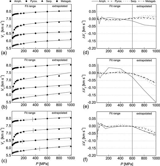
Results of curve fit and velocity extrapolation according to (a) eq. (1), (b) eq. (2) and (c) eqs (3a)/(3b). Symbols refer to experimental data, approximated functions are given by solid lines. Experimental error bars are smaller than symbol size (60.1 ∼ 80.0 × 10⁻³ km s⁻¹), for particular error magnitudes refer to Table 1. In diagram (c), critical pressures P_c—corresponding to the transition from non-linear to linear behaviour—are indicated by vertical bars. Diagrams (d)–(f) illustrate particular errors ΔV=V_exp−V_fit of the fits and of the extrapolated velocity trends.

Open in new tabDownload slide

Table 1

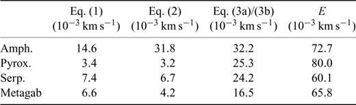
RMS errors of the fits to the Madison data according to eqs (1), (2) and (3a)/(3b) considering the pressure range ≥ 600MPa. Parameter E refers to the experimental error at P = 600MPa assuming a bulk error of 1 per cent.

Open in new tabDownload slide

Significant differences of RMS errors for the amphibolite sample let us conclude that eq. (1) generally offers the better results. It best matches the rapidly changing velocity gradients dV/dP at low pressures. Note that the fit to the V_P of the amphibolite sample is characterized by maximum bulk errors, indicating that its velocity trend is hard to describe by any relation. The critical pressure P_c of eqs (3a)/(3b) is located within the data range (183 MPa ≤P_c≤ 470 MPa; Fig. 2c), demonstrating that, in a statistical sense, the onset of linear velocity increase with pressure occurs at rather low pressure. Comparing the ‘intrinsic’ parameters of eqs (2) and (3b), the difference between zero pressure velocities a₂ and d₃, respectively, is usually ≤1 per cent, except for the amphibolite sample where the 2 per cent difference between particular parameters exceeds the experimental error of 1 per cent (Table 2). Pressure derivatives b₂ and e₃ differ significantly more, in case of the amphibolite sample, parameter b₂ is twice parameter e₃.

Table 2

Comparison of the ‘intrinsic’ parameters of the fits to the Madison data according to eqs (2) and (3b).

Open in new tabDownload slide

The distribution of fit errors, ΔV(P) =V_exp(P) −V_fit(P), delivers additional information. Mostly, the error functions do not scatter statistically around the zero line but show consistent deviation to positive or negative values over a wide pressure range (Figs 2(d)–(f)). This behaviour is most prominent for the fit of eq. (2) to the amphibolite sample, where the errors are positive in the range 100 MPa < P < 500 MPa and become negative above P= 600 MPa (Fig. 2e). Generally, eq. (1) offers the smallest error magnitudes within the fit range (|ΔV₁| < 0.04 km s⁻¹; |ΔV₂| < 0.07 km s⁻¹; |ΔV₃| < 0.09 km s⁻¹).

Extrapolated velocity trends to 1000 MPa are different for all relations, and this holds true for trends and magnitudes of ΔV_i as well. The main observation is that extrapolated velocities are consistently too high or too low compared to the experimental velocities. In case of eq. (1), calculated velocities are mostly too small (ΔV₁ < 0.03 km s⁻¹ at P= 1000 MPa), except for the amphibolite sample where the calculated velocity is too high (ΔV₁=−0.05 km s⁻¹; Fig. 2d). In case of eqs (2) and (3b), extrapolated velocities are generally too high. Mostly, ΔV₂ is smaller than −0.1 km s⁻¹ at P= 1000 MPa, but approaches −0.2 km s⁻¹ for the amphibolite sample, which is characterized by the poorest fit (Fig. 2e). Magnitudes of ΔV₃ are close together and do not exceed −0.07 km s⁻¹ at P= 1000 MPa (Fig. 2f). As a consequence of consistent deviation of extrapolated velocities to higher velocities, estimated pressure gradients b₂ (eq. 2) and e₃ (eq. 3b) are too large. From experiments to 3 GPa, Christensen (1974) derived pressure gradients of about 0.15 ∼ 0.16 × 10⁻³ km s⁻¹ MPa⁻¹ for two pyroxenite samples. These are two to three times smaller than gradients obtained from eqs (2) and (3b) (Table 2) and, therefore, support this observation.

Although eq. (1) best extrapolates the velocity trends, estimation of the ‘intrinsic’ velocity trend from the above denoted monotonous growth of exponential functions may be erroneous due to observed systematic errors. Eq. (2) fails, because the ‘intrinsic’ trend, a₂+b₂ P, is hard to separate from non-linear low-pressure measurements with sufficient accuracy, leading to systematic errors of extrapolated velocity trends as well. Eqs (3a)/(3b) fail because the critical pressure P_c is constrained to be smaller than P_max of the fit data. Systematic deviations at pressures >P_max are interpreted such that, in fact, P_c exceeds P_max. In summary, observed consistent discrepancies between experimental and extrapolated velocities indicate that all relations are unsuitable for reliable extrapolation of pressure–velocity trends to high pressures, in particular, for reliable evaluation of ‘intrinsic’ velocity trends from low-pressure measurements.

4 The Alternative Approach

Our approach intends to evaluate the ‘intrinsic’ velocity trend from all shapes of the velocity—pressure function, avoiding in particular systematic errors, which disqualify the relations discussed above. We propose to refine the ‘intrinsic’ terms obtained by one of eqs (2) or (3b) in a subsequent procedure. The optimization should be solely dependent on the refinement procedure itself, that is, the basic equation to be applied should avoid restrictions for the ‘intrinsic’ terms. This requirement is met by eq. (2) only.

We take advantage of the observation that magnitudes of the ‘intrinsic’ parameters—a₂ and b₂ in case of eq. (2)—change in dependence on maximum pressure P_max applied in the fit (Greenfield & Graham 1996). Non-linear increase (a₂) or decrease (b₂) were observed, with both parameters approximating a constant value at pressure much higher than ‘crack closure pressure’. This behaviour is a clear indication that the ‘intrinsic’ velocity trend cannot be reproduced accurately from low-pressure experiments, however, observed non-linear convergence can be used to obtain better estimates of parameters a₂ and b₂ from these measurements.

First, independent fits to successively increasing maximum pressures P_max were performed to obtain trends of parameters a₂ and b₂ against the P_max. The number of data from the Madison experiments is too small for that purpose, hence, P-wave data measured on amphibolite and gneiss sample at the triaxial pressure device at Institut für Geowissenschaften, Kiel, Germany (Kern et al. 2002) applying small pressure increments (ΔP= 12 MPa for P≤ 50 MPa; ΔP= 25 MPa for P≤ 100 MPa; ΔP= 50 MPa for P > 100 MPa; Fig. 3) are used to perform the fits to maximum pressures of P_max= 304–355, 406–457, 508–560 and 611 MPa. Hornblende (82 per cent) is the main constituent of the amphibolite sample, the gneiss sample consists of quartz (38 per cent), phyllosilicates (34 per cent), plagioclase (25 per cent) and minor potassic feldspar (Ullemeyer et al. 2006, samples TW11 and TW9 therein). Due to crystallographic preferred orientation of hornblende, quartz and phyllosilicates, and due to anisotropy of pore space distributions, P-wave trends of both samples are different for the principal directions X, Y, Z of the structural reference frame, in which the measurements were performed (Ullemeyer et al. 2006). RMS errors E_fit of the individual fits range from 6.7 ∼ 32.9 × 10⁻³ km s⁻¹ for the amphibolite sample and from 7.3 ∼ 14.6 × 10⁻³ km s⁻¹ for the gneiss sample, bulk experimental errors E include 65.7 ∼ 68.3 × 10⁻³ km s⁻¹ and 57.0 ∼ 63.8 × 10⁻³ km s⁻¹, respectively (refer to Table 3 for details). The error magnitudes are similar to the fits to the Madison data, hence, the same conclusions concerning goodness of the fits and experimental errors are valid.

Figure 3

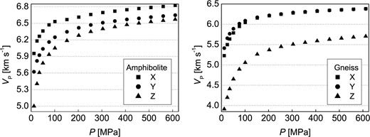
Low pressure (P_max = 611 MPa) P-wave measurements in three perpendicular sample directions X, Y, Z. The data are used for independent fits to various maximum pressures (304 ≤P_max≤ 611 MPa) and subsequent refinement of parameters a₂ and b₂.

Open in new tabDownload slide

Table 3

RMS errors of the fits to the Kiel data. E: experimental error at P = 611 MPa; E_fit: error range of the fits to various maximum pressures according to eq. (2); E_ref : error of the refinement fits to parameters a₂ and b₂ according to eq. (4).

Open in new tabDownload slide

Secondly, observed convergence of parameters a₂ and b₂ is used to describe particular trends against the P_max independently from each other by means of an exponential function,

4

(A, B, C are coefficients of the function, y is one of parameters a₂ and b₂, determined by unweighted fits to various maximum pressures according to eq. (2)). The point of convergence, A, is expected to represent the ‘true’ magnitudes of parameters a₂ and b₂, respectively. Since parameter a₂ increases with P_max, the exponential function is inverse (B > 0), in case of parameter b₂ the function decays (B < 0). RMS errors E_ref of the refinement fits range from 0.48 ∼ 1.19 × 10⁻³ km s⁻¹ (a₂) to 0.38 ∼ 4.8 × 10⁻⁶ km s⁻¹ MPa⁻¹ (b₂) (Table 3), demonstrating very close agreement of the model function to the data and suitability of eq. (4) for the refinement from the statistical side of view.

As it was predicted, parameters a₂ and b₂ change in dependence on maximum pressure of the fits (Fig. 4, symbols), proving that a maximum pressure of 611 MPa in the experiments is too low to determine the ‘intrinsic’ parameters accurately by means of curve fit according to eq. (2). The extent of changes is different, compare trends of b₂ of the amphibolite sample as an example. Most trends determined in such a way are non-linear and tend to some value, but few trends appear to be linear, for example, X direction of the amphibolite sample (Fig. 4). Nevertheless, eq. (4) was applied to all data sets and, always, convergence of the extrapolated trend was observed. Deviations of the approximated points of convergence and corresponding values from the fits to P_max= 611 MPa may be small (e.g. X direction of the gneiss sample: A= 6.19 km s⁻¹, a₂ (P= 611 MPa) = 6.14 km s⁻¹; Fig. 4), but very large discrepancy holds true as well (X direction of the amphibolite sample: A= 7.84 km s⁻¹, a₂ (P= 611 MPa) = 6.51 km s⁻¹; Fig. 4). Obviously, the latter estimate of parameter a is erroneous, which is confirmed by the large error assigned to A (±36 per cent ≡±2.79 km s⁻¹). Large error concerning parameter A=b₂ is also observed for Y direction of the gneiss sample (±20 per cent ≡±0.038 10⁻³ km s⁻¹ MPa⁻¹; Fig. 4). In both these cases, the results of refinement are doubtful and should not be interpreted, whereas small errors (frequently <1 per cent) indicate statistically reliable results.

Figure 4

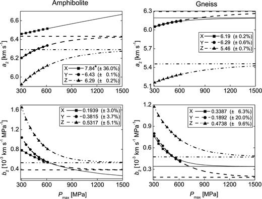
Magnitudes of the ‘intrinsic’ parameters a₂ and b₂ in dependence on maximum pressure P_max in independent fits to the data shown in Fig. 3 (symbols). Extrapolated trends of parameters a₂ and b₂ to 1500 MPa applying eq. (4) are indicated by lines. Points of convergence A (the optimized parameters a₂ and b₂) are given in the legend and illustrated by horizontal lines in the graph. Percent values indicate errors of parameter A. * not shown for better scaling (top left graph).

Open in new tabDownload slide

5 Discussion

Experiments to very high pressures with an adequate number of data in the low-pressure range would have been required to verify the results of parameter refinement directly. Suitable equipment is currently not available. The unique data set of Christensen (1974) fails, because the number of data is too small to perform independent fits to various maximum pressures in the low-pressure range. Thus, reliability of our approach cannot be proven by experimental data, however, several observations indicate that the refined ‘intrinsic’ velocity trends approximate the ‘true intrinsic’ velocity trends better as the trends obtained via eqs (2) and (3a)/(3b) do. Since eq. (2) provides the basis of our refinement procedure, the discussion focuses on the comparison of the ‘intrinsic’ velocity trends derived from eqs (2) and (4), but the results of eqs (3a)/(3b) will be discussed as well. In the following, refinement runs with large error magnitudes of parameter A—the amphibolite X and gneiss Y sample directions—were avoided.

Visual inspection of the extrapolated trends presented in Fig. 4 indicates that most cracks are actually closed at pressures P_max = 1000 ∼ 1500 MPa, because changes of gradients become small within this pressure interval. This observation holds true for both samples and is confirmed by the experiments of Christensen (1974) on mantle rocks and by the findings of Greenfield & Graham (1996). Such conformity implies that optimized parameters a₂ and b₂ are not completely unfounded and, due to convergence of eq. (4), the refinement leads to better estimates of particular parameters anyway.

Direct evidence for improved ‘intrinsic’ velocity trends can be derived from their relation to the experimental data. In agreement with theory (‘intrinsic’ velocity represents an upper limit of possible velocities), the optimized ‘intrinsic’ functions never intersect the experimental functions as the ‘intrinsic’ functions estimated by means of eq. (2) do and, accordingly, the ‘crack closure pressure’P_c locates beyond the data range (Fig. 5). The unrealistic consequence of such intersection is that the functions do not converge but diverge at higher experimental pressure. This is best visible for Z direction of the amphibolite sample (Fig. 5), where the ‘intrinsic’ function intersects the experimental function over a wide pressure range of 200 ∼ 450 MPa. Always, eq. (2) leads to lowest ‘intrinsic’ velocities at zero pressure and to maximum ‘intrinsic’ gradients, the maximum discrepancy between gradients approaches factor two (Table 4). Obviously, gradients b₂ are too large, which is confirmed by the visual impression of discontinuity at P_max (Fig. 5). Furthermore, a₂ is clearly too small. The effect is twofold (i) estimated ‘intrinsic’ velocities for P= 1500 MPa are the highest, the maximum deviation to our refined velocity estimate is 0.23 km s⁻¹ (Fig. 5, Table 5) (ii) the area representing the crack-induced velocity decrease at low pressures (Fig. 1) decreases significantly, that is, quantification of the crack influence especially at very low pressure is falsified. All these observations confirm that plain exponential functions are unsuitable to describe the non-linear part of the velocity—pressure function accurately, with the consequence that the ‘intrinsic’ velocity trend cannot be determined correctly from low-pressure experiments by means of eq. (2).

Figure 5

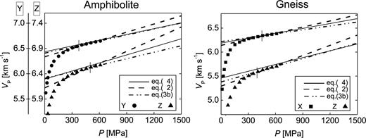
Comparison of ‘intrinsic’ velocity trends, derived from optimized parameters a₂ and b₂ according to eq. (4) (solid lines), from fits according to eq. (2) (dashed lines), and from fits according to eq. (3b) (dash-dotted lines). Symbols indicate experimental data. Sample directions X of the amphibolite and Y of the gneiss are avoided due to large errors of parameter fit (see text for discussion). Critical pressures P_c belonging to eq. (3b) are indicated by vertical bars. For better visualization, scaling of the diagram at the left is different for Y and Z direction.

Open in new tabDownload slide

Table 4

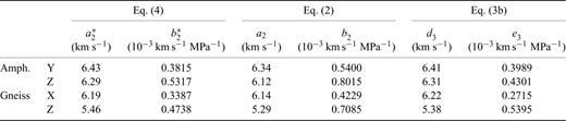
Comparison of the ‘intrinsic’ parameters of the fits to the Kiel data according to eqs (4) (a^*₂, b^*₂ : optimized parameters a₂ and b₂), eq. (2) (parameters a₂ and b₂) and eq. (3b) (parameters d₃ and e₃).

Open in new tabDownload slide

Table 5

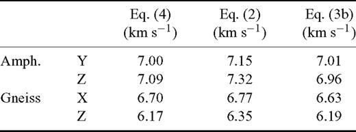
Extrapolated ‘intrinsic’ velocities at P = 1500MPa.

Open in new tabDownload slide

Occasionally, the gap between the refined ‘intrinsic’ velocity trend and the experimental velocities at maximum experimental pressure appears to be rather large (Z directions of both samples; Fig. 5), implying that the ‘crack closure pressure’ locates at very high pressure. Whereas the experimental data set represents a lower boundary of possible ‘intrinsic’ velocity trends, no upper boundary can be inferred from the data and used to check plausibility of this observation. However, some fabric characteristics indicate that the velocity gap at P_max is realistic. The Z direction of both samples is perpendicular to the predominant foliation, which generally represents the most prominent anisotropy plane of rocks. Anisotropic pore space distributions with the highest anisotropy parallel to the foliation normal were observed (Ullemeyer et al. 2006), leading to more pronounced velocity decrease with decreasing pressure compared to the other sample directions.

Eqs (3a)/(3b) constrain the ‘intrinsic’ function to fit the experimental function at pressures P > P_c. Particular critical pressures P_c of 365/494 MPa for the amphibolite sample and 383/471 MPa for the gneiss sample are known to be too low, that is, for P > P_c the experimental function is essentially non-linear and the ‘true intrinsic’ function locates above the modelled one. The ‘intrinsic’ pressure derivative e₃ is expected to be smaller and the zero pressure velocity d₃ to be higher. Since, always, e₃ is less than b₂ and d₃ exceeds a₂ (Table 4, Fig. 5), particular trends are closer to the ‘true intrinsic’ velocity trend. From this point of view eqs (3a)/(3b) are superior to eq. (2). On the other hand, dependent on P_c, the linear fits are based on few experimental data covering a small pressure interval only (see Fig. 5). Hence, statistical relevance of the correlation coefficient r², which is the criterion for linearity of the velocity trend, is poor. Despite rather small experimental errors of about 60 × 10⁻³ km s⁻¹ (Table 3), reliability of the ‘intrinsic’ function becomes worse the higher the critical pressure P_c.

6 Conclusions

We conclude that all relations for the approximation of velocity–pressure trends discussed above are unsuitable for doubtless prediction of the ‘intrinsic’ velocity–pressure trends from low-pressure experiments. This holds true despite the observation that some relations describe most velocity–pressure trends sufficiently well within the measuring range. The relation proposed by Pros et al. (1998) fails in describing the non-linear part of the velocity–pressure equation with sufficient accuracy, which finds its expression in the obviously unrealistic intersection of the ‘intrinsic’ velocity trend with the experimental data. Such intersection was observed for all measurements we ever tried to approximate by means of eq. (2), for this reason, we cannot recommend use of this approach for the evaluation of the ‘intrinsic’ velocity trend.

Due to the assumption that the ‘crack closure pressure’ is lower than maximum pressure in the experiment, the approach of Wang et al. (2005) avoids intersection of the model functions and the experimental functions. The approach is, therefore, superior to the approach of Pros et al. (1998). However, the true ‘crack closure pressure’ is clearly located beyond the maximum pressures sampled. It may be assumed that the approach leads to increasingly better results the smaller the critical pressure P_c estimated by means of eqs (3a)/(3b), on the other hand, there is no independent criterion to decide whether the predicted ‘intrinsic’ velocity trends are within acceptable errors or not.

Since limiting constraints concerning the ‘crack closure pressure’ are avoided, and due to the fact that unrealistic intersection of the ‘intrinsic’ function and the experimental function can be prevented, our refinement procedure clearly offers a better approximation of the ‘true intrinsic’ function as both the other approaches do. Indeed, uncertainty about obtained trends persists, as the positive proof cannot be provided due to lacking experiments to sufficiently high pressures. In addition to the examples presented, the procedure was applied to a large number of cube sample measurements. Convergence of eq. (4) was observed in all cases, however, the error level assigned to the approximated point of convergence was frequently inacceptable. In summary, we conclude that our approach offers an approvement of already existing approaches, provided that the errors are evaluated carefully and obtained ‘intrinsic’ velocity trends are judged critically because of missing experimental verification.

Acknowledgments

We are grateful to Till Popp and Detlef Schulte-Kortnack for the cube sample measurements. Qin Wang kindly provided her MATLAB program for curve-fitting. The constructive reviews by Tom Brocher and David Mainprice were helpful to improve the manuscript significantly. This research was supported by the German Federal Ministry of Education and Research through grant 03DU03FB.

References