


Summary
We develop a new method to estimate geometries of dipping seismic velocity discontinuities from common conversion point stacking of receiver functions. The multistage fast-marching method is applied to the ray tracing with refraction at dipping interfaces. Although geometry of interfaces dipping at 30°–70° cannot be correctly estimated with a 1-D velocity model, it can be correctly estimated when refraction at dipping interfaces is taken into account. We apply this method to synthetic and observed data and confirm that geometries of dipping interfaces are successfully estimated. This method will contribute to revealing the structures beneath subduction zones where dipping interfaces exist.
1 Introduction
The receiver function (RF) technique (Langston 1979) is a useful method for detecting phases converted at seismic velocity discontinuities in a teleseismic coda. The depth of a discontinuity can be estimated from the lag time of arrivals between a P wave and a converted phase with an assumed velocity model. The geometries of the continental Moho or of the oceanic Moho of subducting slabs have been detected with RF imaging (e.g. Yamauchi et al. 2003). In many cases, refraction of seismic waves at dipping interfaces has not been taken into account when RFs are stacked. Seismic rays traced assuming horizontal interfaces would have different paths from those of true rays that pass through dipping interfaces. Refraction of seismic waves at dipping interfaces should be taken into account for accurate estimation of interface geometry.
We stack RFs, which are synthesized with a velocity model containing dipping interfaces, and show the error in the interface geometry estimated with a horizontally layered 1-D model of ak135 (Kennett et al. 1995). To reduce the error, we develop a new method for stacking RFs using the multistage fast-marching method (FMM, de Kool et al. 2006).
2 Synthesizing Receiver Functions for a Velocity Model with Dipping Interfaces (Slab Model)
2.1 Assumed velocity structure
We assume a model, which has widths of 5° in both latitude and longitude (the centre of the model is at latitude 32.5°) and a thickness of 315 km (0–315 km in depth). The model contains a slab subducting towards the west and we show a part of the model in Fig. 1. We call this model the ‘Slab Model’. The model contains five interfaces dividing the model region into six parts. The seismic velocities of the slab mantle are 105 per cent of those of ak135. This velocity anomaly of the slab mantle is consistent with regional tomographic studies in Japan (e.g. Nakajima et al. 2001; Nakajima & Hasegawa 2007). P- and S-wave velocities of the subducting oceanic crust are assumed as 86 per cent and 88 per cent of those of ak135, respectively, so that the assumed velocity contrast at the oceanic Moho is the same magnitude as the velocity contrast at the Moho in ak135. The other regions have the same velocities as the ak135 model. The slab is assumed to be bending, and the dip angle changes from 30° to 70° around a depth of 80 km (Fig. 1). We assume the seismic velocity structure extends in the latitude direction. In this respect, our modelling is 2.5-D.
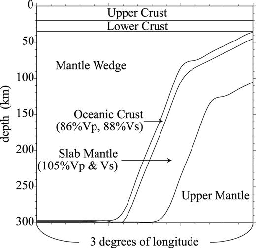
The assumed seismic velocity structure, in which a high-velocity slab mantle with a low-velocity oceanic crust is subducting (Slab Model). Assuming this structure, we synthesize RFs with the Gaussian Beam Method. This structure is modelled after the Philippine Sea slab subducting beneath Kyushu, southwest Japan.
2.2 Synthetic teleseismic events and seismic stations
To select hypocentres and the components of RFs, which are suitable for detecting the assumed interfaces, we examine how RF amplitudes are affected by dipping interfaces assuming a simple half-space model with two layers. S-wave velocities of the upper and lower layers are assumed to be 4.0 km s−1 (Vp= 6.9 km s−1) and 4.5 km s−1 (Vp= 8.1 km s−1); 4.5 km s−1 and 8.1 km s−1 are the same as the S- and P-wave velocities of the uppermost mantle in the ak135 model, respectively. The interface is assumed to exist at a depth of 70 km beneath a station and to dip at 10°, 20° or 30° towards the west. We synthesize teleseismic waves whose ray parameters are 0.042 s km−1 (corresponding epicentral distance of 90°) with generalized ray theory (Helmberger 1974), and calculate RFs from the synthetic waveforms with the extended-time multitaper method (Helffrich 2006) improved by Shibutani et al. (2008). In Fig. 2, we show synthetic RFs, on which Ps phases converted at the assumed interface appear at 6–8 s. Cassidy (1992) also examined dipping layer effects on RFs. Amplitudes of Ps phases on our synthetic RFs (Fig. 2) have the same dependence on backazimuths as those of his study.
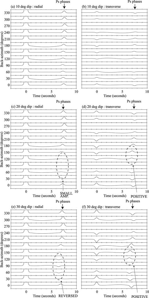
RFs synthesized with generalized ray theory assuming the two-layered half-space model. In each plate, RFs are shown in each 30° of backazimuth. RF amplitudes from –0.1 to 0.1 are shown to make Ps converted phases more clear. (a and b) Radial and transverse RFs synthesized assuming the interface dips at 10°; (c and d) those at 20°; (e and f) those at 30°.
If the dip angle of the interface is 10° (Fig. 2a), Ps phases on radial RFs have larger positive amplitude than those on transverse ones. The amplitude of radial RFs with downdip backazimuth (around 90°) is very small when the interface dips at 20° (Fig. 2c), and their polarity is reversed when the interface dips at 30° (Fig. 2e). Since the polarity of a radial RF with a larger ray parameter would not be reversed until the interface dips more steeply, radial RFs are suitable for geometric estimation of interfaces dipping at less than 20°. However, we should not use radial RFs with downdip backazimuth for geometric estimation of interfaces dipping at larger than 20°, because some of them would disturb the estimation.
In contrast, the polarity of transverse RFs does not change depending on the dip angle of the interface, although it changes depending on backazimuth (Fig. 2b, d and f). Therefore, radial RFs with updip backazimuth or transverse RFs with the restricted backazimuth should be used to detect interfaces dipping at larger than 20°.
If an interface dips at larger than 50°, some teleseismic waves with updip backazimuth impinge nearly parallel to the interface. Consequently, it is difficult to detect the interface. The incident angle of a teleseismic P wave with a ray parameter of 0.08 s km−1 (corresponding epicentral distance of 30°) is always larger than 40° in the mantle if a horizontally layered structure (ak135) is assumed. Therefore, neither radial nor transverse RFs with updip backazimuth should be used to detect interfaces dipping at larger than 50°.
Because interfaces in the Slab Model are assumed to dip at 30°–70° towards the west, only transverse RFs which come from the southeast or the northeast should be used for detecting them. We construct the synthetic waveforms arising from nine synthetic teleseismic events whose backazimuths from the modelled region are 105°, 135° and 165° and whose epicentral distances from the region are 40°, 60° and 80°, respectively. Hypocentres of these events are assumed to be on the ground surface. Teleseismic rays impinge from the southeast onto the slab subducting towards the west.
26 stations are assumed to be on an E–W line spaced evenly at a separation of 0.1° longitude. The locations of the synthetic seismic stations are aligned perpendicularly to the strike of the assumed subducting slab.
2.3 Calculating RFs for the Slab Model
We calculate RFs from teleseismic waveforms synthesized with the Slab Model and the synthetic event/station distributions. A code constructed by Sekiguchi (1992) and modified by Hirahara et al. (2007) is used for synthesizing waveforms with the Gaussian Beam Method (Červený 1985). To calculate RFs, we use the extended-time multitaper method (Helffrich 2006) improved by Shibutani et al. (2008).
3 Stacking Receiver Functions with a 1-D Velocity Model (AK15)
We migrate these synthetic transverse RFs to the depth domain with the ak135 velocity model, and project them on a section which consists of 0.02° in longitude by 2 km in depth cells and is parallel to latitude lines (Fig. 3). When two or more RFs are projected on the same cell, the amplitudes are averaged. Ps phases converted at discontinuity interfaces dipping towards the west with upward decreasing velocity, produce positive peaks on transverse RFs with backazimuths of 105°–165° (Figs 2d and f), while those converted at discontinuity interfaces with upward increasing velocity produce negative peaks.
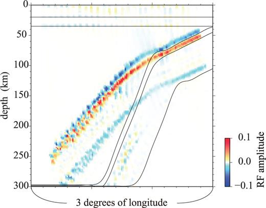
A vertical section, which is constructed by stacking transverse RFs with a 1-D velocity model (ak135). These transverse RFs are synthesized with the Gaussian Beam Method by assuming the Slab Model shown in Fig. 1. The colour bar shows the scale of RF amplitude. Positive (negative) peaks of these transverse RFs are produced by interfaces dipping towards the west with upward decreasing (increasing) velocities. Solid lines indicate the assumed interfaces of the Slab Model shown in Fig. 1.
In Fig. 3, peaks of RFs indicate three dipping interfaces. The top and the bottom of the slab are indicated by negative peaks (blue), and the oceanic Moho is indicated by positive peaks (red). The interface geometry estimated from the RF peaks is different from the assumed geometry indicated by solid lines in Fig. 3. The cause of the difference is that the RFs are stacked with ak135 in spite of the fact that those RFs are synthesized with the Slab Model shown in Fig. 1. Therefore, we now investigate how to take into account refraction of seismic rays at dipping interfaces to improve the geometric estimation.
4 Stacking Receiver Functions with the Multistage FMM
We stack RFs taking account of refraction using 3-D traveltime fields calculated with the multistage FMM. We use a grid model that has widths of 3° in both latitude and longitude and a thickness of 301 km (from 1 km above sea level to 300 km below sea level), with a grid spacing of 0.02° in the horizontal directions and of 2 km in depth to calculate traveltime fields.
First, we use the Slab Model as a velocity structure. Traveltime fields of P wave propagated upwards from the synthetic teleseismic events and those of S wave propagated downwards from the synthetic stations are calculated with the multistage FMM (Figs 4a and b). With these traveltime fields, for each pair of a teleseismic event and a station, the lag time of arrivals between the teleseismic P wave and a Ps wave converted at a node and scattered to the station are obtained by subtracting the P-wave arrival time at the station from the sum of the P- and S-wave traveltimes to the node. An example of a lag time field is also shown in Fig. 4(c). To follow Snell's law, we select nodes in which the P-wave slowness vector component that is parallel to the nearest interface is opposite in direction and equal in magnitude to the corresponding component of S-wave slowness vector (Figs 4d and e). With the selected nodes and their lag times, the amplitudes of each transverse RF are plotted in the model region. When two or more RFs are plotted in the same node, the amplitudes are averaged. A section of the stacked RFs is shown in Fig. 5(a). The assumed interfaces are correctly estimated.
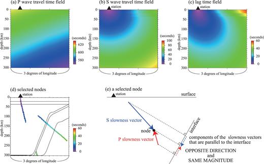
(a) Traveltime field of a teleseismic P-wave generated by a synthetic hypocentre whose backazimuth and distance from the modelled region are 135° and 60°, respectively. (b) Traveltime field of an S-wave propagated from the station indicated by a triangle. (c) Lag time field of arrivals at the station between teleseismic P wave and S wave converted at each node. (a), (b) and (c) are vertical sections beneath the E–W array of the synthetic seismic stations. (d) Nodes selected as conversion points projected on a vertical plane parallel to latitude lines. (e) A schematic explanation for a selected node. A black circle indicates a node that is selected as a conversion point. Red and blue solid arrows indicate the P- and S-wave slowness vectors at the node, respectively. Red and blue dashed arrows indicate components parallel to the interface of the P- and S-wave slowness vectors, respectively.
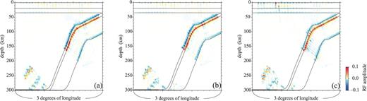
(a) RF section stacked with the multistage FMM by assuming the Slab Model. (b) RF section stacked with the multistage FMM by assuming ak135 and dipping interfaces of the Slab Model. (c) RF section with RFs synthesized with a velocity model whose mantle wedge has 5 per cent lower seismic velocities than the Slab Model's, stacked with the multistage FMM by assuming ak135 and dipping interfaces of the Slab Model.
In Fig. 5(b), we show an RF section which is constructed by assuming the ak135 velocity model and interface geometry of the Slab Model (shown in Fig. 1). In this case, although the velocity values are the same as those of ak135, which is different from the Slab Model, the P-to-S conversion occurs at interfaces, which are not horizontal but dipping at the same angle as the nearest interface in the Slab Model. The estimation of interface geometry is also successful and a small error contained in the RF section in Fig. 5(b) is not a practical issue. Nakajima et al. (2001) and Nakajima & Hasegawa (2007) indicated that a low-velocity anomaly of about 5 per cent exists in the mantle wedge, in Japan. We migrate RFs synthesized with another velocity model which has 5 per cent lower Vp and Vs in the mantle wedge than the Slab Model and the same velocities as the Slab Model in the other layers, and obtain an RF image (Fig. 5c). The error of interface geometry estimated from this image is also negligibly small. These findings imply that estimation of dip angles of interfaces are critical for estimating their geometries, and RF images are not strongly affected by velocity anomaly expected to exist in subduction zones. In the following, therefore, we stack RFs with models, which have arbitrary interfaces and the same velocities as ak135 at the nodes.
5 Estimation of Interface Geometry
When we apply our approach to the estimation of subduction zone structure from observed data, we do not know the accurate interface geometry at the outset. Therefore, we develop a method to estimate the geometry iteratively by assuming approximate dip directions to restrict the backazimuthal range of teleseismic events.
At the first iteration, we stack RFs by assuming only the ak135 model with no dipping interfaces and make the first estimation of the geometry. In each of the following iterations, we use the previously estimated geometry of dipping P-to-S conversion interfaces to calculate a new stack.
We apply this method to the RFs synthesized with the Slab Model and synthetic event/station distribution. In Fig. 6, we show synthetic RF sections produced in each iteration. Fig. 6(a) shows a RF section with RFs stacked assuming just the Conrad and the continental Moho. Figs 6(b) and (c) show RF sections with RFs stacked assuming the dipping interfaces estimated from Figs 6(a) and (b) (solid black lines in each section), respectively. RF peaks in Fig. 6(c) correspond to the purple lines which indicate the interfaces of the Slab Model and the interface geometry is successfully estimated.
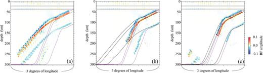
(a) RF section stacked with ak135. (b) and (c) RF sections stacked with ak135 and interfaces estimated from the section (a) and (b), respectively. Black lines indicate the interfaces assumed to stack RFs. Purple lines indicate interfaces of the Slab Model.
6 Application to Observed Data
We apply this method to estimate the geometry of the Philippines Sea slab beneath the Kyushu district, southwest Japan.
We use 9718 waveforms from 255 teleseismic events (backazimuth: 118°–178°, epicentral distance: 30°–90°, magnitude greater than 5.5, origin time: 1996 August–2009 February, shown in Fig. 7a) observed at 55 stations of Hi-net (Obara et al. 2005) established by the National Research Institute for Earth Science and Disaster Prevention (NIED) and at 31 stations of the J-array (Morita 1996) established by the Japan Meteorological Agency (JMA), Kyushu University and Kagoshima University (Fig. 7b).
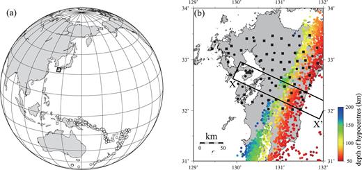
(a) Epicentral distribution. Circles indicate epicentres of teleseismic events that we analyse. We stack RFs beneath the box. (b) Station distribution. Squares and black circles indicate Hi-net and the J-array stations, respectively. Coloured circles indicate hypocentres of earthquakes determined by JMA which occurred deeper than 50 km.
We calculate transverse RFs with the extended-time multitaper method (Helffrich 2006) improved by Shibutani et al. (2008) and exclude frequencies higher than 0.3 Hz. We stack these RFs in the region at latitudes 32°–33.5° north, longitudes 129°–132° east and depths from 1 km above sea level to 300 km below sea level, with the method explained in Sections 4 and 5.
First, RFs are stacked by assuming two horizontal interfaces (the Conrad and the Moho at depths of 20 km and 35 km, respectively), and the RF section along X–X′ beneath the box in Fig. 7(b) is shown in Fig. 8(a). Positive peaks of transverse RFs, which are expected to indicate the oceanic Moho of the Philippine Sea slab, can be seen in Fig. 8(a). The positive peaks do not correspond to the hypocentres of intermediate-depth earthquakes in the portion deeper than 70 km, and this is caused by the fact that refraction at dipping interfaces of the Philippine Sea slab is not taken into account.
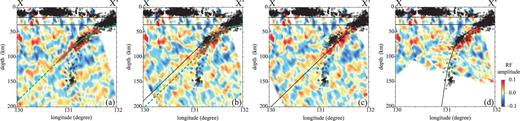
RF sections X–X′ in Fig. 7(b). In each section, black lines indicate interfaces which we assume for stacking RFs. Solid green lines indicate interfaces estimated from RF peaks and dashed green lines indicate interfaces which are arbitrarily extended. (a) RF section stacked with ak135. Positive peaks, which are expected to indicate the oceanic Moho, separate from hypocentres of intermediate-depth earthquakes at depths greater than 80 km. (b) and (c) RF sections stacked with ak135 and estimated interfaces indicated by solid and dashed green lines in (a) and (b), respectively. In (c), positive peaks expected to indicate the oceanic Moho correspond to the interface (indicated by the black line) assumed for stacking these RFs and the interface geometry is successfully estimated, although positive peaks are not detected at depths greater than 90 km. These positive peaks also correspond to hypocentres of intermediate-depth earthquakes. (d) RF section stacked with ak135 and an interface which is estimated as a top of the slab from seismic activity. Positive RF peaks are not detected at depths greater than 90 km, even if we stack RFs by assuming an interface whose geometry corresponds to hypocentres of intermediate-depth earthquakes.
Next, we stack RFs again by assuming an additional interface. The additional interface is estimated from the first stacking indicated by solid and dashed green lines in Fig. 8(a). The second and the third RF images are shown in Figs 8(b) and (c), respectively. In the third image (Fig. 8c), the positive peak corresponds to the assumed interface, and its geometry has been estimated. The positive peak also corresponds to a swarm of intermediate-depth earthquakes, which implies that the geometry of the oceanic Moho of the Philippine Sea slab has been successfully estimated.
Ps phases converted at the oceanic Moho deeper than 90 km are not detected despite the fact that the swarm of intermediate-depth earthquakes extends down to 160 km in depths. This does not mean that this iterative estimation fails to detect the geometry of the oceanic Moho. Even if we stack RFs by assuming the Conrad, the Moho and an additional interface (the black curved line in Fig. 8d) which is estimated as a top of the slab from seismic activity, the obtained RF section also does not have positive RF peaks around the assumed interface beneath 90 km. Therefore, we conclude that the oceanic Moho beneath 90 km has too small a velocity contrast to be detected with RFs.
7 Discussion
We have shown with both synthetic and observed data that our new method correctly detects dipping interfaces, which are not detected by a conventional method with a 1-D model. This new method will reveal the geometry of subducted slabs, as we have shown the case of the Philippine Sea slab beneath Kyushu in Section 6, which will contribute to understand structures and water transportation in the upper mantle of subduction zones. Kawakatsu & Watada (2007) interpreted positive RF peaks along the Wadati–Benioff zone beneath northeastern Japan in their RF section as the bottoms of the hydrated oceanic crust and the serpentinized mantle wedge. Beneath the central part of the Kyushu district, it is expected from the constructed RF image (Fig. 8c) that the bottom interfaces of the hydrated layers exist at the depths down to 90 km and the fluid is expected to be conveyed down to this depth along the Philippine Sea slab.
Kirchhoff migration of RFs (e.g. Sheehan et al. 2000; Boyd et al. 2007) can also estimate geometries of dipping interfaces. In the method, S waves are assumed to be scattered to a station at all nodes, and RF amplitudes are assigned to the nodes based on the arrival time difference between the teleseismic P wave and the scattered S wave. In contrast, in our method we select nodes where teleseismic P waves are converted to S waves with satisfying Snell's law at dipping interfaces, and assign RF amplitudes on the selected nodes. Therefore, we can more adequately stack RF peaks, which are derived from Ps converted phases.
As described in Section 2, we should use RFs with adequate horizontal (radial or transverse) component and backazimuth depending on the dip angle and dip direction of the interfaces to be detected. In some cases, it is difficult to select RFs to stack. For example, when the dip angle of the interface varies from gentle angle (<20°) to steep angle (>50°), transverse RFs would disturb the estimation of the gently dipping portion, while radial RFs would disturb the estimation of the steeply dipping portion. Or, when the interface has bends in strike direction of subduction, it is difficult to restrict backazimuth of RFs to stack. To detect discontinuity interfaces, which are in any shape, we should develop the method to select RFs whose horizontal component and backazimuth are suitable for detecting them.
Although we have applied this method to synthetic and observed RFs by assuming 1-D velocity model (ak135) and 2.5-D geometry of dipping interfaces, traveltime fields can be calculated assuming 3-D velocity distribution (for example, obtained by regional tomographic studies) and 3-D interface geometry with the multistage FMM. 3-D interface geometry is expected to be accurately obtained with this method.
In conclusion, we have developed a method to stack RFs by considering the refraction of seismic rays at dipping interfaces. Although the geometry of interfaces dipping at 30° and 70° cannot be correctly imaged without considering refraction in P-to-S conversion at dipping interfaces, such a geometry can be correctly estimated when we use this method. This method would enable accurate estimation of 3-D geometry of dipping interfaces, and reveal water transportation beneath subduction zones.
Acknowledgments
We are grateful to Martha Savage for reading this manuscript carefully and giving us many helpful comments. We are also thankful to Anya Reading and an anonymous reviewer for improving this manuscript. We use the multi-stage 3-D fast marching code (de Kool et al. 2006). We use seismic data observed by the NIED, JMA, Kyushu University and Kagoshima University. We also use hypocentral data of JMA. We use GMT (Generic Mapping Tools by Wessel & Smith (1995)) to generate figures. This research has been supported by a Grant-in-Aid for Scientific Research (B) (20340119) from MEXT.
References
