


Summary
A 3-D shear wave velocity model has been established for the lithosphere of southern Tibet through Rayleigh-wave tomography. The teleseismic data are acquired from a 2-D seismic array selected out of the second phase of the Hi-CLIMB project. We first inverted for a 2-D phase velocity model using two-plane-wave tomography approach, and then inverted for the 3-D shear wave velocity model with the 2-D phase velocity model and the map of crustal thickness derived from receiver functions. The results reveal a pervasive low velocity anomaly in the middle crust of the Lhasa block. We interpret this low velocity anomaly as the presence of wholesale mid-crustal channel flow. Prominent low velocity anomalies from the lower crust to the mantle lithosphere are observed along the north–south trending rifts: the Tangra Yum Co rift and the Pumqu Xianza rift. We propose a possible scenario for the formation of these rifts: the entire lithosphere is involved in the early-stage rifting, while the late-stage rifting is restricted in the upper crust. In the non-rift regions, a slab-like high velocity anomaly is traced beneath both the Himalayas and Lhasa block. Combining all the observations, we suggest that the central part of southern Tibet is currently underlain by the broken Indian lower crust and mantle lithosphere.
1 Introduction
The typical example of active continental collision is the Himalayas and Tibetan plateau caused by the collision between the Indian and Asian Plates starting around 55 Ma (Patriat & Achache 1984; Besse et al. 1984). As a result of this collision, the Himalayas are the highest range on the earth and the Tibetan plateau has an average altitude of ∼5000 m and an abnormally thickened crust, approximately twice the average thickness of continental crust. Despite the great efforts made to investigate the Himalayas and Tibetan plateau, the tectonic processes that form the plateau are still under debate. Several candidate models were presented for explaining the broad and uniform crustal thickening of the Tibetan plateau: (1) subhorizontal underthrusting of the Indian lithosphere beneath the plateau (Argand 1924; Powell & Conaghan 1975; Ni & Barazangi 1984), (2) homogeneous thickening of the southern Asian lithosphere by distributed thrust faulting (Dewey & Burke 1973; Toksoz & Bird 1977), (3) lateral extrusion of thickened blocks along strike-slip faults (Molnar & Tapponnier 1975; Tapponnier & Molnar 1977) and (4) injection of the Indian crust into the Asian crust along with underthrusting of the Indian continental lithosphere (Zhao & Morgan 1987). Although numerous models have been proposed, direct observational constrains on the lithospheric structure are still needed to evaluate these models and understand the formation of the high plateau.
As more and more investigations and experiments, such as PASSCAL 1991/1992 (Owens et al. 1993), INDEPTH (Zhao et al. 1993), INDEPTH II (Nelson et al. 1996), INDEPTH III (Zhao et al. 2001), HIMNT (Monsalve et al. 2006), Hi-CLIMB (Nabelek et al. 2009), INDEPTH IV (Zhao et al. 2007), have been conducted in and near the Tibetan plateau, a rough lithospheric structure of the plateau has been retrieved. The crustal structure is well constrained: The Main Himalayan thrust, along which the Indian lithosphere underthrusts beneath the Himalayas and Tibet plateau, is imaged to extend northward to at least the Indus Tsangpo suture (ITS, Zhao et al. 1993; Brown et al. 1996; Nelson et al. 1996; Wittlinger et al. 2004; Schulte-Pelkum et al. 2005). The presence of aqueous fluids and/or partial melts in the upper and/or middle crust of southern Tibet is certified by multidiscipline investigations (Brown et al. 1996; Makovsky et al. 1996; Nelson et al. 1996; Wei et al. 2001; Xie et al. 2004; Unsworth et al. 2005). High temperature and partial melting from the lower crust to the uppermost mantle through central Tibet are implied (Rodgers & Schwartz 1998; Wei et al. 2001; Ross et al. 2004; Xie et al. 2004). North of the Jinsha River suture, there is partial melting in the crust and the crustal thickness is much thinner than in central Tibet (Wittlinger et al. 1996; Vergne et al. 2002). However, the structure of the mantle lithosphere is much less resolved. How far the Indian lithosphere advances northward is still controversial. Estimation of the collisional shortening tends to put the Indian lithosphere beneath the entire plateau (Wang et al. 2001; DeCelles et al. 2002; Johnson 2002). However, Tilmann et al. (2003) argued that the Indian Lithosphere reached the Bangong Nujiang suture (BNS) and bent down subvertically into the deep mantle. Hoke et al. (2000) found the evidence that the Indian lithosphere started to subduct into the deep mantle near the ITS. Recently, Li et al. (2008) pointed that the horizontal distance, over which the Indian lithosphere slid northward, decreased from west to east along the Himalayan arc. The paradoxical conclusions on the mantle lithosphere are mainly due to the spatial limitation of the investigations and experiments and drawn using the data acquired from the north–south (N–S) trending linear arrays. However, the seismic tomography studies (Griot et al. 1998; Friederich 2003; Zhou & Murphy 2005; Li et al. 2008; Ren & Shen 2008; Hung et al. 2010; Liang et al. 2011) indicate that the heterogeneity in the Tibetan lithosphere is distributed in a 3-D fashion. Therefore, an elaborate 3-D lithospheric structure is necessary to reveal the tectonic processes of the Tibetan plateau.
The north–south (N–S) trending rifts are significant tectonic features in southern and central Tibet (Molnar & Tapponnier 1978; Tapponnier et al. 1981; Rothery & Drury 1984; Armijo et al. 1986, 1989). They are commonly attributed to the east–west (E–W) extension of the plateau, perpendicular to India–Eurasia collision. There are two kinds of competitive models presented for the E–W extension. The first one relates the extension to gravitational collapse after an abrupt uplift of the plateau (England & Houseman 1989; Liu & Yang 2003). The second kind of models explains the extension by oblique convergence between Indian and Eurasian Plates (McCaffery & Nabelek 1998; Tapponnier et al. 2001). The formation of these rifts during the E–W extension is also controversial (e.g. Masek et al. 1994; Yin 2000). Recent body tomography studies in southern and southeastern Tibet indicate low velocity anomalies appear from the crust to upper mantle beneath the Tangra Yum Co rift (TYR, Liang et al. 2011), the Yadong-Gulu rift (YGR, Hung et al. 2010; Liang et al. 2011) and the Coma rift (Ren & Shen 2008).
Surface wave tomography is a powerful tool to detect the lithospheric structure precisely, especially for the mantle lithosphere. Because of both lack of 2-D seismic arrays with dense stations and surface wave tomography methods on regional arrays, high-resolution surface wave tomography studies are seldom conducted in the Tibetan plateau. Of the few studies, Yao et al. (2006, 2008) obtained a 3-D shear wave velocity model in southeastern Tibet from the combined analysis of ambient noise and teleseismic data. Nevertheless, there still are some surface wave dispersion studies on the Tibet plateau using very sparse seismic data. For example, Cotte et al. (1999) found the crustal structure contrast between north and south of the ITS in southern Tibet by dispersion and amplitude analysis of teleseismic Rayleigh waves using the INDEPTH II data; Rapine et al. (2003) measured the surface wave dispersions of five earthquakes recorded by the INDEPTH III array and revealed the very different crustal structures between southern and central Tibet. These pioneering studies provide valuable experiences for the future surface wave tomography studies on the Tibetan plateau.
In this paper, we have the opportunity to analyse the data acquired from a high station-density, well-distributed array in southern Tibet, which is a part of the Hi-CLIMB project (Himalayan–Tibetan Continental Lithosphere during Mountain Building, Nabelek et al. 2009). This array was deployed in a blank region, which was less studied in the past. In addition, with two-plane-wave tomography technique (Li et al. 2003; Forsyth & Li 2005), which models the incoming wavefield (fig. 4 of Forsyth & Li 2005) as the interference of two plane waves, we are able to obtain a 2-D precise phase velocity model. Then we invert for a 3-D shear wave velocity model with the determined phase velocities. Finally, we discuss the tectonic implications from our results.
2 Data and Methodology
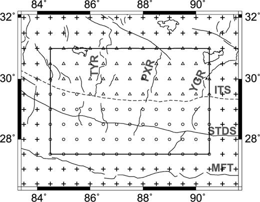
We use the vertical component data from the second phase of the international collaborative Hi-CLIMB project. The second phase of the Hi-CLIMB project consists of two parts: the main N–S trending linear array and the complementary regional array, and records data continuously from 2004 July to 2005 August (Liang et al. 2008; Nabelek et al. 2009). We select a 2-D array out of the whole array (Fig. 1): 33 stations with three types of sensors (Guralp CMG-3ESP, Nanometrics Trillium40, Streckeisen STS-2) from the regional array and five stations with two types of sensors (Guralp CMG-3T, Streckeisen STS-2) from the southernmost part of the linear array. Our array spans ∼500 km in E–W direction and ∼300 km in N–S direction across the ITS. It situates in the blank region between the linear Hi-CLIMB array and the INDEPTH array and its southernmost part overlaps the HIMNT array. The distance between adjacent stations is 25–50 km.

Topographic map of the study region in southern Tibet and broad-band seismic stations selected out of the Hi-CLIMB array. In the main figure, the stations are shown with different symbols representing different types of instruments: Black squares denote stations with the STS-2 sensors, black triangles denote stations with the CMG-3T sensors, black diamonds denote stations with the CMG-3ESP sensors and black circles denote stations with the Trillium-40 sensors. The main tectonic boundaries and the N–S trending rifts are shown as: MFT, Main Frontal Thrust; STDS, Southern Tibet Detachment System; ITS, Indus Tsangpo Suture; TYR, Tangra Yum Co rift; PXY, Pumqu-Xianza rift; YGR, Yadong Gulu rift. In the inset map, the study region is outlined by the open box. The seismic arrays deployed by INDEPTH II, INDEPTH III, HIMNT, Hi-CLIMB are shown with black inverse triangles, blue squares, green triangles and red diamonds, respectively.
2.1 Two-plane-wave Tomography
The seismograms of the earthquakes in a distance range of 33°–120° with MS≥ 5.0 are first cut from the raw data automatically. Because the background noise in Tibet is very low, we are able to obtain 81 events with high-quality seismograms. The backazimuthal distribution of these events is not very good (Fig. 2). Most of them locate on the boundary of the Pacific Plate east of our array. But still some events locate west of our array, which are important for solving for the lateral variations of phase velocities. The ray path coverage is excellent within the array and in the surrounding regions except for the west of the array (Fig. 3).
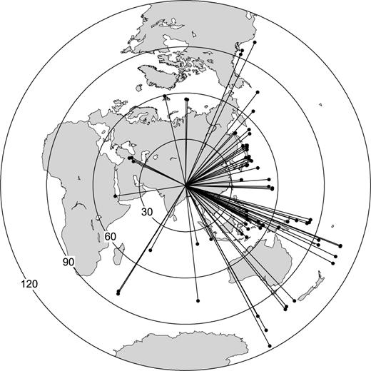
Azimuthal distribution of the teleseismic events used in this study. Epicentral distance from the centre of the seismic array is shown with concentric circles with degrees on the great circle.
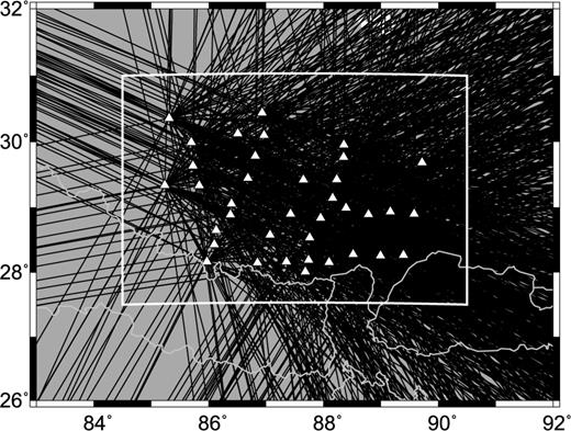
Great circle ray path coverage at the period of 50 s. The study region is marked with the open box. The ray path coverage is excellent within the study region except for the western edge.

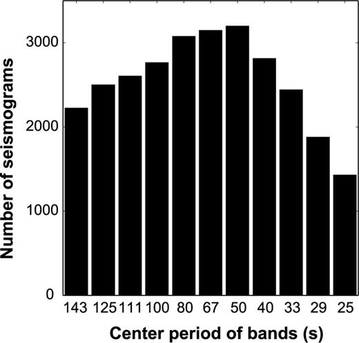
Numbers of the Rayleigh waveforms used at all periods of 25–143 s in the inversions for phase velocities.


2-D Grid of phase velocity model. The study region is marked with the open box. Within the study region, different symbols denote two different tectonic provinces: triangles for the Lhasa block, circles for the Himalayas. Two extra loops of grid nodes (crosses) outside the study region are used to ‘absorb’ some of the phase effects of complex incoming wavefields, which are not properly represented by the interference of two plane waves. The main tectonic boundaries and the N–S trending rifts are marked with the abbreviations as same as in Fig. 1.
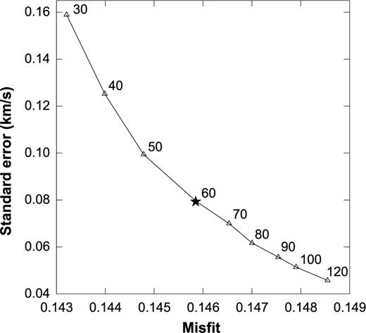
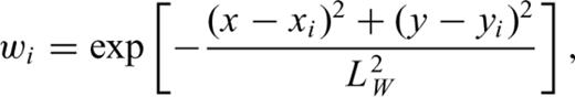
Trade-off curve between model standard errors and misfits of data in the inversions for 2-D isotropic phase velocity model. The trade-off is modified by the characteristic scale length LW (km) in the 2-D Gaussian spatial weighting function (eq. 4). The model standard errors and the misfits of data are the rms of rms through all the frequency bands. The black star marks the selected value for the scale length LW.
For each frequency band, the phase velocities are obtained by iteration. The incoming wavefield of each event is fitted by the interference of two plane waves with different amplitudes, phases and propagating directions. After carefully checking the waveforms mentioned above, the events, whose incoming wavefields are too complex to be fitted by two plane waves, are quite rare. Even if a few of such events are still in the final data set, their influence will be reduced by automatically assigning them small weighing factors in the inversions. According to Forsyth & Li (2005), there are two steps in one iteration. The six wavefield parameters of each event are inverted first by the simulated annealing method. Then a joint inversion for both phase velocities and wavefield parameters is conducted with the generalized non-linear least-squares algorithm (Tarantola & Valette 1982). After one iteration, the priori standard deviations of data in the next iteration are set to the posteriori standard deviations, and the weighting factors are set to the reciprocal of the standard deviations. So the influence of ‘bad’ events is reduced. The iteration repeats towards the final solution. In this study, the priori phase velocity errors are set to 0.2 km s−1 for all nodes inside the study region and 2.0 km s−1 for the two loops of surrounding nodes. The priori standard deviations of data are initially set to 0.1.
2.2 Shear velocity inversion
With the 2-D phase velocity structure as input data, we can establish the 3-D shear wave velocity structure. We invert for 1-D shear wave velocity model at each node in the 2-D phase velocity model and combine the 1-D shear wave velocity models to create a 3-D shear wave velocity model. The inversion procedure adopted in this study was first used by Weeraratne et al. (2003) and Li & Burke (2006). The derivatives of phase velocities with respect to densities and body wave velocities are calculated based on the method of Saito (1988). The invert method is still the generalized non-linear least-squares algorithm (Tarantola & Valette 1982). A layered model is introduced to represent the 1-D shear wave velocity structure. It contains 16 layers from the Earth's surface to the bottom of upper mantle (410 km) including three layers in the crust. Below 410 km, the Earth model maintains the AK135 model (Kennett et al. 1995). Layer thickness is ∼25 km near the Earth's surface and ∼50 km near the bottom of upper mantle. The thickness of the two layers adjacent to the Moho can vary with the Moho depth. Phase velocities of Rayleigh waves are primarily sensitive to shear wave velocities, and insensitive to P-wave velocities deeper than ∼50 km. We keep the densities and Vp/Vs ratios unchanged in the inversions. We use a constant Vp/Vs ratio of 1.72 in the crust derived from the receiver function studies (Jin et al. 2006; Nabelek et al. 2009; Wittlinger et al. 2009). The Vp/Vs ratios in the mantle and the densities follow the AK135 model (Kennett et al. 1995). Therefore, the model parameters in the inversions are reduced to 17 (16 for shear wave velocities and 1 for Moho depth).
As an undetermined inversion problem, the inversions for shear wave velocities can yield a rational solution depending on the proper dumping and smoothing strategy as well as the initial model close to the real. We assign a priori model error of 0.1 km s−1 for dumping the shear wave velocities and a correlation coefficient of 0.4 between adjacent layers for smoothing the model. Particularly, no smoothness is assigned between the top four layers in the model. We have also tried different priori model errors from 0.05 km s−1 to 0.3 km s−1 and selected the proper value to make the resultant model more smooth and vary as much as possible from the initial model. Although the Moho depth is less constrained by Rayleigh-wave phase velocities, we can obtain precise initial Moho depth from receiver function studies. So we assign a small priori model error of 2 km for dumping the Moho depth.
3 Results
3.1 Isotropic phase velocities
We have first inverted for the average phase velocity in the entire study region at each frequency band. The initial average phase velocities are from the dispersion curve of AK135 global model (Kennett et al. 1995). Both the initial AK135 phase velocities and the resultant average phase velocities in southern Tibet are shown in Fig. 7(a). The average phase velocities in southern Tibet are integrally lower than the global averages. Compared with the results in western China (Yao et al. 2005), the average phase velocities in southern Tibet at the periods shorter than ∼70 s are prominently low, but at longer periods the difference of phase velocities is insignificant. Recalling that Rayleigh waves at the periods shorter than ∼70 s mainly sample the crustal structure of Tibet, we suppose that the crustal structure of southern Tibet is a very special case in western China. For example, the average crustal thickness in western China is ∼50 km, while the crustal thickness in southern Tibet is more than 60 km. The abnormally thickened crust in southern Tibet may partly account for the low phase velocities at short periods. The model standard deviations originated from inversion algorithm are fairly small because of only one model parameter in the inversions (Fig. 7).
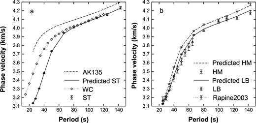
(a) Average Rayleigh-wave phase velocities in Southern Tibet (circles with error bars) compared with those of the global AK135 model (dashed line), and west China (dotted line with open diamonds, Yao et al. 2005). The solid line denotes the predicted dispersion curve in the inversion for 1-D average shear wave velocity model. (b) Average Rayleigh wave phase velocities of two tectonic provinces: the Himalayas (inverted triangles with error bars) and the Lhasa block (circles with error bars). The predicted dispersion curves of the two provinces are plotted with dashed line and solid line, respectively. A comparable result of average phase velocities of the Lhasa block (Rapine et al. 2003) is also plotted with dotted line with diamonds.
We have also inverted for the average phase velocities in the Himalayas and the Lhasa block (Fig. 7b). In the inversions, the nodes in the velocity model were divided into two groups (Fig. 5), and two-phase velocity parameters for two blocks are solved simultaneously. At all periods, the average phase velocities in the Himalayas are ∼0.05 km s−1 higher than those in the Lhasa block, that reflects different lithospheric structures of two blocks in consistent with the previous studies (Cotte et al. 1999; Wittlinger et al. 2004). Rapine et al. (2003) measured the average phase velocities in the Lhasa block using the data recorded by the INDEPTH III array. They measured the phase velocities at the periods shorter than 70 s by the source-station analysis. In Fig. 7(b), our results in the Lhasa block are slightly different from theirs. We think that this slight difference makes sense owing to the very different data sets and analysis approaches. First, our data have better azimuthal coverage than theirs. Second, their study region is much broader than ours. Last, the source-station method they used may cause systemic deviations because the energy of non-planar wavefields is ignored (Wielandt 1993).
With the average phase velocities as initial velocities, we have conducted the inversions for 2-D isotropic phase velocity structure at 11 frequency bands in southern Tibet. Maps of 2-D phase velocity anomalies at the periods of 25, 33, 40, 50, 67, 100, 125 and 143 s are shown in Fig. 8. Velocity anomalies are calculated relative to the average phase velocities in the entire study region. The maps are clipped with the contour of 2 per cent double standard deviations for phase velocity anomalies at the period of 50 s (Fig. 8c). The phase velocities of Rayleigh waves at the periods of 25–50 s are dominantly sensitive to the crustal structure in southern Tibet. Low velocity anomalies mainly appear in the Lhasa block, and are unevenly distributed. The low velocity zones concentrate in the regions of the N–S trending rifts (TYR and PXR). The lateral boundary between high and low velocities extends roughly in E–W direction. At the long periods of 100, 125 and 143 s, the phase velocities mainly reflect the structure of mantle lithosphere. Low velocity anomalies appear beneath the N–S trending rifts and extend southward into the Himalayas. At the same time, the low velocity anomaly beneath the PXR seems to dip eastward. The shape and distribution of phase velocity anomalies at long periods are very different from those at short periods. Particularly, the phase velocity anomalies at 67 s reflect both the lateral velocity variations and the Moho depth undulations. It is hard to extract clear information on the lithosperic structure directly.
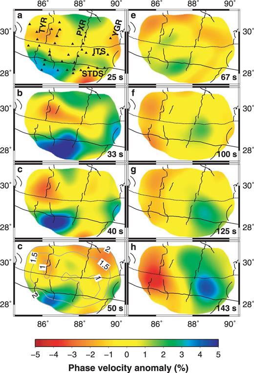
Maps of Rayleigh wave isotropic phase velocity anomalies and standard derivations. The phase velocity anomaly maps are illustrated at the periods of (a) 25 s, (b) 33 s, (c) 40 s, (d) 50 s, (e) 80 s, (f) 100 s, (g) 125 s and (h) 143 s. The velocity anomalies are calculated relative to the average phase velocities in the entire study region. The maps are clipped using the contour of 2 per cent double standard errors at the period of 50 s (Fig. 8d). The black triangles denote the seismic stations (Fig. 8a). The main tectonic boundaries and the N–S trending rifts are marked with the abbreviations as same as in Fig. 1.
We have run a series of checkerboard tests to check the resolution of the resultant 2-D isotropic phase velocity structure. Input velocity anomalies are ±3 per cent relative to the average phase velocities in the entire study region. The synthetic data of amplitudes and phases are calculated based on the ray paths of real data. Gaussian random errors are added to the synthetic data before the inversions. The approach on how to produce the synthetic data and random errors is elaborated in Li et al. (2003). The controlling parameters in the checkerboard inversions are the same as those in the inversions with real data. The results for the checkerboard model with an anomaly size of ∼200 km at short (25 s), intermediate (50 s) and long periods (100 s) are shown in Fig. 9. At all periods, the patterns of velocity anomalies are clearly recovered. The amplitudes of anomalies are recovered at 50 s and partly recovered at 25 and 100 s. We have also run the checkerboard tests with smaller-sized phase velocity anomalies and found that the checkerboard could hardly be recovered at long periods. The reduction of lateral resolution at short and long periods is primarily due to the lack of data coverage (Fig. 4). The improved method with finite frequency kernels is reported to be able to improve the lateral resolution at long periods (Yang & Forsyth 2006).
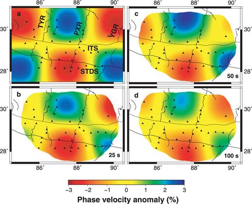
Checkerboard tests for the 2-D isotropic phase velocities. (a) Input model with ±3 per cent anomaly amplitude and 200 km anomaly size. (b–d) Recovered models at short (25 s), intermediate (50 s) and long (100 s) periods. The recovered models are clipped with the same procedure as in Fig. 8(d). The black triangles denote the seismic stations. The main tectonic boundaries and the N–S trending rifts are marked with the abbreviations as same as in Fig. 1.
We have checked the fitting of wavefields in the inversions. The example event occurred at Japan arc on 2004 October 27 with Ms = 5.4. The Rayleigh waves propagated across the heterogeneous continent of Eastern China before arriving to the study region. The observed amplitudes and phases (Figs 10c and d) at 50 s display severe lateral heterogeneity and the energy of non-planar waves is unignorable. As expected, such a complex wavefield is able to be well fitted in the inversions (Figs 10a and c).
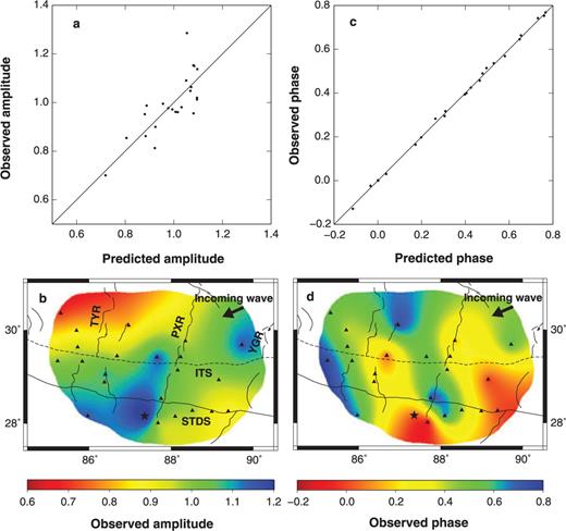
Fitting of the Rayleigh wavefield of the example event at the period of 50 s. The earthquake occurred at Japan arc on 2004 October 27, with Ms = 5.4. (a) and (c) Comparison of predicted and observed normalized amplitudes and phases in the inversion for 2-D isotropic phase velocity model. The amplitudes are normalized by the rms of the observed amplitudes. The phases are calculated relative to the phase at the reference station. (b) and (d) Maps of observed normalized amplitudes and phases. The maps are clipped with the same procedure as in Fig. 8(d). The black arrows denote the incident direction of the Rayleigh waves. 23 stations (triangles and stars) have recorded ‘good’ Rayleigh waveforms. The black stars denote the reference station with zero phases for this event.
3.2 Shear wave velocities
By inverting the average phase velocities, we have obtained the 1-D shear wave velocity models in southern Tibet and two blocks: the Himalayas and the Lhasa block (Fig. 11). The initial model is modified from the AK135 global model (Kennett et al. 1995). The initial Moho depth is 75 km for southern Tibet, 65 km for the Himalayas and 75 km for the Lhasa block according to the receiver function studies (Jin et al. 2006; Nabelek et al. 2009; Wittlinger et al. 2009). To check the dependence on initial models, we have repeated the inversions with different initial models. We find that the main features are consistent among the resultant models. The fitting of phase velocity data is shown in Fig. 7. Compared with the modified AK135 model, the low velocities are observed in the crust of southern Tibet, which is common for the active orogen. But the ultra-low velocity of ∼3.3 km s−1 in the middle crust reflects the existence of partial melting (e.g. Brown et al. 1996; Kind et al. 1996; Nelson et al. 1996; Unsworth et al. 2005). A fast mantle lid is also identified to the depth of ∼160 km with the shear wave velocity of ∼4.7 km s−1, which reflects the underthrusting Indian lithosphere (e.g. Kosarev et al. 1999; Wittlinger et al. 2004). The shear wave velocity in the middle crust of the Himalayas is ∼3.4 km s−1 and ∼3 per cent higher than the Lhasa block. This velocity discrepancy between two blocks is consistent with the previous studies in southern Tibet (e.g. Brown et al. 1996; Kind et al. 1996; Nelson et al. 1996). Decoupled with the Moho depth, the shear wave velocities in the lower crust are approximately equal for the Himalayas and the Lhasa block. The fast mantle lid is imaged to the depth of ∼180 km in the Himalayas and ∼160 km in the Lhasa block. The velocity discrepancy between the Himalayas and the Lhasa block is insignificant in the lower crust and mantle lithosphere. The crustal structure of the Lhasa block in this study is consistent with that from Rapine et al. (2003) except for the structure nearby the Moho. This difference is caused by the different settings in the inversions: We set a priori Moho in the velocity model, but they did not.
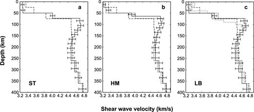
1-D average shear wave velocities in (a) southern Tibet and two tectonic provinces: (b) the Himalayas and (c) the Lhasa block. The resultant shear wave velocities are plotted with solid lines with error bars. The modified AK135 global model with the crustal thickness of 75 km (Kennett et al. 1995) is plotted with dashed lines. The average shear wave velocities in southern Tibet are plotted with grey solid lines in Fig. 11(b) and (c) for comparison. Another shear wave velocity model in the Lhasa block (Rapine et al. 2003) is shown with dotted line in Fig. 11(c).
Rayleigh-wave phase velocities at different periods are primarily sensitive to shear wave velocities at different depths. As shown in Fig. 12(a), the sensitivity kernel at the shortest period (25 s) reaches the peak value at the depth of ∼25 km and at the longest period (143 s) reaches the peak value at the depth of ∼200 km. So the resultant shear wave velocity models have good depth resolution at the depths of 25–200 km. On the other hand, the sensitivity kernels at long periods become much flatter and have smaller peak values than at short periods. As a result, the resolution to shear wave velocities decreases with depth. We confirm the decreasing of resolution with depth in the model resolution matrix (Fig. 12b). The resolution to shear wave velocities at each layer peaks at the right depth, but their peak values become smaller as the depths of layers increase. There are total five pieces of independent information derived from the 1-D inversion: ∼0.85 for shear wave velocity at the depths of 25–50 km, ∼0.7 at the depths of 50–73 km (the Moho) and ∼1.6 at the depths of 73–200 km. So the average velocities in the middle crust, lower crust and mantle lithosphere can be well determined.
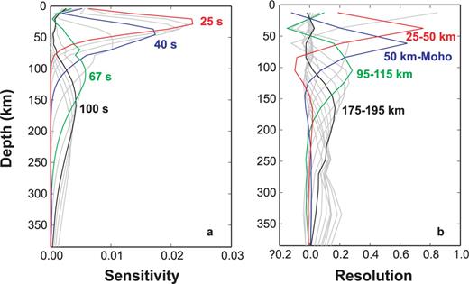
(a) Rayleigh wave phase velocity sensitivity kernels to the 1-D average shear wave velocity model in southern Tibet. The kernel at the shortest period (25 s) has a peak sensitivity of ∼25 km and at the longest period (143 s) has a peak sensitivity of ∼200 km. (b) Rows of the resolution matrix for the average shear wave velocity model in southern Tibet. The resolution for each layer corresponds to one row of the matrix and is plotted with a curve. The sharper the peak is, the higher the resolution is for that layer.
With the same inversion procedure, we have inverted for 1-D shear wave velocity models at each node in the 2-D phase velocity model to obtain a 3-D model in southern Tibet. The lithosphere structure observed directly from phase velocities is vague and even misleading without correction for the crustal thickness (e.g. Griot et al. 1998). The joint inversion of shear wave velocities and crustal thickness can solve the problem, but bring in the trade-off between them. We change the initial model to the more realistic 1-D average shear wave velocity model in southern Tibet and interpolate the crustal thickness derived from the receiver function studies using the Hi-CLIMB data (Jin et al. 2006; Nabelek et al. 2009) to obtain the initial map of crustal thickness. The crustal thickness is more heavily damped than shear wave velocities in the inversions because the initial crustal thickness is fairly accurate. The resolution of the resultant 3-D shear wave velocity model can be derived from both the lateral resolution of 2-D phase velocity inversions and the depth resolution of 1-D shear wave velocity inversions.
The resultant 3-D shear velocity model of the crust is shown in Fig. 13. The shape and distribution of shear wave velocity anomalies are remarkably different between the middle and lower crust, which reflects the existence of a decollement between the middle and lower crust (Burchfiel et al. 1989; Zhao et al. 1993; Hauck et al. 1998). This decollement was widely observed in southern Tibet by the previous studies (Brown et al. 1996; Nelson et al. 1996; Schulte-Pelkum et al. 2005; Nabelek et al. 2009). In the middle crust, a large low velocity anomaly appears in the Lhasa block. Such a low velocity anomaly was also imaged by INDEPTH data and interpreted as the presence of partial melting (Brown et al. 1996; Makovsky . 1996; Nelson et al. 1996; Unsworth et al. 2005). In the lower crust, low velocity anomalies appear along the TYR and PXR.
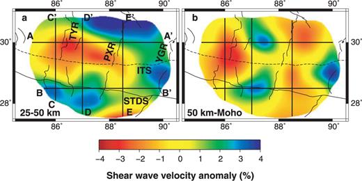
Maps of shear wave velocity anomalies in the crust: (a) 25–50 km and (b) 50 km–Moho. The velocity anomalies are calculated relative to the average shear wave velocity in southern Tibet. The maps are clipped with the same procedure as in Fig. 8(d). The main tectonic boundaries and the N–S trending rifts are marked with the abbreviations as same as in Fig. 1. Locations of vertical profiles are plotted either.
The resultant 3-D shear wave velocity model of the mantle lithosphere is shown in Fig. 14. The low velocity anomalies continue appearing along the N–S trending rifts in consistent with the velocity structure in the lower crust. The low velocity anomalies along the TYR and PXR can be recognized from the lower crust to the bottom of lithosphere. The similar low velocity anomalies were imaged along the N–S trending rifts in southern and southeastern Tibet (Ren & Shen 2008; Hung et al. 2010; Liang et al. 2011). The low velocity structure beneath the PXR seems to dip eastward. High velocity anomalies appear in the non-rift regions, which is consistent with the obvious interpretation that the Indian lithosphere is underthrusting beneath southern Tibet.

Maps of shear wave velocity anomalies in the mantle: (a) Moho–95km, (b) 95–115 km, (c) 115–135 km, (d) 135–155 km, (e) 155–175 km and (f) 175–195 km. The velocity anomalies are calculated relative to the average shear wave velocity in southern Tibet. The maps are clipped with the same procedure as in Fig. 8(d). The main tectonic boundaries and the N–S trending rifts are marked with the abbreviations as same as in Fig. 1. Locations of vertical profiles are plotted either.
Four vertical profiles are presented in Fig. 15 to highlight the differences among these rifts and between rifts and non-rift regions. The profiles A–A′ and B–B′ situate in the Lhasa block and the Himalayas, respectively. They extend across the TYR and PXR from west to east. The profiles C–C′ and E–E′ run along the TYR and PXR, respectively and the profile D–D′ is in the non-rift regions between them. The E–W trending profiles (A–A′ and B–B′) show prominent low velocity anomalies along the TYR and PXR from the lower crust to mantle lithosphere. The lower boundary of the low velocity anomaly along the TYR is beyond 200 km deep, while the low velocity anomaly along the PXR terminates at the depth of ∼150 km or dips eastward. We cannot make a conclusion which state is real because of the lateral smearing at that depth. The N–S trending profiles (C–C′, D–D′ and E–E′) show a clear structural contrast between rifts and non-rift regions. The low velocity anomalies beneath the rifts are uninterrupted from the lower crust to the mantle lithosphere and from the Himalayas to the Lhasa block. A slab-like high velocity anomaly is observed across southern Tibet beneath the non-rift regions.
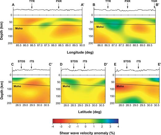
Vertical profiles of shear wave velocity anomalies. Profiles A–A′ and B–B′ are along latitude 30°N and 28.5°N. Profiles C–C′, D–D′ and E–E′ are along longitude 86°E, 87°E and 88.5°E. Locations of these profiles are shown in Figs 13 and 14. The velocity anomalies are calculated relative to the average shear wave velocity in southern Tibet. Topography and Moho are plotted above and in the velocity anomaly profiles. The main geological boundaries and the N–S trending rifts are marked with the abbreviations as same as in Fig. 1.
4 Discussions
4.1 Crustal Channel flow in southern Tibet
Observations of coincident low seismic velocity anomalies (Kind et al. 1996; Nelson et al. 1996; Hung et al. 2010), low electric resistivity (Pham et al. 1986; Chen et al. 1996; Wei et al. 2001; Unsworth et al. 2005), reflection bright spots (Brown et al. 1996; Makovsky et al. 1996) and high heat flow (Francheteau et al. 1984) in southern Tibet all attest to the presence of partial melt and/or aqueous fluids in the middle and/or lower crust. These observations are commonly interpreted as strong evidences for southward crustal channel flow (Beaumont et al. 2001, 2004; Unsworth et al. 2005). The notion of crustal channel flow is very popular to explain the E–W extension of central and eastern Tibet (e.g. Clark & Royden 2000; Royden et al. 2008). But whether the channel flow exists in southern Tibet or not and how it distributes are controversial (Chung et al. 2005; Hung et al. 2010).
Our results show a pervasive low shear wave velocity anomaly in the middle crust of the Lhasa block (Fig. 13a), which covers the N–S trending rifts and non-rift regions. But the low velocity anomalies along the rifts in the lower crust are not interconnected (Fig. 13b), which is consistent with the observation of Hung et al. (2010). The very different structures in the middle and lower crust are not artificial because they can also be recognized from the 2-D phase velocity anomaly models (Fig. 8). The INDEPTH geophysical investigations (e.g. Nelson et al. 1996; Unsworth et al. 2005) suggested a wholesale channel flow model in the middle crust. But both their seismic and magnetotelluric profiles are along the N–S trending rifts and provide no constrains on the structure of non-rift regions. Hung et al. (2010) argued that the wholesale crustal channel flow model is untenable because their 3-D body wave tomography results indicated that the low velocity anomalies in the lower crust concentrated beneath the rifts and were not interconnected. Our results reconcile the wholesale crustal channel flow model proposed by the INDEPTH projects and the 3-D tomography results of Hung et al. (2010), and support the pervasive mid-crustal channel flow in southern Tibet.
Seismic tomography can only provide constrains on the current status of the lithosphere in southern Tibet. The observed low velocity anomaly in the middle crust does not corroborate the presence of Miocene channel flow in the middle crust. The emplacement of Himalayan leucogranites, and rapid exhumation and metamorphism along the southernmost Tethyan Himalayas are usually attributed to the Miocene crustal channel flow (Zeitler et al. 2001; Beaumont et al. 2004). But studies on the Miocene magmatism in the Lhasa block indicated the widespread occurrence of ultrapotassic and adakitic magmatism, which were interpreted as melts of the metasomatized lithospheric mantle and mafic lower crust, respectively (Williams et al. 2001; Chung et al. 2005). If it existed, the Miocene channel flow would be likely to occur in the lower crust and be very different from the current channel flow in the middle crust.
4.2 N–S trending rifts in southern Tibet
The geological history of the salient N–S trending rifts in southern Tibet, which relate to Cenozoic E–W extension of the plateau, has been a puzzle for more than three decades (Taylor & Yin 2009). Previous studies tended to the explanation that the rifts in southern Tibet were restricted only to the upper crust, based on the analysis of rift flank topography (Masek et al. 1994) and geophysical observations (Cogan et al. 1998; Nelson et al. 1996). To the contrary, Instability analysis based on rift spacing requires a coherent E–W extension throughout the entire crust and mantle lithosphere (Yin 2000). Focal depths and mechanisms of the earthquakes directly beneath the rifts further suggest the brittle E–W extension are accommodated by both the upper crust and the upper mantle (Chen & Molnar 1983; Zhu & Helmberger 1996; Chen & Yang 2004). Furthermore, recent body wave tomography studies provided direct contrary evidences, that low velocity anomalies from the lower crust to the mantle lithosphere were imaged along the rifts (Ren & Shen 2008; Hung et al. 2010; Liang et al. 2011). The conflict observations also occur in our results. Both the pervasive low velocity anomaly in the middle crust and the difference of the shape and distribution of velocity anomalies between the middle and lower crust reflect the presence of structure decoupling in the crust of southern Tibet (Fig. 13). This decoupling leads to the conclusion that the N–S trending rifts are restricted in the upper crust. While the low velocity anomalies from the lower crust to the mantle lithosphere along the TYR and the PXR argue that the formation of these rifts is associated with the entire lithosphere (Figs 13–15). The paradoxical implications on the N–S trending rifts reflect that the formation of the rifts is a complicated multistage tectonic process, which is supported by the recent geological investigation (Kapp et al. 2008).
Comparison of igneous activity and age of onset of rifting in southern Tibet may provide some insights on this multistage tectonic process. Geochemical and geochronological studies on the igneous rocks in southern Tibet suggested the Miocene ultrapotassic and adakitic magmatism (∼26 to 10 Ma) was nearly coeval with onset of the E–W extension (Williams et al. 2004; Chung et al. 2005). They also found that the magma dyke swarms were often associated with the N–S trending rifts (Williams et al. 2001). Local asthenospheric upwelling is implied from the presence of ultrapotassic and adakitic magmas along the rifts, which originate from the mantle lithosphere and the lower crust, and leads to the break of the entire lithosphere along the rifts in southern Tibet at ∼26–10 Ma. The starting age of the N–S trending rifts in southern Tibet is usually constrained to be later than ∼8 Ma (Harrison et al. 1995; Yin et al. 1999; Maheo et al. 2007). The age discrepancy between the onset of rifting and the Miocene magmatism denies the simple model that the N–S trending rifts are formed though a coherent deformation throughout the entire lithosphere. We present a possible scenario as follows: In the early stage (∼26–10 Ma), the Miocene magmatism broke the entire lithosphere along the N–S trending rifts. The rifts initiated with the coherent rifting throughout the entire lithosphere. In the late stage (after ∼8 Ma), the occurrence of partial melting in the middle crust destroyed the coherent rifting throughout the lithosphere. The rifting continued and was restricted in the upper crust. The current N–S trending rifts in southern Tibet are decoupled with the lower crust and mantle lithosphere because of the wholesale mid-crustal channel flow derived from this study as well as the previous studies (e.g. Nelson et al. 1996; Unsworth et al. 2005). The geological history of these rifts is yet close associated with the deformation or break of the entire lithosphere.
4.3 The Indian lithosphere beneath the Tibet
There is no doubt that the shape of the Indian lithosphere beneath the Tibet plays a key role in the tectonic evolution of the plateau. Recent studies using the data acquired from the Hi-CLIMB array indicated that the subhorizontally underthrusting Indian mantle lithosphere reached ∼100 km north of the BNS (∼33°N, Chen et al. 2010; Hung et al. 2010) and the underthrusing Indian lower crust slid to ∼31°N (Nabelek et al. 2009). Furthermore, the underthrusting of the Indian lithosphere is along distributed evolving subparallel structures (Nabelek et al. 2009; Liang et al. 2011). Our results show no constrains on these interior boundaries because of the limitation of the study region and the inherence of surface waves. But the presence of a slab-like high velocity anomaly in the non-rift regions (Fig. 15), which can be traced from the Himalayas to the Lhasa block, is consistent with the implication of a subhorizontally underthrusting Indian lithosphere. On the other hand, the presence of low velocity anomalies from the lower crust to the mantle lithosphere along the N–S trending rifts in this study as well as in the recent studies (Ren & Shen 2008; Hung et al. 2010; Liang et al. 2011) suggests that the underthrusting Indian lithosphere has been broken into pieces during the E–W extension of the plateau. As a corollary, we conclude that the central part (∼85°E–90°E) of southern Tibet is now underlain by the broken Indian lower crust and mantle lithosphere.
5 Conclusions
We have carried out the Rayleigh-wave tomography in southern Tibet with the data recorded by a 2-D seismic array, which is a part of the Hi-CLIMB array. A 3-D shear wave velocity model is established for the lithosphere structure in southern Tibet.
A pervasive low shear wave velocity anomaly is observed in the middle crust of the Lhasa block, which supports the wholesale mid-crustal channel flow in southern Tibet. Previous evidences for the mid-crustal channel flow were derived from the seismic and magnetotelluric profiles along the N–S trending rifts (e.g. Nelson et al. 1996; Unsworth et al. 2005). Our results confirm the presence of low velocity anomalies in the middle crust of non-rift regions. In the lower crust, low shear wave velocity anomalies are observed along the TYR and PXR. The shape and distribution of velocity anomalies are remarkably different between the middle and lower crust, which reflects the structural decoupling between the middle and lower crust.
The low shear wave velocity anomalies along the TYR and PXR are imaged from the lower crust to the bottom of lithosphere and from the Himalayas to the Lhasa block. The lower boundary of the low velocity anomaly beneath the TYR is beyond 200 km deep, while the low velocity anomaly beneath the PXR terminates at the depth of ∼150 km or dips eastward. A simple rifting model cannot interpret the current coexistence of (1) the structural decoupling between the middle and lower crust and (2) the low velocity anomalies from the lower crust to the mantle lithosphere beneath the N–S trending rifts. We propose that the rifting along the N–S trending rifts is a coherent deformation throughout the entire lithosphere in the early stage and then decoupled with the lower crust and mantle lithosphere in the late stage. The current N–S trending rifts in southern Tibet are restricted in the upper crust.
In the non-rift regions, a slab-like high velocity anomaly is identified beneath both the Himalayas and the Lhasa block, which is interpreted as the underthrusting Indian lithosphere. Together with the observations of low velocity anomalies along the TYR and PXR, we suggest the central part of southern Tibet is now underlain by the broken Indian lower crust and mantle lithosphere.
Acknowledgments
We thank John Nabelek and his HI-CLIMB field team for their hard work at the southern Tibet to collect the data used in this study. We thank Eric Sandvol and Yingjie Yang for applying the tomography codes. We also thank three anonymous reviewers for their constructive comments, which improve the manuscript. All figures in this paper were plotted with the Generic Mapping Tools (Wessel, P. & Smith, W.H.F.). This study is funded by Natural science fundation of China (grant number: 40774017 and 40904022). Mingming Jiang acknowledges China Scholarship Council supported the study trip to United States.
Supporting Information
Additional Supporting Information may be found in the online version of this article:
Supplement. The inversion for shear wave velocities is an underdetermined inversion problem. The dumping and smoothing strategy and the initial model should be determined carefully. We have tried different priori standard deviations of 0.05, 0.1, 0.15, 0.2, 0.25 and 0.3 km s−1 for shear wave velocities to find the proper dumping. The results are shown in Fig. S1. The difference of the mantle structure caused by different dumping parameters is insignificant compared with that of the crustal structure.We select a proper value of 0.1 km −1 because the resultant model is smooth and deviates as much as possible from the initial model. We also conducted a random experiment to check the dependence on the initial model. We disturbed the shear wave velocities in all layers of initial model with random noises and ran the inversions with disturbed initial models 1000 times. The random noises are drawn from the uniform distribution on the interval (−0.1 km −1, 0.1 km −1). The results are shown in Fig. S2. We find that the main features of the optimum model are unchanged despite disturbed initial models. Their effects on the optimum model are trivial.
Please note: Wiley-Blackwell are not responsible for the content or functionality of any supporting materials supplied by the authors. Any queries (other than missing material) should be directed to the corresponding author for the article.
References
