An EGF-based methodology for predicting compatible seismograms in the spectral domain using GA technique

Summary

1 Introduction

In regions with a lack of sufficient reliable, such as the region under study, synthesizing spectrum compatible strong motions, consistent with regional source mechanism, path and site soil condition are very useful in engineering purposes. The reliability of synthesized seismograms depends strongly upon a reasonable model being developed, consistency with the faulting process of the event and estimation of appropriate model parameters such as; focal mechanism (strike, dip and rake), rise-time, rupture velocity, hypocentre location, wave path propagation effects and site soil conditions.

Over the last decade, various methods for estimating ground shaking can be found in the literature. Aki (1968) and Haskell (1969) were the first researchers who successfully investigated a theoretically based estimation of strong motions using kinematic source model for propagating dislocation over a fault plane in an infinite homogeneous medium. The point source model proposed by Brune (1970) produces ground shaking on the basis of an ω-squared source spectra. However, it appeared to be unable to describe long duration of large earthquakes and also near-field problems such as directivity and fling step.

The dynamic rupture process on the fault and the heterogeneous structures around the source and observation sites, which are extremely cumbersome, were effectively investigated by Hartzell (1978). He proposed an approach, known as ‘Empirical Green's function (EGF) method’ for synthesizing broad-band seismograms using observed records from small events occurring around the source area of a large earthquake. Subsequently, Irikura & Muramatu (1982), Imagawa & Mikumo (1982) and Iida & Hakuno (1982) attempted to synthesize the mainshock motions using small shock motions such as foreshocks and aftershocks. The method was used and developed by Mueller (1985), Mori & Frankel (1990) and Hutchings (1991). The most important merit of the EGF approach is that, the effects of path from source up to beneath the site and surface soil condition are taken into account (Lam et al. 2000). The basic assumption in this method is that both strong and weak earthquakes have similar focal mechanisms and are located close to each other, but this is not always true. The EGF method can be applied both in inverse and direct problems. In the former, EGF helps to retrieve the focal mechanism and the source time function (Mueller 1985; Frankel et al. 1986; Mori & Frankel 1990; Plicka 2003). This paper is not attempting to derive the specific rupture model, but rather a model that can be effectively used to simulate compatible seismograms for engineering purposes. The approach proposed by Hutchings & Wu (1990) is adopted for simulating seismogram and predicting waveform at the sites, in the region under study, where EGF is not recorded. The basic theory of the proposed approach is that, the record of a weak event, with its hypocentre matching the ordinates of an element on the assumed rupture surface, is assigned as EGF to this element. For elements, which are not matched by EGFs, the closest earthquakes are extrapolated by correcting radiation pattern, attenuation and traveltimes (Hutchings 1991). When EGFs are not obtained for all possible elemental source locations, we approximate the EGF, in frequency domain, proposed by Hutchings & Wu (1990) as

1

where, X is hypocentral distance, B is the radiation coefficient. Subscripts i and o refer to values for the elemental source and the source event, respectively. Q is used to correct for attenuation due to differences in whole-path propagation distance. Q values near the source and recording site are not corrected and are assumed to be captured in the EGF recording. c is the seismic velocity over the travel path. Corrections are applied separately to the P- and S-wave portions of the seismogram. More information is available from Hutchings (1991). We adopted EGFs, as defined by Hutchings & Wu (1990), to be recordings of effectively impulsive point sources, that is, rise time, rupture duration or source dimensions are small enough that their effect cannot be observed in the frequency band of interest. In addition, stress drop changes are reflected in the differences of their seismic moment. We deconvolved out their finite Brune source to effectively create impulsive point source events (Hutchings et al. 2007). Slip at an element follows a ramp function that has amplitude determined by the Kostrov slip function (Burridge & Willis 1969). For each element a slip function, resulting from Kostrov slip model (Hutchings 1991) is convolved with its EGF and multiplied by element moment to calculate the slip function. A summation of step functions is used to model the Kostrov slip function in time domain. The time delay for the step function's summation is at the digital-sampling rate of the EGFs to ensure that high-frequency artefacts are higher than the frequency range of interest. Hutchings (1994) shows that the difference in computed seismograms using the ramp to model the shape of the Kostrov slip function was in the frequency range of 0.5 to at least 15.0 Hz (Hutchings et al. 1997). The question, ‘how is the high frequency in the syntheses produced?’, is comprehensively discussed in (Hutchings 1994). Finally, the records are summed in the order of the rupture front that propagates with an assumed rupture velocity starting at the hypocentre. In this paper, the soil response is assumed to be linear and the soil non-linearity is not taken into account even though the soil might respond non-linearly.

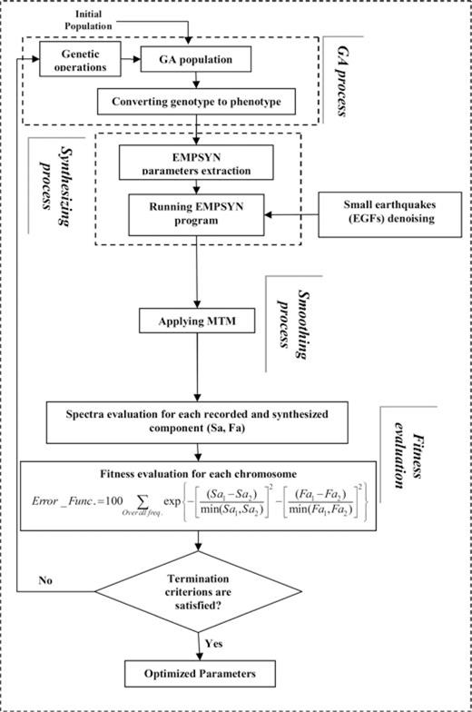
This paper starts with a brief explanation on the scopes and objectives and the problems faced through this study. Aftershock denoising and the MultiTaper Method (MTM) are briefly discussed and the results from the two approaches employed are verified in the next sections. The subsequent sections are devoted to a description of the Genetic Algorithm (GA) technique development and explanation of simulating waveform methods particularly the EGF approach, the MTM and verification and minimization of spectral leakage. The next sections are devoted to a case study of the 2006 Silakhor earthquake seismicity and source data model validation, results, comparison of the results with those of other investigators. Comparison of the obtained response spectrum, Fourier spectra and time histories are discussed in the next section. Finally, this paper ends with a summary and conclusions.

2 Objectives and Scopes

Seismic codes of practice such as Federal Emergency Management Agency (1997) (Chapter 2.6), American Society of Civil Engineers –(2005) (chapter 21, p. 206) and Federal Emergency Management Agency (2000) (chapter 1.6) state that, the performance evaluation of existing and/or new structures is permitted to be done using elastic ‘response spectra with 5 per cent damping ratio’, or ‘specific site response spectrum’. In addition, American Society of Civil Engineers (2010) (16.13.2, 3-D Analysis), states that, ‘Where the required number of recorded ground motion pairs is not available, appropriate simulated ground motion pairs are permitted to be used to make up the total number required’.

This paper is intended to present a methodology for realistic prediction of spectrum compatible seismograms at sites where main shock is not recorded from sites at which the main event has been observed using the EGF approach. The proposed methodology is efficiently useful for producing spectrum realistic compatible seismograms in the form of three components L, T and V. These waveforms make up the total number of requirement for dynamic linear and non-linear analysis of structures in regions with lack of a sufficient data such as that under study. For this purpose, an EGF-based approach is employed for calibration and synthesizing far field acceleration time history. However, the technique is claimed to be applicable to near source sites (Scognamiglio & Hutchings 2009).

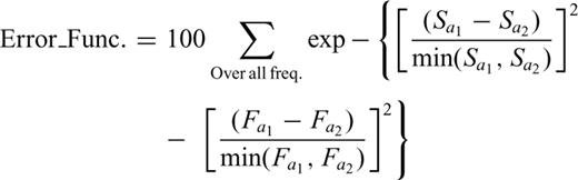
Due to the fact that the Silakhor aftershock records suffer from urban seismic noise (USN), which will be discussed later, we tried to denoise the aftershocks with a high signal-to-noise ratio (SNR < 3). To produce spectrum compatible synthetic seismograms, the well-known MultiTaper Spectrum (MTS) technique developed by Park et al. (1987b) is employed to reduce the spectral leakage. A GA technique (Nicknam & Eslamian 2010) is used for performing the inversion solution problem aimed at minimizing the errors between the response spectra and Fourier spectral amplitudes corresponding to the synthesized and observed seismograms. Among scoring 10 quantitative seismogram characteristics measure criteria recommended by Anderson (2004), we paid special attention to elastic response and Fourier amplitude spectra corresponding to the synthetic and observed seismograms. However, this technique permits minimizing the errors due to more earthquake quantitative measure criteria such as Arias intensity, peak ground acceleration and peak ground velocity. Nevertheless, based on the experience of the authors, the converging process time cost depends strongly upon the number of earthquake characteristic criteria being involved. The proposed technique is implemented to the 2006 Silakhor earthquake (M_w= 6.1) as an example. These issues are discussed in subsequent sections.

3 Urban Seismic Noise Sources (USN)

In general, the measurements made in geophysical exploration, particularly in small events such as aftershocks, are contaminated by unavoidable noises. These noises are evaluated by a SNR, the ratio of the signal and noise spectra. Data acquired in urban areas are often strongly affected by noise (Parolai 2009). The USN can be considered as mainly caused by human activity for example, cars, factories ‘microtremor’ for higher frequency (>1 Hz, 1–0.1 s) that attenuates within several kilometres in distance and depth and those mostly dominated by natural sources ‘microseism’ for lower frequency (<0.6 Hz; Bonnefoy-Claudet et al. 2006). In the frequency range of 0.6–1 Hz both man-made and natural sources might overlap and cause powerful noise (Groos & Ritter 2009). Low SNRs may become an inhibiting factor when trying to estimate ground motion and site response and its effects on large structures with natural frequencies below 0.5 Hz (Rodgers et al. 2003).

4 Aftershock Denoising

Donoho & Johnstone (1995) pioneered the work on filtering of additive Gaussian noise using wavelet thresholding. The term wavelet thresholding is explained as decomposition of the data into wavelet coefficients, comparing the detail coefficients with a given threshold value and shrinking these coefficients close to zero to take away the effect of noise in the data. The time history is reconstructed from the modified coefficients. During thresholding, a wavelet coefficient is compared with a given threshold and is set to zero if its magnitude is less than the threshold; otherwise, it is retained or modified depending on the threshold rule. Thresholding distinguishes between the coefficients due to noise and the ones consisting of important signal information. There exist various methods for wavelet thresholding, which rely on the choice of a threshold value. The two general categories of thresholding are hard and soft-thresholding types. In hard-thresholding T_H can be defined as (Donoho 1995)

2

Here t is the threshold value. Thus, all coefficients whose magnitude is greater than the selected threshold value t, remain as they are and the others with magnitudes smaller than t are set to zero. It creates a region around zero where the coefficients are considered negligible. Soft-thresholding is where coefficients greater than the threshold are shrunk towards zero after comparing them to a threshold value. It is defined as follows (Donoho 1995)

3

Here t is the threshold value. A plot of T_H (left-hand side) and T_S (right-hand side) are shown in Fig. 1.

Figure 1

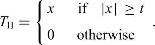
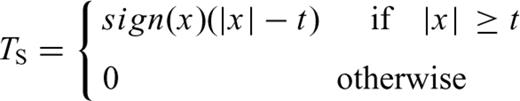
Definition of the T_H for hard-thresholding (left-hand side) and the T_S for soft-thresholding (right-hand side).

Open in new tabDownload slide

In practice application of wavelet-based soft method is preferred (Ansari et al. 2010). Therefore we employed this method, which yields more visually pleasant results with a smaller minimum mean squared error compared to the hard form of thresholding (Donoho 1995). For this purpose, a computer program was developed using MATLAB code by which aftershock denoising processes were carried out. It is worth noting that, the paper is not intended to characterize the frequency-dependent noise levels of aftershocks. Useful frequency range has been defined for each signal as where the SNR is greater than 3 over a continuous bandwidth (e.g. >10 Hz or <0.6 Hz; Parolai 2009; Edwards et al. 2010). We used trial and error approach for reducing frequency-dependent seismic noise associated with aftershocks by increasing the SNR level up to 3. This SNR level was different for each signal. Fig. 2 shows a typical frequency-dependent noisy and denoised aftershock using in the EGF method. In this figure, the Fourier spectral amplitude and the elastic response spectra, corresponding to a small earthquake EGF, and that of denoised signal are compared. As is seen, at low frequency an ω²slope for the acceleration spectrum down to 0.4 Hz is seen (Brune 1970). Below 0.4 Hz the noises can be observed from instrumental, microseism, computational, etc. (e.g. Groos & Ritter 2009).

Figure 2

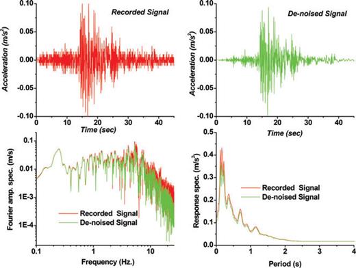
Schematic demonstration of a noisy and denoised small earthquake, Fourier spectral amplitudes and corresponding response spectra. As is seen, at low frequency an ω² slope for the acceleration spectrum down to 0.4 Hz is visible (Brune 1970). Below 0.4 Hz the noises from instrumental, microseism, computational, etc. is observed (e.g. Groos & Ritter 2009).

Open in new tabDownload slide

5 MTM Used, Verification and Minimization of Spectral Leakage

Seismic signals have very high dynamic range, which might lead to severely biased estimates due to spectral leakage, where frequency information with high amplitudes leaks into frequency regions with low amplitudes (Prieto 2007). The MTS algorithm introduced by Thomson (1982, 1990) has been widely used in the geophysical community (e.g. Park et al. 1987a,b; Park 1992; Prieto et al. 2007a, b). The method takes advantage of a family of orthogonal tapers, which are resistant to spectral leakage. The estimated MTS is strongly influenced by the choice of the taper that is easily observable by expressing eq. (4) as a convolution of the taper transform and the true spectrum.

4

where F_N is nyquist frequency . According to eq. (4), a good taper will have a spectral window with low amplitudes whenever | f − f′ | is large. The ordered eigenvalues 1 ≻λ₀≻λ₁≻λ₂≻ ... and associated eigenvectors V^(k) (N, W); k = 0, 1, 2, 3…N–1, so-called prolate eigentapers (Slepian 1978), which have components V^(k) ; t = 0, 1, 2, 3… , are used to suppress the spectral leakages. The prolate eigentaper with a time bandwidth of P = NW, so-called the p π prolate taper, concentrates spectral energy in a time bandwidth product of 2w = 2P/N and minimizes the spectral leakages at frequency ffrom outside the frequency band defined by . To minimize spectral leakage we did plenty tests and finally found the 4 π prolate eigentapers associated with nine eigenvectors, k, yield the best values. More details about MTM are available in Prieto et al. (2007a, b).

We employed the MTM library written by Prieto et al. (2007a,b, 2009), in FORTRAN 90 language for estimating the MTS corresponding to the synthesized and observed waveforms. The technique produces millions of time-series for finding those associated with the minimum error. This efficiency of the MTM being used was verified through applying the 2003 Bam earthquake (Nicknam & Eslamian 2010). Fig. 3 shows the recorded acceleration time history, the Fourier spectral amplitudes and elastic response spectrum with 5 per cent damping ratio corresponding to the original signal (blue coloured). The efficiency of MTM used is quite visible in the figure. The figure also illustrates comparison of the inverse signal into time domain together with the corresponding response spectrum (Red coloured). A good match of the two response spectra confirms the efficiency, validity of the MTM and inversing process being used (see right-hand side figure, red coloured). To demonstrate the efficiency of the nine eigenvectors used in MTM, we used a cosine taper and followed the problem through a signal-tapered procedure. Fig. 3 demonstrates the efficiency of using nine prolate-tapers compared with that of single taper.

Figure 3

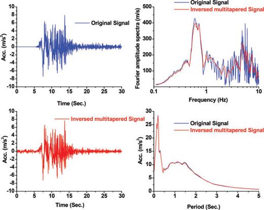
Comparison illustration of Fourier spectral amplitude and elastic response spectra corresponding to the original signal (blue coloured) and inversed MTS (red coloured). The result of single cosine-tapered is also shown.

Open in new tabDownload slide

6 Genetic Algorithm

One of the methods in inversion problems aimed at minimizing the differences between synthesized seismogram and that of the observed data is the GA technique. This technique, as an optimization procedure, has also been successfully applied to structural design (Camp et al. 1998). Jimenez et al. (2005) applied the GA method in an inversion approach to find earthquake source parameters and attenuation factors. Wu et al. (2008) used the GA approach to find focal mechanism in Taiwan. More details of GA can be found in (Haupt & Haupt 2004).

We applied the GA technique for minimizing the differences between Fourier spectral amplitudes and response spectra (5 per cent damping ratio) corresponding to the three components of simulated seismograms and recorded data.

The mathematical expressions for evaluating the fitness function for the GA of individuals in a generation are as follows

5

The mathematic form of evaluating goodness of fit, proposed by Anderson (2004), in shown in the form

6

where the fitness parameter S(P₁, P₂), stands for any type of earthquake characteristic. The two fitness parameters S(S_a1, S_a2) and S(F_a1− F_a2) are used in this study where S_a1, S_a2 and F_a1, F_a2 are response spectral amplitudes and Fourier spectral amplitudes corresponding to the synthetic and observed data at each period and frequency, respectively. More details are found in the Anderson (2004). The mathematic error function is calculated by summing the two parameters S(S_a1, S_a2) and S(F_a1− F_a2),over the whole periods and frequencies of the synthetic and corresponding observed earthquake components (L, T and V), using eq. 7 (Cases 6 and 8, Table 1, Anderson 2004).

7

The main steps of the proposed GA technique are shown in the flowchart of Fig. 4.

Table 1

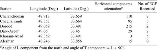
Station names, locations and number of recorded EGFs during Silakhor earthquake.

Open in new tabDownload slide

Figure 4

Proposed GA model.

Open in new tabDownload slide

7 Synthesizing Waveform Method

Following Frankel et al. (1995), the ground acceleration at the station during the main event can be expressed as a sum of N convolutions to obtain the following equation

8

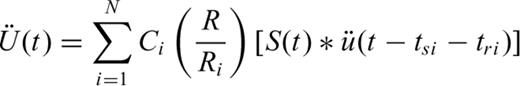
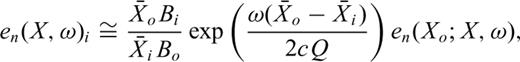
Where is the recorded acceleration (EGF) corresponding to subfault i. C_i is the ratio of the stress drop in the ith subfault to that of the small aftershock event. R_i is the distance of the ith fault to the surface station and R is the hypocentral distance between the station and the source of the aftershock. The shear-wave traveltime t_si from ith fault to the station can be computed from the velocity model. We adopted the method proposed by Hutchings et al. (2007) for estimating synthetic seismograms by numerically computing the discredited representation relation with EGF. The formula it uses has the following form (Hutchings et al. 2007)

9

where X and t are position in space and time relative to the hypocentre and the origin time of the synthesized earthquake, respectively. N is the number of elements and i refers to values at an element. A_i is an elemental area such that equals the total rupture area. μ_i is the rigidity at an element. S(t′)_i is the desired slip function at an element analytically deconvolved with the step function. e_n(X, t′)_i is the recording of a small earthquake with effectively a step source time function, and interpolated to have a source and origin time at the location of the ith element. t′ is relative to the origin time of the synthesized earthquake. t_r is the rupture time from the hypocentre to the element. It is the integral of radial distance from the hypocentre of the synthesized earthquake divided by the rupture velocity, which can be a function of position on the fault. is the scalar seismic moment of the source event and * is the convolution operator. The synthetic seismograms are calculated based on EGF approach using EMPSYN software (Hutchings 1988).

8 Case Study: The 2006 Silakhor Earthquake

The proposed technique is implemented to the 2006 Silakhor earthquake, as a case study, aimed at demonstrating its applicability and reliability in predicting waveforms at sites at which the aftershocks are not recorded. This procedure is discussed in the subsequent sections.

9 Seismicity And Source Data

Most parts of Iran are threatened from destructive earthquakes, which might cause the loss of lives and wealth. The Zagros mountains of SW Iran form a linear intracontinental fold-and-thrust belt about 1200 km long, trending NW–SE between the Arabian shield and central Iran, with a width varying between 200 and 300 km. Roughly 50 per cent of the convergence rate between the Arabia Plate and the continental crust of central Iran is accommodated in the Zagros by north–south crustal shortening oblique to the strike of the belt over much of its length (Tatar et al. 2002; Vernant et al. 2004).

On the Friday early morning of 2006 March 31, at 01:17:02 (UTC), an earthquake with the magnitude of M_w 6.1 occurred in Lorestan province, west of Iran. Due to this earthquake about 66 people were killed, at least 1280 injured, and many buildings were destroyed or damaged in 330 villages surrounding the epicentre. It is likely the death toll would have been much higher if residents had not been warned by a series of weaker foreshocks.

The Silakhor earthquake occurred on a section of the Main Zagros Reverse Fault called the Main Recent Fault. The Main Recent Fault separates the accordion folds of the Zagros fold belt from the High Zagros. The Zagros fold belt is a region of sinuous parallel mountain ranges created by the compression of the margin of the Arabian and Eurasian Plates, similar to the folds created by pushing the edges of a fabric sheet together. In contrast, the High Zagros are comprised of a block of the Eurasian Plate that has been uplifted by the oncoming Arabian Plate. Stresses created by this earthquake will likely lead to more quakes nearby in the coming decades.

Digitized three-component recordings of main shock from the 2006 Silakhor earthquake (L, T and vertical), were obtained by Iranian Building and Housing Research Center (BHRC) at stations where the causative main shock was recorded (See Fig. 5). A number of foreshocks and aftershocks, in the form of three-components, were recorded, at many stations in the Silakhor region, during the March, 2006 Silakhor (Darb-e-Astane) main shock. Fig. 6 shows the distributions of aftershocks numbers with respect to the longitude and latitude variation. Fig. 7 shows the distributions of aftershock numbers respect to the magnitude and depth of events.

Figure 5

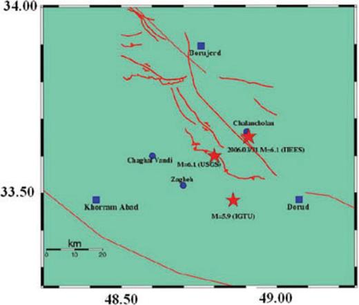
Map of the earthquakes location of the 2006 Silakhor, M_L = 6.1 and stations at which causative main shock were recorded.

Open in new tabDownload slide

Figure 6

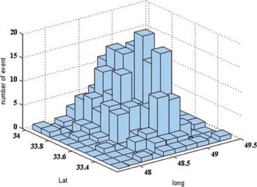
Distribution of the 2006 Silakhor earthquake aftershocks versus the variation of longitude and latitude of aftershocks (after Teimouri 2006).

Open in new tabDownload slide

Figure 7

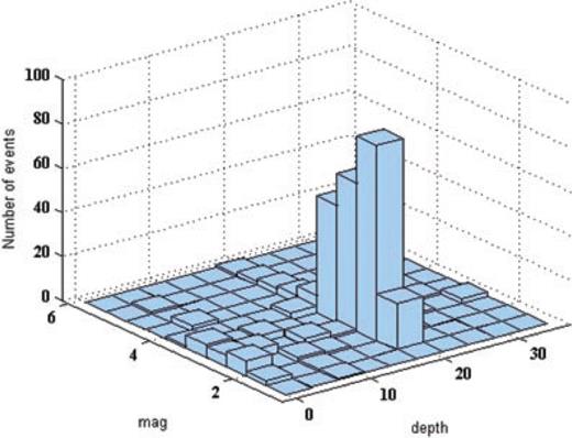
Distribution of the 2006 Silakhor earthquake aftershocks versus the variation of magnitude and depth (after Teimouri 2006).

Open in new tabDownload slide

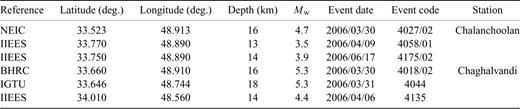
The recorded accelerogram in the Chalanchoolan station, with an S–P time of about 1.71 s is the closest available accelerogram, which suggests a focal distance of about 12 km. The maximum acceleration was recorded in the Chalanchoolan station with peak value of about 432 and 524 cm s⁻² on horizontal and vertical components, respectively. Seven foreshocks have been recorded. The strongest foreshock was that happened on Tuesday of 2006 March 30, at 19:36:16 (UTC). The station names, locations, horizontal waveform components, orientation and the number of recorded aftershocks during 2006 Silakhor Earthquake are listed in Table 1.

10 Model Validation, Results and Discussion

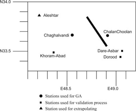
Table 2 lists the codes, dates and stations at which the aftershocks have been recorded during the 2006 Silakhor earthquake. The two selected stations, Chalanchoolan and Chaghalvandi, each of which with three components of aftershock records (L, T and V), are selected for calibration purpose as the first step. The other three stations, Dorood, Khoram-Abad and Dare-Asbar, at which the three components of the main shock have also been recorded, are selected for validation. Fig. 8 shows the stations surrounding the Silakhor earthquake epicentre at which both the main shock and aftershocks have been recorded.

Table 2

EGFs used for simulating the strong motion at Chalanchoolan and Chaghalvandi stations.

Open in new tabDownload slide

Figure 8

Location of causative fault and stations surrounding the Silakhor earthquake epicentre at which the main shock and aftershocks have been recorded.

Open in new tabDownload slide

The FORTRAN computer program ‘EMPSYN’ originally written by Hutchings (1988) is used in this paper. The well-known Kostrov slip function is used by which variable slip, rise time and healing phases in time domain are modelled, is used. The Kostrv slip function provides a good first-order approximation of the slip and rise-time based on the rupture velocity and distance from centre of the nucleation point location. In this paper, the procedure was performed similar to Hutchings et al. (2007). The hypocentre on the fault plane is found through thousands calculation performed by the GA technique. Fig. 9 shows the estimated slip and rise-time distribution throughout the fault area associated with the hypocentre location. The seismological model parameter values are optimally estimated through million's chromosomes (i.e. simulation estimation), error function calculations and model parameters minimization processes.

Figure 9

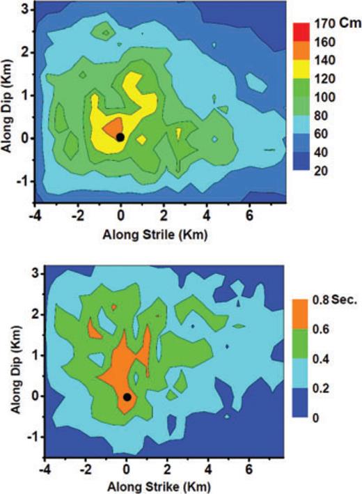
Estimated slip (up) and rise-time (down) distributions using Kostrov slip function distribution. The black circle shows the estimated hypocentre location on the fault plan.

Open in new tabDownload slide

The input parameters incorporated in the GA technique were as follows, the range of frequencies 0.2–20 Hz, the upper–lower bounds of hypocentre location and fault mechanism (strike, dip and rake angle) previously reported by BHRC, IGTU, NEIC, IIEES and Harvard CMT (see Table 3), and the upper–lower bounds for rupture length and width considered to be 130 –70 per cent times that of the empirical relationships proposed by Wells & Coppersmith (1994). The GA starts with two different population sizes of 50 and 100 chromosomes. The crossover and mutation rate for calculating the minimized error function within each chromosome were taken as 0.8 and 0.08, respectively. Three-point crossover together with a roulette wheel selection was taken into account. The number of bits for each chromosome was set to nj = 8. Finally, the maximum number of generations used as the termination criterion was ng = 50.

Table 3

Comparison illustration of the mainshock source information and focal mechanism used through this study and those of other references.

Open in new tabDownload slide

The aftershocks used in the two steps, calibration and prediction processes, were denoised using the aforementioned wavelet-based method. The six earthquake components recorded at the two stations, Chalanchoolan and Chaghalvandi, were selected for simulation process. The optimal values of seismological model parameters, epicentre coordinate, focal depth, focal mechanism (strike, dip and rake), rupture length and width were estimated in this step. The findings in the first step were incorporated in the model and the waveforms at the other three stations (Dorood, Dare-Asbar and Khoram-Abad) were predicted. The calculation process was stopped as long as the minimum errors corresponding to the best chromosomes were achieved (see Fig. 10). As is seen, the curve becomes asymptotic to a horizontal line showing the adequacy of calculation run. The figure also shows that the GA with population size 100 ends with effectively better convergence while suffering from heavier computational cost.

Figure 10

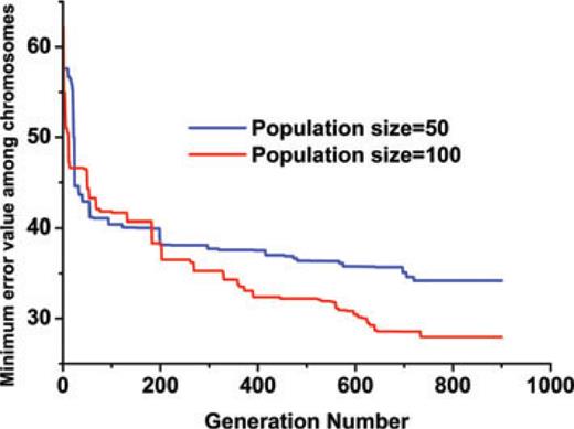
Minimum Error values in each generation for the two GA runs with different population sizes.

Open in new tabDownload slide

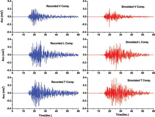
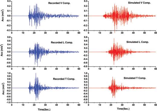
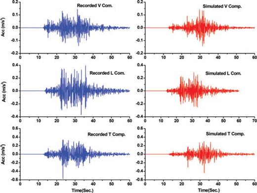
Figs 11 and 12 show comparison of the simulated acceleration time histories and those of the recorded data at the selected stations. Comparison of elastic response spectra and Fourier spectral amplitudes corresponding to the simulated and recorded waveforms are depicted in Figs 13 and 14. Good agreement of the synthetic and observed data confirms the applicability and reliability the proposed technique in a simulation realistic seismogram.

Figure 11

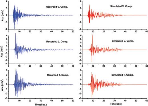
Synthesized and observed strong motions recorded at Chalanchoolan station.

Open in new tabDownload slide

Figure 12

Synthesized and observed strong motions recorded at Chaghalvandi station.

Open in new tabDownload slide

Figure 13

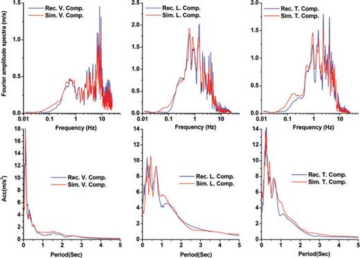
Comparison illustration of the elastic response spectra, with 5 per cent damping ratio, and the Fourier spectral amplitudes corresponding to the synthesized and recorded seismograms at Chalanchoolan station.

Open in new tabDownload slide

Figure 14

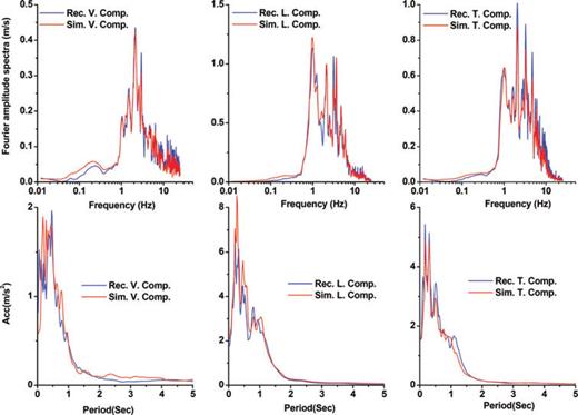
Comparison illustration of the elastic response spectra, with 5 per cent damping ratio, and the Fourier spectral amplitudes corresponding to the synthesized and recorded seismograms at Chaghalvandi station.

Open in new tabDownload slide

The validation process is done by predicting the three components of the mainshock earthquake (L, T and V) recorded at the other three stations, Dorood, Dare-Asbar and Khoram-Abad using the seismological model parameters found in the first step. Figs 15–17 demonstrate comparison of predicted waveforms and those of the observed seismograms at these three stations. The response spectra corresponding to the predicted and recorded seismograms at these stations are monitored in Fig. 18. Finally, Table 4 shows the estimated hypocentre location and fault dimensions of the causative fault. In addition, we predicted the three component recordings at the station Aleshtar, at which the aftershocks have not been recorded, using the EGFs recorded at the Chaghalvandi station, 33 Km far away from this station (See Fig. 8). Actually the EGF is extrapolated to a location other than that from which it has been recorded. We have called this approach an ‘extrapolation technique’, the same phrase as has been used by (Wossner et al. 2002).

Figure 15

Predicted synthetic waveforms and observed strong motions at Dorood station.

Open in new tabDownload slide

Figure 16

Predicted synthetic waveforms and observed strong motions at Dare-Asbar station.

Open in new tabDownload slide

Figure 17

Predicted synthetic waveforms and observed strong motions at Khoram-Abad station.

Open in new tabDownload slide

Figure 18

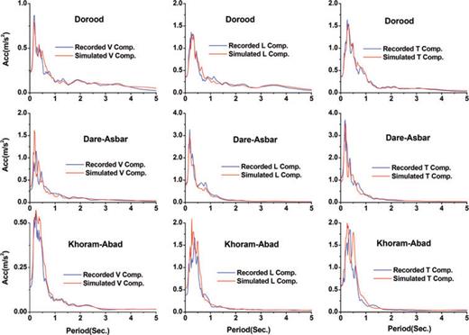
Comparison illustration of the predicted and synthesized elastic response spectra, with 5 per cent damping ratio, at Dorood, Dare-Asbar and Khoram-Abad stations with those of the observed data.

Open in new tabDownload slide

Table 4

Estimated hypocentre location and causative fault dimensions.

Open in new tabDownload slide

Fig. 19 illustrates comparison of the observed and synthesized time histories and elastic response spectra (5 per cent damping ratio) corresponding to the observed and simulated waveforms at Aleshtar station. Again, good agreement between the synthetic and recorded data confirms the validity of the proposed technique. The results of this study are supposed to be used in seismic performance evaluation non-linear dynamic analysis of new and existing structures and also for hazard analysis in the Silakhor region, which suffers from lack of sufficient data.

Figure 19

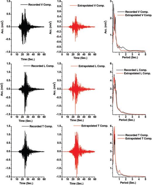
Comparison of the recorded and synthesized waveforms at Aleshtar station using the EGFs recorded at Cheghalvandi station.

Open in new tabDownload slide

11 Comparing the Results with those of Other Investigators

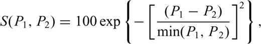
To demonstrate robustness of the proposed inversion solution technique we randomly selected a number of Silakhor fault plane data sets whose values are between those reported by other investigators (30 samples). The Error-Functions (eq. 7) resulted from incorporating these parameters were calculated and compared with those of our technique. Table 5 lists the selected hypocentre locations, strikes, dips and rakes proposed by the investigators (Table 3) and those of this study. The calculated error values associated with those of the others are depicted in Fig. 20 from which the differences between error values are quite visible.

Table 5

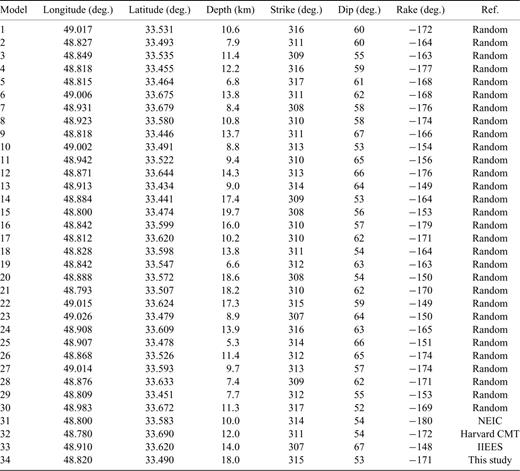
Randomly selected Silakhor fault plane and focal mechanism information, extracted from Table 3, and those of this study.

Open in new tabDownload slide

Figure 20

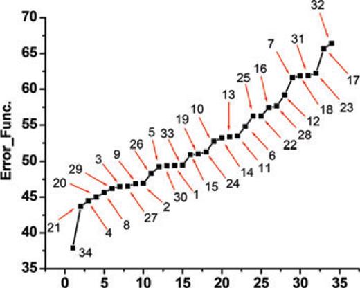
Comparison illustration of error values (eq. 7) calculated from incorporating randomly selected 33 sets of parameters in the model and those of this study.

Open in new tabDownload slide

In addition, we predicted waveforms at Chalanchoolan and Cheghalvandi stations incorporating the fault plane information reported by other investigators (see Table 3) and compared the error values (eq. 7) corresponding to the elastic response spectra, with 5 per cent damping ratio, to those of this study (see Fig. 21). More agreement between this study and those of the observed data confirms the robust reliability of our results. Nevertheless, we do not claim that the error values reflect physically the accuracy of the parameters but rather demonstrate the effectiveness and reliability of our technique.

Figure 21

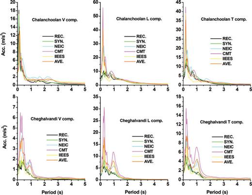
Comparison illustration of the elastic response spectra corresponding to the synthesized seismograms obtained from incorporating the model parameters previously reported by other investigators and those of this study. The references are listed in Table 3.

Open in new tabDownload slide

12 Summary and Conclusions

An EGF-based methodology for predicting spectrum compatible seismograms at sites at which main shock is not recorded from site where the main event has been observed is proposed using recorded aftershocks. A wavelet-based soft-thresholding approach is used for denoising the aftershocks with low SNR. The well-known MTM is employed which permits the reduction of spectral leakage which allows matching the Fourier spectral amplitudes corresponding to the synthesized and observed waveforms. The procedure is performed through a simulation process of EGF-based seismograms, a MTM and a GA. All three procedures were developed for optimizing the model parameter values. The proposed technique was applied to the 2006 Silakhor earthquake (M_w = 6.1), as a case study. We simulated the six components of waveforms during the 2006 Silakhor (Iran) earthquake at five stations using the above-mentioned procedure. The aftershocks were denoised before being used in the process using the aforementioned wavelet approach. Two stations were selected for calibrating the model, as the first step, and three stations for validation as the second step. The differences between the Multitapered Fourier spectral amplitudes and response spectra corresponding to the two sets of signals, six components of synthesized and waveforms (L, T and V), are minimized. Relatively good agreement between the calculated synthetic seismograms and those of observed data at the first step confirms the validity and suitability of the model parameters. The findings from the first step were incorporated in the model and the seismograms at the other three stations were predicted. Again, a good match of the response spectra and Fourier spectral amplitudes corresponding to the predicted and observed data confirms the robust reliability of our methodology in predicting the spectrum compatible acceleration time histories in the region under study. Furthermore, we predicted the recordings at the Aleshtar station at which the aftershocks have not been recorded, using EGFs recorded at another station (Cheghalvandi), which resulted in good agreement with those of the observed data. It is worth that we do not claim that our technique is able to estimate the actual physical source parameter values that the results of this research work are free from uncertainties. Nevertheless, the methodology can be used for the predicting the realistic seismograms for compensating the required waveforms for seismic performance of structures in regions, which lack sufficient, reliable data. We believe that the whole methodology needs more work at least in phase and polarity parts of the problems. The proposed technique can also be used in site-specific studies, linear and non-linear dynamic analysis of important structures and the retrofitting process of existing important buildings in the Silakhor region.

Acknowledgments

Our sincere thanks go to Profs. L.J. Hutchings and Profs. G.A. Prieto, for kindly offering the valuable codes and Dr. Y. Fahjan for giving windows EMPSYN FORTRAN Codes. We also thank BHRC for giving the valuable information of Silakhor earthquake.

References