A parametrization study for surface seismic full waveform inversion in an acoustic vertical transversely isotropic medium

Summary

1 Introduction

By minimizing the error misfit between modelled and observed data, full waveform inversion (FWI) may produce more accurate images of the subsurface than the traditional traveltime tomography. After its introduction in the 1980s (Lailly 1983; Tarantola 1984; Gauthier et al. 1986; Mora 1988; Tarantola 2005), several studies have been published in seismology and exploration geophysics showing the relevance and the difficulties of FWI (Sun & McMechan 1992; Pratt et al. 1996; Pratt 1999; Shipp & Singh 2002; Dessa et al. 2004; Ravaut et al. 2004; Brenders & Pratt 2007). With the increase of computer power, real-sized 3-D applications have also been reported (Epanomeritakis et al. 2008; Fichtner et al. 2009; Plessix 2009; Plessix & Perkins 2010; Sirgue et al. 2010; Vigh et al. 2010).

FWI is an ill-posed problem and one cannot retrieve all the Earth elastic parameters by inverting seismic data. Depending on the nature of the seismic data sets we want to invert, one often applies some approximations and defines a hierarchical procedure to first retrieve the most important parameters (Tarantola 1986; Pratt et al. 1996; Shipp & Singh 2002). With active surface seismic data generated by a pressure source or a vertical displacement source, one commonly assumes an acoustic wave propagation. While this assumption is relevant to model the kinematics of the compressional waves, it is not satisfactory to interpret the dynamics of the reflection data that significantly depends on the elastic properties of the Earth. One remedy is to apply a scale separation: to decompose the Earth parameters into propagation and reflectivity, and to consider acoustic propagation with elastic reflectivity. The first step is to retrieve a macro (background) acoustic model that explains the kinematics of the compressional waves. This approach is notably applied to obtain a structural depth image. The compressional waves are favoured because they have a deeper depth penetration than the shear waves. This often means that the data should be carefully pre-processed to mitigate the shear events (Plessix et al. 2010). To avoid the acoustic assumption, a more realistic elastic inversion can be carried out (Tarantola 1986; Mora 1988; Sun & McMechan 1992; Shipp & Singh 2002; Sears et al. 2008; Brossier et al. 2009; Lee et al. 2010). This however increases the number of parameters to invert for and further complicate the non-linear inversion approach (Tarantola 1986; Brossier et al. 2009; Lee et al. 2010). Since we minimize the FWI misfit functional with a local optimization technique due to the large computational cost of forward modelling, this means that we have more chances to end up in a local minimum when we carry out an elastic inversion. Several authors have then proposed a hierarchical approach where we first invert for the dominant parameters and estimate the different parameters in a sequential manner (Tarantola 1986; Brossier et al. 2009). With single component data sets generated by a pressure or a vertical displacement source, this often means to first carry out an acoustic inversion.

Hence, estimating an acoustic macromodel often constitutes the first step in our analysis sequence. In FWI, this can be achieved by using an elastic modelling approach and imposing a certain relation between the compressional and shear velocities. This can also be achieved by using an acoustic modelling approach. Both approaches have the same model space dimension. The first approach has the advantage to allow more realistic physics and to a priori better model the dynamics of the reflection waves. It is however much more computationally expensive. Indeed, 3-D elastic inversion of active-source data sets containing thousands to hundreds of thousands of shot points is rarely affordable on the current computers. In this paper, we shall then discuss the acoustic FWI in the context of macromodel building. An important application of this work is the inversion of active surface marine (streamer, Ocean Bottom Seismometer or Ocean Bottom Cable) data sets. Nevertheless, it can also be applied to active surface land seismic data sets (Ravaut et al. 2004; Plessix et al. 2010). To update the macromodel with FWI, we invert both the short and long offsets of the data (Pratt et al. 1996; Shipp & Singh 2002; Ravaut et al. 2004; Brenders & Pratt 2007). The isotropic assumption is often insufficient to explain the kinematics of the short and long offsets. It was shown that FWI leads to better results when some anisotropy is taken into account (Barnes et al. 2008; Plessix 2009; Lee et al. 2010; Vigh et al. 2010). The simplest anisotropy to consider is the vertical transversely isotropic (VTI) one. Although pure acoustic anisotropy does not exist in the Earth, acoustic VTI wave equations have been proposed by several authors (Alkhalifah 1998; Alkhalifah 2000; Zhou et al. 2006;
Duveneck et al. 2008; Operto et al. 2009). These equations give a correct estimation of the kinematics of the P waves and of the dynamics of the long-offset diving P waves. They therefore seem to be appropriate for FWI in the context of macromodel building. The acoustic VTI wave equations depend on four parameters: three parameters to define the stress–strain relation and density. In an acoustic VTI medium and using the Voigt notation, the stress–strain tensor, C, can be defined by the parameters C₁₁, C₃₃ and C₁₃, since we have C₁₂=C₁₁ and C₂₃=C₁₃. Because it is often not possible to retrieve all Earth parameters from seismic data, the parametrization of the inverse problem is important (Tarantola 1986). With surface seismic data, especially when only one component (generally pressure or vertical displacement) is taken into account, one cannot retrieve the three stress–strain components without additional information (Banik 1984; Banik 1986; Tsvankin & Thomsen 1994; Alkhalifah & Tsvankin 1995; Grechka & Tsvankin 1998; Plessix & Bork 2000; Kiyashchenko et al. 2004).

Thomsen (1986) parametrized the VTI stress–strain relation with the vertical velocity , with the density, ρ and two dimensionless parameters ɛ= (C₁₁−C₃₃) /(2C₃₃) and δ= (C²₁₃−C²₃₃)/(2C²₃₃). The parameter ɛ relates the horizontal velocity, v_h, to the vertical velocity, .
Alkhalifah & Tsvankin (1995) have shown that the traveltime curve of the P-wave reflection could be parametrized by two parameters: the NMO velocity, , and the anelliptic parameter η= (ɛ−δ)/(1 + 2δ) (the η parameter could be replaced by the horizontal velocity). Because this result is valid at all offsets, this indicates that the two main parameters for acoustic VTI FWI in the context of macromodel building are the NMO velocity and the η parameter (or the horizontal velocity) (Alkhalifah et al. 2001). From a kinematic point of view, density does not play a role and its effect may then be accounted for only after an estimate of the propagation parameters is recovered (Tarantola 1986).

In this paper, based on those observations, we study the parametrization of the acoustic VTI FWI and the acoustic kinematic parameters we can retrieve. Some preliminary studies have also been done in an elastic VTI medium (Gholami et al. 2010a; Gholami et al. 2010b; Lee et al. 2010). We first discuss a formulation of the VTI wave equations with the NMO velocity, the η parameter and a NMO pressure field equal to times the vertical stress. The analysis is based on a change of coordinates that is related to the one presented in Alkhalifah et al. (2001). However, here we just apply a depth stretching without going to the vertical time and we work with the first- and second-order formulations of
 the VTI wave equations (Duveneck et al. 2008). We also illustrate the ambiguity between the depth and the δ parameter through modelling examples. In the third section, we apply an eigenvector/eigenvalue decomposition analysis of the Hessian of the least-squares misfit functional to further study the parametrization of FWI. In the fourth section, we illustrate the results with synthetic FWI examples. We complement the paper with several appendices to describe more precisely the gradient computation under the acoustic VTI assumption and its relations with migration. We also describe an approach for the source estimation.

2 Parametrization of the Acoustic VTI Wave Equation

FWI consists of minimizing the misfit between the observed data, d, and the computed, synthetic data, c (Tarantola 2005). The synthetics are solutions of the wave equation and depend on the earth model parameters m. The least-squares inverse problem is formulated as follows: Find m^opt such that m^opt minimizes the misfit
 functional

1

Here, c and d are vectors representing multishot, multireceiver data sets depending on time or frequency, W is a data diagonal correlation (weight) matrix and ^T denotes the (complex) transpose. The functional f_reg is a model regularization term (for simplicity, we will ignore it in the rest of this paper).

As pointed out by many researchers, we cannot retrieve all the Earth elastic parameters from seismic data. The inverse problem is an ill-posed problem. In this work, we consider the VTI case and discuss which background parameters can be retrieved by FWI. By background parameters, we mean the parameters that influence the kinematics of the waves. We want to retrieve the long wavelengths of those parameters.

The kinematics of the compressional waves are correctly estimated with the acoustic VTI wave equations obtained by zeroing the vertical shear velocity in the stress–strain relation (Alkhalifah 1998, 2000; Zhou et al. 2006; Duveneck et al. 2008). Alkhalifah & Tsvankin (1995) have shown that the kinematics of the body waves depends only on the NMO velocity, v_n and the η parameter. To study the main kinematics parameters in the FWI approach, we therefore write the VTI wave equations in terms of v_n, η, δ and density ρ. 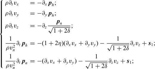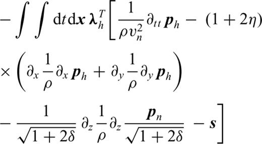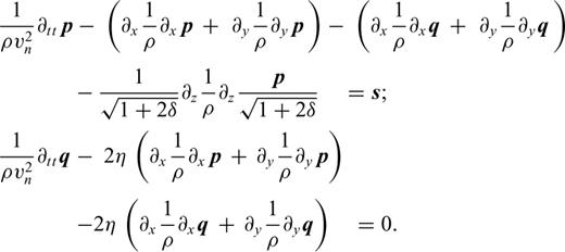We define the ‘horizontal’ and ‘vertical’ pressures, p_h and p_v, as minus the horizontal and vertical stresses and we introduce the field , called NMO pressure. Starting with the equations described in Duveneck . (2008) the second-order acoustic VTI wave equations read, with s an isotropic source term

2

with the initial conditions

Absorbing boundary layers are implemented for the numerical examples, expect for the top of the model where a free surface boundary condition can be imposed. The medium around the source and the receivers is assumed isotropic to avoid shear artefacts (Grechka et al. 1994). In an isotropic medium, η= 0, and p_h=p_n. We compute the synthetics, c, with the sampling operator S and α₁+α₂= 1 by c=S(α₁p_h+α₂p_n). Since we have p_h=p_n at the receiver locations, this general expression could be replaced by c=Sp_n or
c=Sp_h or .

The use of the NMO pressure p_n allows us to limit the dependence on δ to the terms with vertical derivatives. Similarly to the change of coordinates between depth and vertical time (Alkhalifah 2001), we can define the following change of coordinates:

3

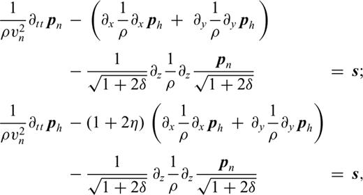
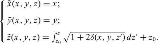
Here, z₀ is the depth origin and is the stretched depth that depends on the lateral coordinates.

Assuming a smooth δ field and neglecting the derivatives of δ with respect to the more oscillatory derivatives of the pressure fields, the system (2) can be approximatively rewritten as follows (see also Appendix A)

4

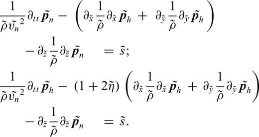
The variables with a tilde are function of and .

With a smooth δ parameter, this change of coordinates shows the known ambiguity between δ and depth since system (4) does not depend on δ. This ambiguity cannot be resolved by inverting surface seismic data under an acoustic VTI assumption even with long offsets (Alkhalifah & Tsvankin 1995). In practice, δ can be inferred from the amount of depth stretching required to tie the depth of the migrated section to the depth in the wells.

With η= 0, the system (4) is the isotropic equation

5

with p the pressure and v the (isotropic) velocity.

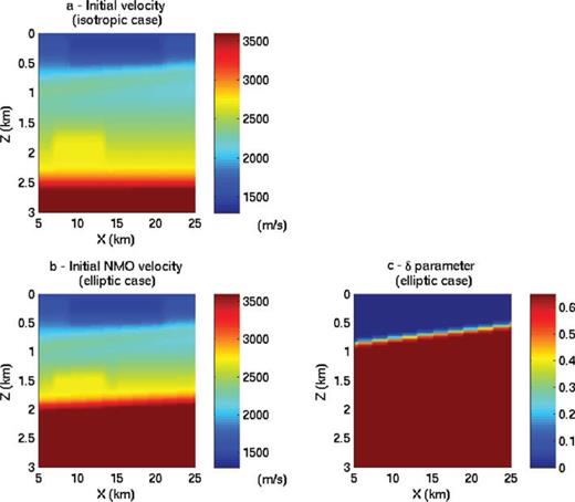
To illustrate the ambiguity between δ and depth, we compare a seismogram computed in an elliptic Earth with three seismograms computed in an isotropic Earth. For the elliptic case, we solve the acoustic VTI wave equations (2) with the NMO velocity and the δ parameter displayed in Figs 1(c) and (b). We impose η= 0. For the isotropic cases, we solve the isotropic eq. (5) with

Figure 1

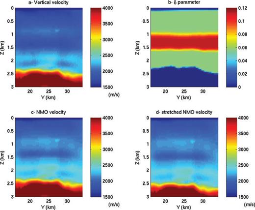
Models for the time-domain modelling study. The vertical velocity (a) and the δ parameter (b) define an elliptical anisotropic model. The NMO velocity (c) is obtained by multiplying the vertical velocity by . The stretched NMO velocity (d) is obtained from the NMO velocity after having stretched the depth axis using the change of variables written in eq. (3).

Open in new tabDownload slide

• (i)

  The velocity equals the vertical velocity displayed in Fig. 1(a).

• (ii)

  The velocity equals the NMO velocity displayed in Fig. 1(c).

• (iii)

  The velocity equals the stretched NMO velocity displayed in Fig. 1(d). This stretched NMO velocity is obtained from the NMO velocity by the change of variables described in eqs (3). We can see that the velocity boundaries after 1.5 km depth have been shifted down.

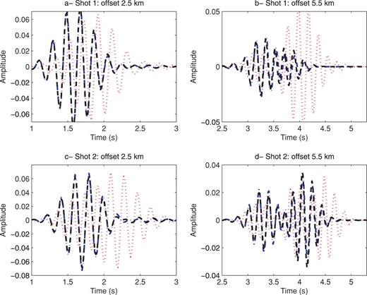
The seismograms are displayed in Fig. 2. The seismogram computed in an isotropic Earth with the stretched NMO velocity is the only one in phase with the seismogram computed in an elliptic Earth. As expected, there are small amplitude differences because the spatial derivatives of the δ parameter cannot be neglected at the discontinuities. However, this result shows that the elliptic modelling can be mimicked with an isotropic modelling and a proper depth stretching.

Figure 2

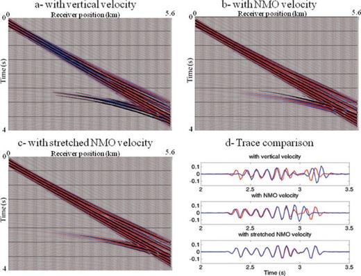
Comparison between seismograms computed in an elliptic Earth and an isotropic Earth. In graphs (a), (b) and (c), the seismogram computed in an elliptic Earth is displayed in colour in the background. The seismograms display with black wiggles are computed in an isotropic Earth with the vertical velocity (a), the NMO velocity (b) and the stretched NMO velocity (c). The seismograms are in phase when the black loop matches the red loop. On graph (d), the blue curve corresponds to the trace at 4.3 km offset computed in the elliptic Earth and the red curve in an isotropic Earth.

Open in new tabDownload slide

In Appendix B, the influence of a laterally varying δ parameter is numerically studied. This appendix illustrates that the trade-off between depth and δ parameter also exists with diving waves.

From this analysis, we conclude that δ and density play a smaller role than NMO velocity and η when FWI focuses on retrieving the background velocity.

3 Eigenvector Decomposition Analysis

To analyse which earth model parameter can be retrieved by FWI, we can also carry out an eigenvector/eigenvalue decomposition of the Hessian of the least-squares misfit.

The least-squares functional, J, is linearized around a given model m

6

where δm is the model perturbation, g is the gradient, the first derivative of J and H is the Hessian, the second derivative.

The minimum of J_lin satisfies Hδm=−g. The symmetric matrix H can be decomposed into

7

with Λ the eigenvalue matrix and R the eigenvector matrix. The components of eigenvectors are called direction cosine.

The direction cosines of the normalized eigenvector, r_i, associated with the eigenvalue, λ_i, give the relative importance of the model parameters. By studying those direction cosines, we shall then determine the combination of the model parameters related to the eigenvalue, λ_i. In an inversion process, the most reliable information is associated with the largest eigenvalues.

We start with two elementary cases and then analyse a more complex case. In the first case, the data misfit is dominated by diving waves, in the second case (pre-critical reflection case), the data misfit is dominated by reflected waves. For simplicity, we consider absorbing boundary conditions on all the edges of the domain. We also display maps of the misfit functional.

3.1 Diving wave case

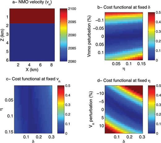
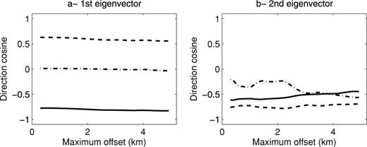
In this diving wave case, the Earth model, Fig. 3(a), consists of a velocity gradient and a perturbation with the size of a few wavelengths. The source is located on the top left corner and we consider 12 km offset. The main frequency in the data is 5 Hz. The perturbation corresponds to a ball of about 3 km in diameter; the edges have been smoothed to reduce the reflection effects. It is an anisotropic perturbation. This case differs from the ‘classical’ diffraction case because the perturbation is spatially large. Because of the velocity gradient, diving waves are recorded. These diving waves travel through the perturbation. We now study the least-squares misfit functional when the Earth parameters change in the ball. In Figs 3(b)–(d), we plotted three slices of the misfit functional. The misfit functional is far less sensitive to a perturbation of δ than to a perturbation of NMO velocity or η. We also note the trade-off between NMO velocity and η, Fig. 3(c), since the graph shows an elongated shape in the diagonal direction. With the parametrization v_n and η, the first eigenvector of the Hessian (Fig. 4) is mainly related to and Δη, with almost equal weights. These two results indicate that the most sensitive combination of parameters is approximately . That means . We confirm this result by computing the eigenvectors of the Hessian using the parametrization v_n and v_h (Fig. 5). The first eigenvector is now mainly related to v_h, especially at long offsets.

Figure 3

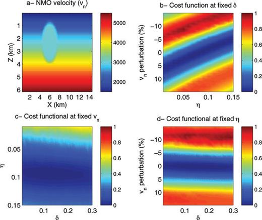
Slices of the misfit functional with diving waves only. In graph (a), a typical NMO velocity with a velocity gradient and a large perturbation is displayed. Three slices of the misfit functional are plotted when the values of the large perturbation are modified, in graph (b) when the δ parameter is kept fixed, in graph (c) when the NMO velocity, v_n, is kept fixed, and in graph (d), when the η parameter is kept fixed.

Open in new tabDownload slide

Figure 4

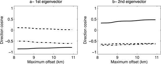
First and second eigenvectors of the Hessian computed in the model displayed in Fig. 3 with the parametrization v_n, η, and δ. The solid line corresponds to and the dot–dashed line to Δη and the dashed line to Δδ.

Open in new tabDownload slide

Figure 5

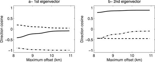
First and second eigenvectors of the Hessian computed in the model displayed in Fig. 3 with the parametrization v_n, v_h, and δ. The solid line corresponds to , the dot–dashed line corresponds to and the dashed line corresponds to Δδ.

Open in new tabDownload slide

This small study illustrates that the diving waves mainly depend on the horizontal velocity and are not influenced by δ in the parametrization v_n, v_h and δ. This is in agreement with the findings of the previous section.

3.2 Reflection wave case

In this reflection wave case, the earth model is constituted by two half-spaces (Fig. 6). The first half-space is fixed during the analysis. The source and receivers are 1.5 km above the interface in the first half-space; the maximum offset is 5 km. By varying the Earth parameters in the second half-space, we analyse the effects of the reflections in the misfit functional. This is similar to the amplitude versus offset analysis discussed in Plessix & Bork (2000). Three slices of the misfit functional are displayed in Figs 6(b)–(d). The misfit functional is mainly sensitive to NMO velocity and δ. We notice a trade-off between NMO velocity and δ, Fig. 6(d). The first eigenvector of the Hessian using the parametrization v_n, η, and δ, as displayed in Fig. 7, also shows that the most sensitive parameter is the combination of parameters that is almost equal to . This means , with , the vertical velocity. This result is not surprising since the zero-offset reflection coefficient is equal to . This result is also in agreement with the findings of the previous section because δ plays a role in the dynamics of the reflected waves.

Figure 6

Slices of the misfit functional with reflected wave only. In graph (a), a typical NMO velocity with a velocity gradient and a large perturbation is displayed. Three slices of the misfit functional are plotted when the values of the large perturbation are modified, in graph (b) when the δ parameter is kept fixed, in graph (c) when the NMO velocity, v_n, is kept fixed, and in graph (d), when the η parameter is kept fixed.

Open in new tabDownload slide

Figure 7

First and second eigenvectors of the Hessian computed in the model displayed in Fig. 6 with the parametrization v_n, η, and δ. The solid line corresponds to , the dot–dashed line corresponds to Δη and the dashed line corresponds to Δδ.

Open in new tabDownload slide

3.3 A more complex case

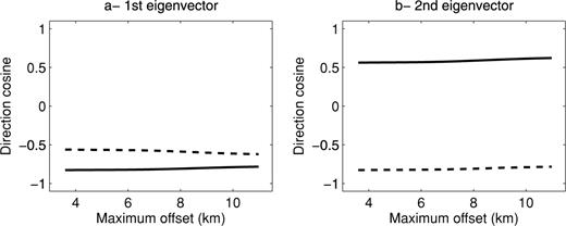
We now consider a case where pre- and post-critical reflected waves, together with diving waves, are recorded in the data set. The earth model is displayed in Fig. 8. We assume a streamer acquisition. Keeping the δ parameter fixed, we compute the eigenvectors versus maximum offset in the parametrization v_n and η (Fig. 9) and in the parametrization v_n and v_h (Fig. 10). The first eigenvector mainly corresponds to . The second eigenvector almost corresponds to . The ratio between the eigenvalues is around 50, meaning that the first combination of parameters shall have much larger sensitivity. This result differs from the one obtained with the diving wave case because in the first eigenvector, the weight of v_n in the parametrization v_n, v_h, does not decrease when the maximum offset increases. This could be due to the influence of the reflection waves. Indeed, the kinematics of the reflection waves dominantly depends on the NMO velocity (Grechka & Tsvankin 1998). In this study, we decided to perturb the whole model with the same percentage when computing the Hessian in order to have only two models parameters. The result may be a bit different from a layered approach. Moreover, the results may depend on the amplitude ratios between the different waves. Nevertheless, this result indicates that a mono-parameter FWI (mainly an isotropic FWI) will probably give a velocity that has values between the NMO velocity and the horizontal velocity. This was noticed on some real FWI examples (Plessix & Perkins 2010; Plessix & Rynja 2010). This also means that FWI may return a slightly faster (NMO) velocity for migration when anisotropy is ignored, since the horizontal velocity is often a bit faster than the NMO velocity. This result, together with the one obtained with the diving wave case, shows that the parametrization v_n, v_h is slightly better than the parametrization v_n, η. This however needs to be confirmed with more numerical examples.

Figure 8

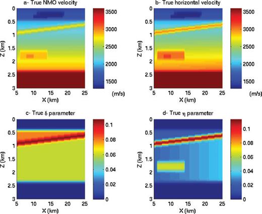
VTI Earth parameters used to generate the synthetic example.

Open in new tabDownload slide

Figure 9

First and second eigenvectors of the Hessian computed in the model displayed in Fig. 8 with the parametrization v_n and η. The solid line corresponds to and the dashed line to Δη.

Open in new tabDownload slide

Figure 10

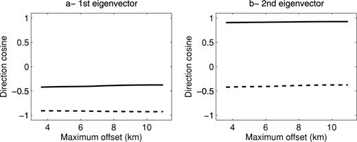
First and second eigenvectors of the Hessian computed in the model displayed in Fig. 8 with the parametrization v_n and v_h. The solid line corresponds to and the dashed line to .

Open in new tabDownload slide

4 Numerical Examples

We continue the study with some synthetic anisotropic FWI. A real example has been presented in Plessix & Rynja (2010). In our approach, we minimize the misfit functional with a quasi-Newton optimization. The gradient is computed with the classic adjoint-state technique (Chavent 1974; Plessix 2006). The inverse of the Hessian, the second derivative of the misfit functional, is approximated during the iterations with a limited memory BFGS method (Nocedal & Wright 2006). The initial approximation of the inverse of the Hessian is a diagonal matrix. The diagonal values are the inverse of the Born approximation of the Hessian computed in a constant medium (Plessix & Mulder
 2004).

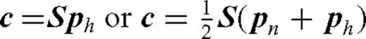
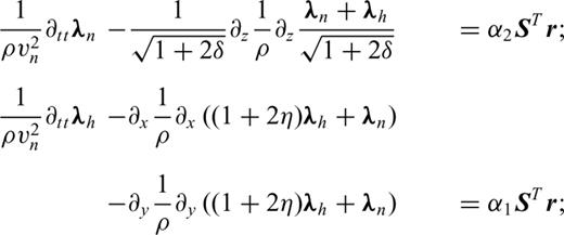
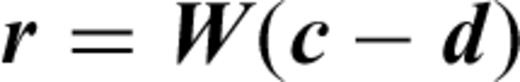
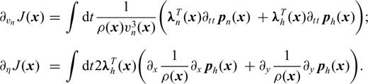
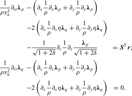
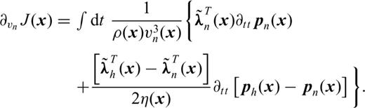
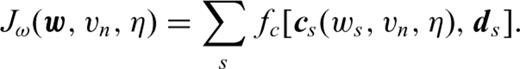
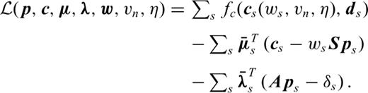
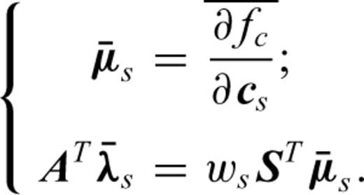
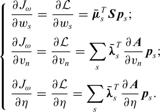
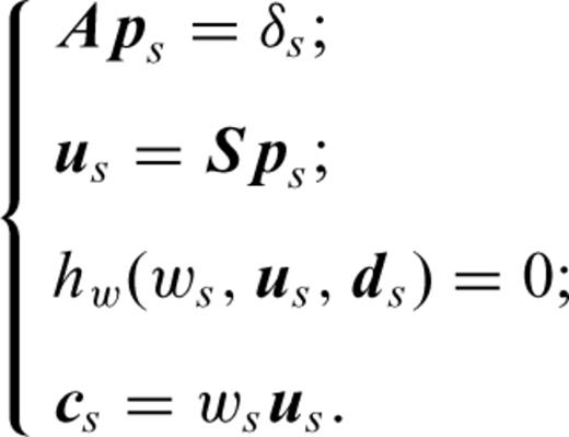
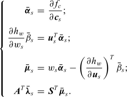
We adopt a frequency-domain formulation of FWI (Pratt et al. 1996). In the frequency-domain, the discretization of the wave eqs (2) leads to a linear system Ap=s, with A the matrix of the discrete wave operator, p the vector of the discrete values of p_h and p_n and s the source term. The synthetics c are obtained by sampling p onto the receiver positions, c=Sp, with s the sampling operator. In the frequency domain, the adjoint (backward) system is simply A^Tλ=
S^TW(c−d) with λ the adjoint or backpropagated field and ^T the complex transpose (W is the data correlation matrix and d the observed data). The gradient of the misfit functional, eq. (1), with respect to a model parameter m, is given by ∂_mJ=λ^T∂_mAp.

We could show similar results with a time-domain approach. However, the computation of the gradient with a time-domain acoustic VTI approach is slightly more complicated because the formulation is often not self-adjoint. In the Appendix C, we briefly describe a time-domain formulation and also discuss the imaging principle under acoustic VTI assumption.

To solve the linear system, we use a 3-D iterative solver as described in Erlangga et al. (2006), Plessix (2007). For these examples with a 2-D geometry, a 2-D direct solver would lead to a faster
 approach. However, the 3-D iterative solver allows us to invert
 3-D data sets in a few days on sufficiently large computer
 clusters (Plessix 2009; Plessix & Perkins 2010; Plessix & Rynja
 2010).

4.1 Data and inversion set up

We generate a VTI synthetic data set from the model displayed in Fig. 8. A free surface boundary condition is used. This is a shallow water example with 150 m of water. The velocity and η parameter contain some smooth lateral variations. The velocity also contains a shallow low velocity zone. The acquisition geometry mimics a streamer acquisition with 321 shots and a maximum offset of 6 km.
 The shot spacing is 75 m. We invert the frequencies 4.5 and
 5.4 Hz sequentially in a classical multiscale approach. We carry out 15 iterations per frequency. At each iteration, a source wavelet per shot is also estimated (see Appendix D). This acquisition is a typical streamer acquisition and we hope to be able to retrieve the long wavelengths of the Earth parameters up to 1.5 or 2 km depth.

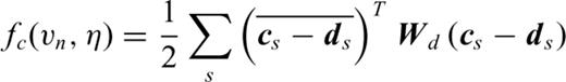
In the misfit functional J, eq. (1), the data weights W are used to balance the energy between the short and the long offsets. In the examples, we use the square root of the offset as data weights.

Although, the examples have a 2-D geometry, we ran 3-D inversions. At each iteration, the gradient is smoothed with a Gaussian filter. This is a simple approach to reduce some high frequency artefacts that may appear during the gradient computation. In the examples, we used a 100 m × 100 m × 50 m discretization grid, and a Gaussian smoother with a length of 300 m in the inline direction, 700 m in the crossline direction and 100 m in depth.

4.2 Acoustic isotropic versus elliptic FWI

Here we carry out two inversions: an isotropic inversion and an elliptic inversion. The initial velocity models were derived by smoothing the true NMO velocity. We also compensate for the δ stretching with the change of variables described in eq. (3). The initial Earth parameters are displayed in Fig. 11. For the elliptic case, we consider a non-constant δ parameter that is rather different from the true one. The isotropic and elliptic initial values give almost the same synthetic seismograms (Fig. 12). The main difference is in amplitude due to the discontinuities in δ (Fig. 11c).

Figure 11

Initial velocities for the isotropic FWI, graph (a), and for the elliptic FWI, graph (b). The δ parameter for the elliptic inversion is displayed in
 graph (c).

Open in new tabDownload slide

Figure 12

Comparisons between the traces computed with the true VTI velocities (red dotted lines), the traces computed with isotropic initial velocity (blue dash–dotted lines), and the traces computed with the elliptic initial traces (black dashed–dashed lines). The shot 1 is located on the horizontal axis at 15 km and the shot 2 at 22 km.

Open in new tabDownload slide

The inversion results are displayed in Fig. 13 together with the true NMO and horizontal velocities. The true velocities and the velocity after elliptic FWI have been stretched with the corresponding δ parameters. This allows us to compare the different results. The isotropic and elliptic FWI give very similar results. There are small differences at the discontinuities. These observations are in agreement with the previous sections where it was illustrated that the δ parameter does not really influence the kinematics of the waves but does modify the dynamics when it is discontinuous. The retrieved velocities are on average faster than the NMO velocities and slower than the horizontal velocities, indicating that FWI tries to compensate for anisotropy (the true η parameter is not equal to zero). This also probably explains the lateral variations (oscillations) in the FWI results since these variations will induce some anisotropy. This confirms the conclusions drawn after from eigenvector/eigenvalue decomposition analysis.

Figure 13

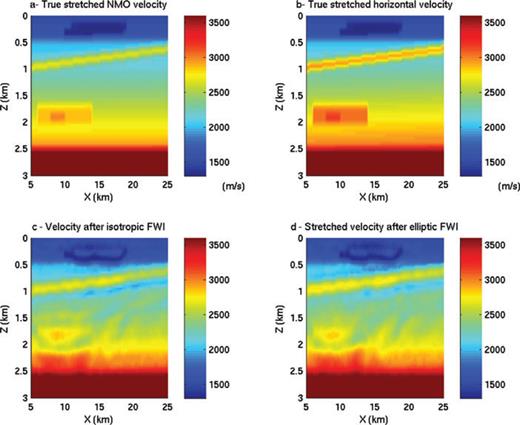
True NMO velocity, graph (a) and true horizontal velocity, graph (b), plotted in the stretched coordinate system for comparison with the isotropic results. Graph (c) displays the isotropic FWI result and graph (d) the elliptic FWI result in the stretched coordinate system.

Open in new tabDownload slide

In this example, acoustic FWI with low frequencies seems to mainly update the kinematics. In Fig. 12, we display a few time traces computed with the true VTI velocities, the initial isotropic velocity and the initial elliptic velocity. We notice some phase (time) errors between the modelling with the true and the initial velocities. The isotropic and elliptic initial velocities give seismograms that are in phase. In Fig. 14, we plot a few traces computed with the true VTI velocities and the isotropic and elliptic FWI results. The two
 inversions give similar seismograms. The retrieved traces are now more or less in phase with the true traces indicating that the kinematics is retrieved, however there are amplitude differences.

Figure 14

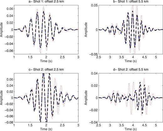
Comparisons between the traces computed with the true VTI velocities(red dotted lines), the traces computed with the isotropic FWI results (blue dash–dotted lines), and the traces computed with the elliptic FWI results (black dashed–dashed lines). The shot 1 is located on the horizontal axis at 15 km and the shot 2 at 22 km. The isotropic and elliptic FWI results are similar.

Open in new tabDownload slide

4.3 Acoustic anelliptic FWI

We now try to retrieve a second (kinematics) parameter by FWI. In this inversion, we fix the NMO velocity to the one retrieved by isotropic FWI and we assume that the δ parameter is equal to 0. We use the parametrization v_n and v_h and invert for v_h with v_n fixed. However, we display the η parameter. The starting η value is 0, meaning that v_h=v_n. The result is displayed in Fig. 15. The η parameter is not really retrieved, except in the shallow middle part. This could be explained by the limited offset range and by the ambiguities between velocity heterogeneities and anisotropy. By allowing the NMO velocity to vary on a 100 m scale in the isotropic inversion, we obtain a velocity with too much (short wavelength) variations (oscillations) compared to the true one. These variations, that are of the order of the wavelength, induce some anisotropy. In this way, the kinematics is correctly retrieved with only the isotropic velocity (see Fig. 14). With real data recorded over geological settings that exhibit anisotropy, unexpected short scale variations have also been noticed on velocity models retrieved by isotropic FWI (Plessix & Perkins 2010; Sirgue et al. 2010). Another explanation would be that FWI is blocked in a local minimum after isotropic FWI. The data comparison, Fig. 14, seems to indicate that it is not really the case. However, non-linearity is one of the main difficulties of FWI.

Figure 15

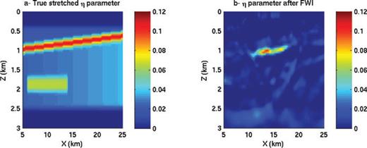
True, graph (a), and retrieved, graph (b), η parameters. The true η parameter is depth stretched for comparison. The retrieved η parameter was found by inverting for η assuming a fixed NMO velocity (the data set had 6 km offset).

Open in new tabDownload slide

4.4 Anelliptic FWI with 9 km offset

To see the influence of the long offsets, we now invert a data set with 9 km offset instead of 6 km. We first estimate the NMO velocity assuming an elliptic model (i.e. η= 0) starting from the smoothed NMO velocity plotted in Fig. 11. Then we invert for the horizontal velocity with the NMO velocity fixed at the value found in the first inversion. We display the retrieved η parameter in Fig. 16. The η parameter is now much better retrieved. Adding long offsets helps to resolve some of the ambiguities between velocity and anisotropy. Whereas 6 km offset was sufficient to retrieve a reasonable velocity model up to about 2 km depth, we needed 9 km to correctly estimate the anelliptic parameter η.

Figure 16

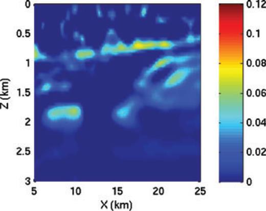
Retrieved η parameter after anelliptic FWI with a data set containing 9 km offset.

Open in new tabDownload slide

5 Conclusions

We studied the parametrization of the acoustic VTI FWI. Because of the acoustic assumption, we cannot correctly interpret the dynamic behaviour of the reflections that also depends on the elastic parameters. We therefore focus on the long wavelength updates of the Earth parameters that influence the kinematics of the waves. With a specific parametrization of the VTI wave equations, we could show that the kinematics is mainly governed by the NMO velocity and the η parameter (or equivalently the horizontal velocity). The long wavelength variations of the δ parameter cannot really be retrieved from surface seismic data because there is a trade-off between the δ parameter and depth.

An analysis based on the eigenvector decomposition of the
 Hessian shows that the kinematics of the diving waves is predominantly sensitive to the horizontal velocity, while at short offsets, the kinematics of the reflection waves are predominantly sensitive to the NMO velocity. FWI tries to interpret both diving and reflected waves. An analysis of a case that includes both diving and reflection waves shows that the most sensitive parameter is a combination of NMO velocity and horizontal velocity. This trade-off was illustrated with an isotropic or elliptic inversion of a synthetic data set: the retrieved velocity has values between the NMO and horizontal velocities. Due to this trade-off and because acoustic FWI at low frequencies with long offsets often primarily interpret the first break events, mainly the diving/transmission or post-critical reflection waves, the retrieved velocity may not be optimal for migration when anisotropy, namely the ratio between NMO and horizontal velocities, is not correctly known. In the synthetic example, the ratio between the first and the second eigenvalues of the Hessian is around 50, indicating that it may be possible to retrieve two parameters, at least with good data sets. However, except in the middle shallow part, we could not reliably retrieve the η parameter (or the horizontal velocity) with the inversion of this synthetic example with 6 km offset, when we carry out the inversion in two steps by first inverting for the NMO velocity and then inverting for η. The (isotropic or elliptic) velocity retrieved by FWI more or less explained the kinematics of the data. Short wavelength variations, that are not present in the true model, are clearly visible in the FWI results. These variations induce some anisotropy at low frequencies. This illustrates the ambiguity between velocity heterogeneities and anisotropy. The shallow part of the η parameter was better retrieved when we inverted 9 km offset. This shows the importance of having wide aperture data. Applying a strong regularization and inverting simultaneously the NMO and horizontal velocities (or the NMO velocity and η) may help to obtain a more consistent result. However, a strong regularization may prevent us from retrieving wavelength scale variations and therefore reduce the potential of FWI. These ambiguities can probably not be resolved without a priori information. Assuming that the Earth is mainly smoothed, a hierarchical approach, in which we first retrieve the large scale variations of two parameters and then invert only for one parameter to recover the wavelength scale variations, may be an option. This is the approach followed when the anisotropic parameters are kept fixed, for instance, to the values found by traveltime inversion. In this case, this study shows that it may be better to invert for the NMO velocity with the Earth parametrized with the NMO velocity, the horizontal velocity and δ.

We did not discuss the possibility of varying the data weights to focus on different offset ranges in a hierarchical way when inverting for the NMO velocity or the horizontal velocity. While potentially interesting, this approach may be difficult to implement because seismic waveform inversion may fail to update the long wavelengths of the earth model parameters when only short offset data are considered because of the presence of local minima and the use of a local optimization.

Acknowledgments

The authors are grateful to Stéphane Operto and two anonymous reviewers for their comments that helped us to improve the manuscript.

Appendices

Appendix A: Stretched VTI Wave Equation

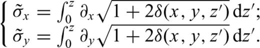
In this appendix we derive the first-order VTI wave equations in a stretched coordinate system. We follow the approach developed in Alkhalifah et al. (2001), but with a different change of variables and we apply it to the first-order wave equation.

The first-order formulation of eqs (2) is

(A1)

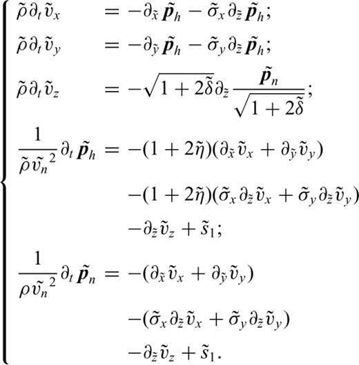
where and v_x, v_y and v_z are the components of the particle velocity.

With the change of variables in the stretched coordinate system, we replace

with

The wave equation becomes

(A2)

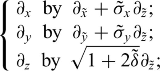
Neglecting the spatial derivatives of , we have and . This is valid with a smooth δ field but this is not valid at discontinuity. Transforming then the first-order formulation to the second-order formulation by eliminating and gives the eq. (4).

Appendix B: Additional Numerical Tests

In this appendix, we numerically evaluate the role of lateral variations of the δ parameter on the diving waves. We assume an elliptic medium. The vertical velocity is constituted of a water layer with a velocity of 1500 m s⁻¹ between 0 and 100 m depth, followed by a velocity varying linearly with depth from 1500 m s⁻¹ at 100 m depth to 3000 m s⁻¹ at 5 km depth. Because absorbing boundary conditions are imposed on all edges of the domain, with a source in the water layer, the seismograms contain two main events: the direct wave travelling horizontally in the water, and the diving wave caused by the velocity gradient.

We consider two δ fields: in case 1, δ varies laterally from 0 to 0.4, Fig. B1(a); in case 2, δ has a large lateral discontinuity from 0 to 0.3, Fig. B1(c). The corresponding stretched NMO velocities are displayed in Figs B1(b) and (d).

Figure B1

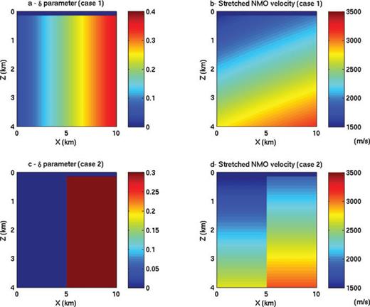
The δ parameter and stretched NMO velocities for the two numerical cases.

Open in new tabDownload slide

We generate for both cases a seismogram with the elliptic wave equation using the NMO velocity and the δ parameter and a seismogram with the isotropic wave equation using the stretched NMO velocity. The acquisition is a classic streamer acquisition with 9.5 km offset. The graphical comparisons of these seismograms are plotted in Fig. B2. With the laterally varying δ parameter the two seismograms are very similar. This confirms that the lateral derivatives of δ can be neglected in the change of variables described eq. (3) with a smooth δ field. With the laterally discontinuous δ parameter, the two seismograms are in phase, however the amplitudes differ especially near the discontinuity. This was expected, because the lateral derivatives of δ cannot be neglected close to a discontinuity.

Figure B2

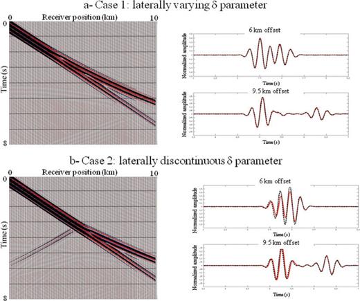
Comparison between seismograms computed with the elliptic wave equation and with the isotropic wave equation in a stretched coordinate system depending on δ. On the right-hand graphs, the seismograms computed with the elliptic wave equations are plotted in the background in red and blue, and the seismograms computed with the isotropic wave equation in black wiggles. The two seismograms are in phase when the blue loops match the black wiggles. On the left-hand graphs, the red traces correspond to the seismograms computed with the elliptic wave equation and the dashed black traces to the ones computed with the isotropic wave equation.

Open in new tabDownload slide

These examples illustrate the validity of the change of variables when neglecting δ derivatives, and thereby the relevance of the proposed parametrization of the FWI with NMO velocity and η (or horizontal velocity).

Appendix C: Time-Domain Formulation of the Acoustic VTI FWI

In this appendix, we derive the adjoint-state (backward) equations that need to be solved to compute the gradient with the adjoint-state technique. Following the approach described in Plessix (2006), we build an augmented functional of J by introducing one adjoint state per equation lines of the system (2) plus the equation that defines the synthetics

(C1)

The adjoint states are μ, λ_h and α_n. λ_h and λ_h are also called backpropagated fields.

The adjoint-state equations are obtained by equating to zero the derivatives of ℒ with respect to the state variables c, p_h and p_n. This gives after replacing μ by its value

(C2)

with the final conditions at T_max, the maximum recording time,

and the data residual

In practice, these equations are solved with initial conditions by time reversing the source terms, mainly the data residual r. The gradients with respect to v_n and η at a subsurface point x are (without taking into account the regularization term)

(C3)

(The summation over the source positions is implicitly contained in the scalar products.)

The first equation is equivalent, for the VTI case, to the equation developed by Lailly (1983) for the isotropic case. This can be seen as an imaging principle for VTI migration. From a kinematic point of view, we could a priori use only one of the terms of the gradient as imaging principle. This would avoid the storage of the two incident fields, p_n and p_h. We could even compute the back-propagated fields, λ_n and λ_h, with the state system (2) as it is done with the isotropic case. This however creates amplitude
 errors.

To analyse the amplitude behaviour, it is quite relevant to look at the approach proposed by Zhou et al. (2006), where a correction term to the acoustic isotropic wave equation is introduced. Following the idea described by Zhou et al. (2006), we define

(C4)

and the system (2) becomes

(C5)

with the initial conditions

If η is different from 0, we can divide the second equation by 2η and obtain a self-adjoint formulation. With this formulation, assuming the sources and receivers in an isotropic part of the medium, we define the synthetics by c=Sp. The two adjoint states, λ_p and λ_q, satisfy

(C6)

with the final conditions

With α₂= 1 and α₁= 0 and λ_n and λ_h defined by the system (C2), we have

(C7)

The gradient is given at a subsurface point x by

(C8)

Assuming η≠ 0, we define

The adjoint-state system (C6) written with and , is identical to the state system (C5). In fact, and are the adjoint states associated with the self-adjoint formulation obtained by dividing the second equation in system (C5) by 2η. If we now define and by

(C9)

we have

The gradient with respect to v_n is

(C10)

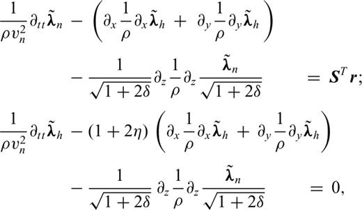
This formula should be used when the backpropagated fields are computed with the state system (2) and not the system (C2). It shows that cross-correlating only p_n with creates an error equal to in the gradient. This term is non-zero only with non-zero η. Indeed, with η= 0, p_h−p_n = 0 and has a finite value.

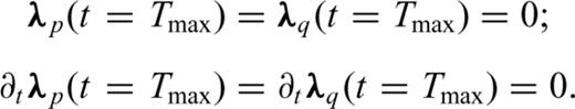
Appendix D: Source Estimation and FWI

The source estimation can be included in the FWI algorithm. In a first approach (Pratt 1999; Ravaut et al. 2004), the source wavelet becomes an unknown of the problem, namely is a model parameter. The misfit functional is now defined by

(D1)

with w the source wavelet parameters and f_c the misfit functional. For simplicity, we ignore the regularization term and consider ρ and δ fixed.

In the frequency domain, the wave-equation system, at a given angular frequency, can be written in a matrix form

(D2)

Here the subscript s indicates the source dependency, A is the wave operator, δ_s is a delta function source wavelet and S a sampling operator.

The misfit functional is

(D3)

Using the adjoint-state technique to derive the gradient (Plessix 2006), we build the augmented functional ℒ

(D4)

The adjoint-state equations are obtained by zeroing the derivatives with respect to the state variables p and c

(D5)

And the derivatives of the misfit functional are

(D6)

This approach imposes to estimate the source wavelet with the same misfit functional as the one used for the Earth parameters. For example, let us consider the misfit functional

(D7)

with W_d a real symmetric matrix.

The first equation of system (D5) gives

(D8)

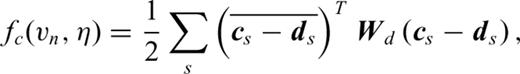
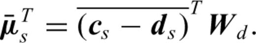
By replacing in the derivative with respect to w_s, in the first equation of system (D6), we obtain after equating this derivative to zero

(D9)

Defining u_s=Sp_s and since c_s=w_su_s[second equation of system (D2)], the source wavelet estimation is given by

(D10)

In a second approach, we estimate the source with a given formula. The state equations are now

(D11)

With this formulation, w_s is found with the state equation h_w=0 and is now a state variable. Here, w is not a model parameter and the misfit functional is

(D12)

The augmented functional becomes

(D14)

This second approach is more complicated to implement, however it gives more freedom in the source estimation. For instance, with the misfit functional used previously

(D15)

we can estimate the source by minimizing

(D16)

with W_w a real symmetric matrix.

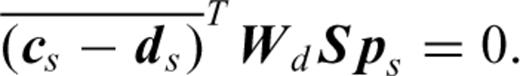
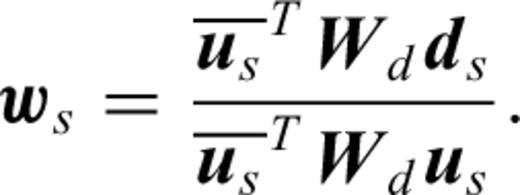
We could use such an approach when we focus the FWI on the long offsets with W_d and focus the source estimation on the short offset with W_w.

Zeroing the derivatives of f_w with respect to w gives

(D17)

We note that

is equal to 0 only when W_d=W}_w. In this case, the two approaches are equivalent. However, if , and the source terms of the backpropagated field, , are different in the two
 approaches.

References