Finite difference synthesis of infrasound propagation through a windy, viscous atmosphere: application to a bolide explosion detected by seismic networks

Summary

1 Introduction

The study of infrasound—subaudible acoustic energy—has undergone enormous advances since the first reports of barometric fluctuations observed worldwide after the eruption of Krakatoa (see Evers & Haak 2010 for a review). Early advances in infrasound studies were motivated by the utility of low-frequency sounds for estimating gradients in wind and temperatures at high altitudes (e.g. Gutenberg 1939). After World War II, progress in infrasound was driven by the need to monitor the Earth and atmosphere for clandestine nuclear tests. Ultimately, this led to the construction of a global network of infrasound stations (Christie & Campus 2010), which is being deployed as one component of the International Monitoring System (IMS) and is designed to monitor nuclear explosions. Many natural sources are also detected at this network so that its development has rekindled interest in the use of infrasound to examine a wide variety of atmospheric and geophysical phenomena, including ocean swell (Garcés et al. 2003; Hetzer et al. 2010), ocean surf (Arrowsmith & Hedlin 2005), tsunamis (Le Pichon et al. 2005a), earthquakes (Le Pichon et al. 2006; Mutschlecner & Whitaker 2005), volcanoes (Matoza et al. 2006; Fee & Garcés 2007; Matoza et al. 2009) and meteors (Revelle et al. 2004; Edwards 2010).

Although the global IMS stations are augmented by several dozens of regional arrays worldwide, the infrasound network remains sparse compared to typical seismic networks. To compensate for gaps in spatial coverage, a number of infrasound studies have used presumed air-to-ground coupled arrivals recorded on seismometers to examine the infrasound wavefield in detail. Acoustic arrivals from the explosion of the 2005 December Buncefield oil depot, in the United Kingdom, were recorded at infrasound arrays and seismometers across central Europe. Atmospheric ray tracing confirmed that arrivals were associated with ducting through the troposphere, stratosphere and the thermosphere (Ottemöller & Evers 2008; Ceranna et al. 2009). Tropospheric and stratospheric arrivals generated by the descent of the shuttle Atlantis over southern California in 2007 June were detected at over 100 seismometers associated with the transportable USArray network and other regional networks (de Groot-Hedlin et al. 2008). More recently, a bolide explosion in northeastern Oregon in 2008 February generated tropospheric, stratospheric and thermospheric arrivals that were detected at four infrasound arrays in Canada and the United States and by 500 seismic stations in the US Pacific Northwest (Hedlin et al. 2010).

The efficacy of infrasound for remotely sensing natural and anthropogenic hazards stems from the excellent transmission characteristics of low-frequency acoustic signals through the atmosphere. Both tropospherically and stratospherically ducted infrasound undergo minimal absorption within the atmosphere; the former depend mainly on diurnal sound and wind speed variations, while the latter depend on seasonally varying stratospheric winds. As a result, detection rates of stratospherically ducted infrasound vary seasonally, which has implications for the detection thresholds of the IMS infrasound network (Le Pichon et al. 2009).

Thermospheric signals, which propagate between the ground and lower thermosphere, may be the only infrasound arrivals. They are predicted in every direction, for all seasons, due to the steep sound speed gradients at altitudes over 90 km. However, infrasound signals along this path are thought to be highly attenuated due to enhanced absorption within the thin air of the upper atmosphere so that only very large infrasound sources generate detectable thermospherically refracted arrivals. Thermospheric signals generated by large volcanic eruptions (Evers and Haak 2005; Le Pichon et al. 2005b; Le Pichon et al. 2005c) and the Buncefield vapour cloud explosion (Ceranna et al. 2009) have been detected at infrasound arrays. The Buncefield explosion (Ottemöller & Evers 2008; Ceranna et al. 2009) and a bolide terminal burst (Hedlin et al. 2010) generated thermospheric signals that were detected as air-to-ground coupled arrivals at seismic stations.

A combined analysis of stratospheric and thermospheric arrivals generated by a single large source may provide tighter constraints on source characteristics of very large explosions (Whitaker & Mutschlecner 2008). However, a problem with relying on detections of thermospheric arrivals is that wind and sound speeds above about 50 km are poorly constrained. The current standard in atmospheric specifications is to fuse operational weather analysis—which is updated several times daily—within the troposphere and stratosphere, with empirical climatologies above (Picone et al. 2002; Drob et al. 2003). A further difficulty is that acoustic absorption is also poorly constrained at high altitudes. Attenuation values have been predicted for altitudes up to 160 km, but estimates above 90 km are imprecise due to uncertainties about atmospheric composition (Sutherland & Bass 2004).

The development of more precise estimates of thermospheric attenuation has been hampered both by the low density of infrasound stations, and the lack of waveform synthesis methods that handle infrasound attenuation. The utility of USArray seismic stations for recording infrasound signals has lessened the first problem. However, numerical methods that include the effects of both wind and attenuation are needed in modelling infrasound propagation at altitudes over 50 km. In previous efforts, the effect of wind has been introduced into a parabolic equation (PE) modelling algorithm (Lingevitch et al. 2002) and finite-difference time-domain (FDTD) methods (Van Renterghem and D. Botteldoren 2003; Ostashev et al. 2005). In frequency-domain modelling methods, like PE or fast field program (FFP) methods (e.g. Jensen et al. 1994), attenuation is introduced by adding a small, non-physical, imaginary term to the acoustic velocity. An acoustic viscosity term was introduced directly into the governing equations of an FDTD algorithm (de Groot-Hedlin 2008). This method yields attenuation values that increase with the square of the frequency, in agreement with theory (Sutherland & Bass 2004).

In this paper, we introduce an FDTD algorithm that includes both wind and attenuation and apply it to explain infrasound arrivals, including thermospheric arrivals, generated by a terminal bolide explosion that occurred over northeastern Oregon on 2008 February (Hedlin et al. 2010; Walker et al. 2010). Air-to-ground coupled arrivals were recorded at 500 broad-band seismic stations of the USArray and regional networks including the Wallowa Flexible Array network and the High Lava Plains Seismic Experiment, which were deployed to investigate crustal and upper-mantle structure of the region. In Hedlin et al. (2010), 3-D atmospheric ray tracing was used to identify arrivals as tropospherically, stratospherically or thermospherically ducted; the results confirmed that late arrivals to the southwest of the bolide explosion were associated with thermospheric returns. The source time and location of the terminal burst were determined by a combination of video observations, infrasound arrays, backprojecting USArray seismic waveform envelopes and modelling the timing of direct arrivals at 13 seismic stations located within a 87 km radius of the burst (Walker et al. 2010). The high signal-to-noise ratios of the thermospheric arrival at many receivers, together with accurate source parameter estimates, allow us to test our newly developed FDTD infrasound propagation algorithm on real data. We show that our synthetic modelling results—based on current knowledge of atmospheric sound speeds, wind speeds and attenuation—agree with observed infrasound signals to first order.

This paper is structured as follows. The linearized equations governing acoustic wave propagation in a windy, absorptive medium are derived in the next section. A FDTD approach to solving these equations in a stratified, range-independent medium is presented in the Section 3. Section 4 shows the application of the method to data from the bolide. In Section 5 we discuss differences between the observed data and synthesized results, with implications for acoustic propagation and absorption in the thermosphere. Section 6 gives concluding remarks.

2 Linear Infrasound Propagation in a Windy, Absorptive Medium

The energy dissipation that occurs during any fluid motion, including fluctuations associated with acoustic propagation, affects that motion. At infrasonic frequencies and altitudes over 60 km, internal friction (viscosity) is the dominant absorption mechanism; at lower altitudes, infrasound absorption is dominated by molecular vibration losses, which involves the excitation of gas molecules comprising the atmosphere (Sutherland & Bass 2004). However, the latter absorption mechanism leads to losses of less than about 10⁻⁵ dB km⁻¹ at infrasonic frequencies and thus is neglected here. Therefore, in this paper we consider only absorption losses caused by atmospheric viscosity. Although the energy dissipation is irreversible, we also apply the standard assumption of isentropy, that is, that entropy of the wave motion remains unchanged. More precisely, some dissipation of energy occurs in the presence of viscosity, but it can be shown that this is only a second-order effect, and may therefore be neglected for linear propagation modelling.

In this section, we derive coupled equations for infrasound propagation through a windy, viscous atmosphere. The equation for the acoustic pressure fluctuations p

1

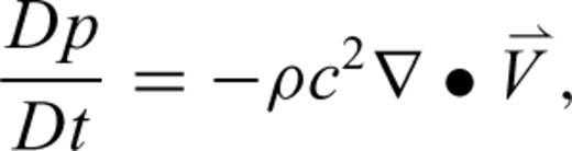
derived by combining the equations of state and conservation of mass, relates the total particle velocity, , density, ρ and sound speed c to the advective derivative of the pressure, where the advective derivative is given by 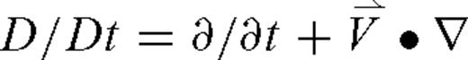. The Navier–Stokes equation for a compressible viscous fluid gives the acoustic particle velocity

2

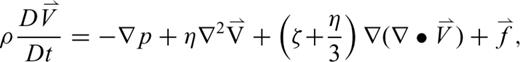
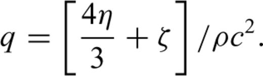
(eq. 15.6 of Landau & Lifshitz 1959) where is an external source acting upon the medium, η is called the viscosity coefficient and ζ is variously called the second, volume or bulk viscosity. The term denotes the vector [∇²V_x,∇²V_y,∇²V_z]. Both viscosity coefficients vary only slightly in the atmosphere; in fact, this was assumed in the derivation of eq. (2) (Landau & Lifshitz 1959). The value of η for air is approximately 1.8 × 10⁻⁵ kg m⁻¹ s⁻¹ and the bulk viscosity ζ is usually of the same order of magnitude (Landau & Lifshitz 1959); Pierce (1981) gives ζ= 0.6η. However, the bulk viscosity is often omitted (e.g. Gill 1982; de Groot-Hedlin 2008).

The pressure, density and velocity fields fluctuate due to the propagation of a sound wave within a medium. The pressure, density and velocity fields are expressed as the sums of their ambient values and perturbations caused by the passage of a sound wave.

3

where the ambient pressure and density values are denoted by the o subscript, and s denotes perturbations caused by passage of a sound wave. Here denotes the wind speed and is the acoustic particle velocity. Waveforms are derived by computing the pressure fluctuations as a function of time.

Eqs (3) are inserted into eqs (1) and (2) to derive a set of linear partial differential equations for the pressure and particle velocities. It is assumed that the background field is in stable equilibrium, that is, that eqs (1) and (2) are satisfied in the absence of a sound wave, so that zero-order terms cancel. Only linear terms in the pressure, density and particle velocities are retained, under the assumption that pressure and density fluctuations due to the passage of a sound wave are only a small fraction of the ambient values, and that the particle velocities are small compared to the sound speed. We also assume that ∇ρ_o=∇p_o= 0 which is valid at typical infrasound frequencies where buoyancy waves are insignificant, that is, we consider only frequencies greater than 3 mHz (Lingevitch et al. 1999). If it is assumed that the divergence in the wind speed is negligible (i.e. ), as in (Ostashev et al. 2005), eq. (1) becomes

4

Over large scales, it is assumed that vertical component of wind is negligible compared to the horizontal components and so is set to zero in the G2S models often used for computation of infrasound propagation (Drob et al. 2003). Therefore in the following, we assume that winds are horizontal and that wind gradients are only vertical. Then eq. (2) yields

5

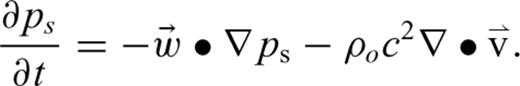
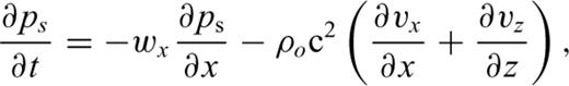
For horizontal winds that vary with altitude, . Note that terms involving fluctuations in the atmospheric density ρ_s drop out of the equations when gravity is neglected. Eqs (4) and (5) are the governing equations for infrasound propagation in a viscous, windy atmosphere; a numerical method of infrasound waveform synthesis for a general model with varying densities, and sound and wind speeds is described in the next section.

In the remainder of this section, we derive an analytic expression for the pressure wavefield for a highly simplified model in which the density and sound speed are uniform, and there is no wind. In this way, we demonstrate that the inclusion of the viscosity terms into the propagation equations leads to the attenuation and dispersion of the computed acoustic arrivals. In this case eqs (4) and (5) may be combined to yield a single analytic expression.

6

where

7

Eq. (6) describes a medium in which internal viscosity is the dominant absorption mechanism (Lighthill 1978).

We insert a trial plane wave solution of the form

8

into eq. (6) where ω is the circular frequency, is the vector distance and t is the time, to solve for the wavenumber . We obtain the complex-valued, squared wavenumber

9

The wavenumber is related to the frequency-dependent wave speed c_p and attenuation α through k(ω) =ω/c_p(ω) + i α (ω). We write k²(ω) in exponential notation as k² = |k²|e^iφ, where φ is the argument of k² to derive

10a

and

10b

Applying trigonometric half-angle formulae, it can be shown after some algebraic manipulation that the expression for the frequency-dependent sound speed is given by

11

and the expression for atmospheric attenuation is given by

12

Eqs (7), (11) and (12) imply that phase velocities and attenuation are dependent on the coefficients of attenuation, static sound speeds and atmospheric density. Throughout the infrasound range, that is, up to frequencies of 20 Hz, and at altitudes below 100 km, qω≪ 1, so the dispersion relation and attenuation may be approximated as

13

and

14

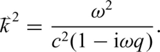
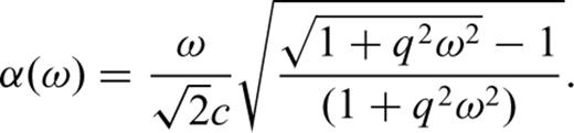
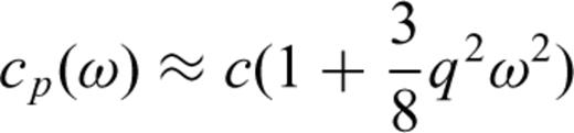
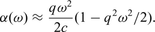
Eqs (13) and (14) indicate that both dispersion and attenuation are approximately proportional to the square of the frequency for qω≪ 1; eq. (7) implies that both values increase with decreasing density. Since the atmospheric density decreases exponentially in the atmosphere, high frequencies are increasingly attenuated and dispersed in the Earth's upper atmosphere. Consequently, sound waves refracted within the thermosphere should be dispersed and have less power at higher frequencies than those refracted at lower altitudes.

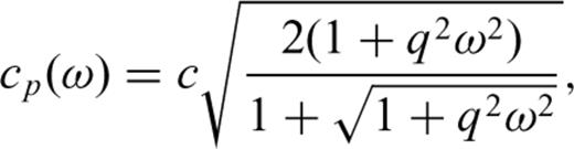
Atmospheric sound speeds and densities vary over scale lengths much longer than the infrasound wavelength, thus eqs (11) and (12) may be used to derive infrasound attenuation and phase speeds for a stratified atmosphere with slowly changing sound speed and density variations. Fig. 1 shows the attenuation and dispersion derived from eqs (11) and (12) for a sound speed profile in northeastern Oregon on the morning of 2008 February 19. This profile is relevant to a bolide explosion that will be examined in greater detail in Section 4. The atmospheric density profile, also shown in Fig. 1, is derived using the hydrostatic equation for pressure gradients combined with the ideal gas law relating density and temperature to pressure, and c²=kRT, relating sound speed and temperature T (k= 1.4 is the ratio of specific heats, and R= 287.04 J kg⁻¹ K⁻¹ is the gas constant for dry air).

Figure 1

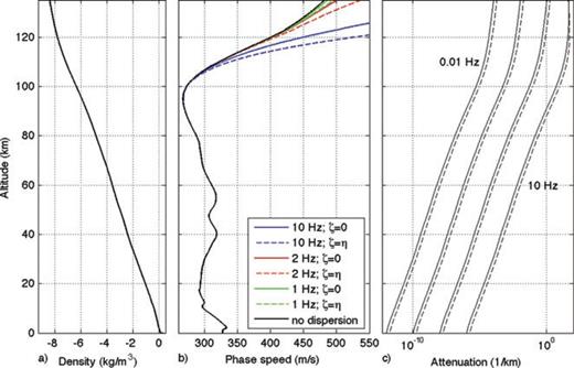
(a) Atmospheric density profile corresponding to the static sound speed profile in b. (b) Static sound speed profile (black) and phase speed profiles computed for several infrasound frequencies. Phase speeds have been computed for ζ=η= 1.8 × 10⁻⁵ kg m⁻¹ s⁻¹, and for ζ= 0. (c) Attenuation coefficients α(ω) computed at frequencies of 0.01, 0.1, 1 and 10 Hz, for ζ=η= 1.8 × 10⁻⁵ kg m⁻¹ s⁻1 (dashed lines), and for ζ= 0 (solid lines).

Open in new tabDownload slide

Fig. 1 shows that there is significant dispersion at the upper end of the infrasound frequency range. Phase speeds are significantly higher than the static sound speeds at an altitude of 120 km and a frequency of 10 Hz. At a result, acoustic energy at this frequency would be mostly refracted downwards and little energy could penetrate to higher altitudes. At lower frequencies, infrasound energy can propagate to higher altitudes but undergoes significant absorption as shown in Fig. 1(c). Below 1 Hz, phase speeds are nearly identical to static sound speeds at altitudes below 125 km so that dispersion would be negligible. An alternative method of deriving the velocity dispersion (Bass et al. 2007) yields similar dispersion values up to 120 km at infrasound frequencies; at higher altitudes, their results suggest greater dispersion.

The attenuation values shown in Fig. 1(c) are similar to those derived from the formulae in Sutherland & Bass (2004) at altitudes above 60 km, reflecting the fact that viscosity is the dominant loss mechanism at high altitudes. The attenuation values at lower altitudes are smaller, reflecting the fact that other loss mechanisms that dominate at lower altitude are neglected here. However, as previously stated these losses are negligible at infrasound frequencies.

3 Numerical Implementation

3.1 The FDTD approach

Eqs (4) and (5) form a complete set of coupled equations for the pressure and acoustic particle velocity, given ambient values for the atmospheric sound speeds, wind velocities and attenuation constants. These equations are amenable to solution by the FDTD approach, which is based on replacing the spatial and time derivatives in the governing equations by their difference approximations. The pressure and particle velocities may then be computed over a set of discrete nodes that comprise the spatial and temporal grids.

This method of solution is presented here for 2-D models, using a staggered spatial grid as shown in Fig. 2. In 2-D, the model is divided into a grid of cells of dimension Δx by Δz, each with a uniform density ρ₀ and static sound speed c. Pressure variables are sampled at the centre of each cell and the particle velocity components are sampled at points along the cell boundaries. The primary advantage of using the spatially staggered grid is that it provides centred spatial differences for many of the derivatives in the FDTD implementation, which are accurate to second order, rather than forward or backward differences, which are accurate only to first order. Higher order spatial or temporal finite-difference methods are available which would lead to equivalent accuracy with a coarser grid sampling than is used with the simple central difference operators applied here. However, the objective here is to demonstrate the applicability of the FDTD method for simulating infrasound propagation in a windy, absorptive medium.

Figure 2

The finite-difference model is decomposed into a set of discrete cells, indicated by the solid lines, each with uniform static sound speed c and ambient density ρ_o. The acoustic pressure and density perturbations are defined at the nodes at the centre of each cell, indicated by the filled circles. The horizontal particle velocity v_x (triangles pointing right) and vertical particle velocity variables v_z (triangles pointing up) nodes straddle the cell boundaries of the spatially staggered grid, shown in two dimensions.

Open in new tabDownload slide

Expanding the governing equations (Eqs 4 and 5) in a 2-D Cartesian coordinate system in terms of individual components yields the update equations for the pressure fluctuations.

15

and for particle velocities

16

17

The solution method may be simplified when there is no wind and only pressure values are sought. In that case, the and terms can be combined as in the particle velocity equations. This would yield slight inaccuracies in the particle velocities but the computed pressures would remain accurate because the action of the divergence operator in the pressure equation (eq. 4) on the attenuation terms yields . This would be justified if only the pressure were of interest rather than particle velocity.

Eqs (15)–(17) differ from those for a static atmosphere by the introduction of the advection terms involving w_x∂/∂x and the wind shear term v_z∂w_x/∂z in eq. (16). Several numerical implementations have been suggested for the computation of the FDTD equations for sound propagation in windy environments (Blumrich & Heinmann 2002; Van Renterghem & Botteldoren 2003; Ostashev et al. 2005). In particular, it is noted that inclusion of wind velocities in the first-order equations complicates the standard method of staggering the velocities and pressures in both space and time, since the advection terms in the update equations imply that the first-order derivatives in space and time are computed simultaneously, rather than serially as in the usual FDTD approach. Here, we use the FDTD method introduced by Ostashev et al. (2005) for computing acoustic waves advected through a windy atmosphere. They suggest the use of a ‘non-staggered leap-frog’ scheme, in which one forms centred temporal finite differences over two time steps, rather than the single time step in the staggered leap-frog approach (Yee 1966).

To explain the use of this FDTD scheme, we adopt the notation

18a

18b

and

18c

We assume a model that is temporally invariant and vertically stratified, so the wind, sound speed and ambient density are represented as w_n=w_x(nΔz), c_n=c(nΔz) and ρ_n=ρ_o(nΔz). Here, we have dropped the x subscript on the wind since only horizontal winds are considered. The s subscript on the pressure is dropped since there are no ambient pressure terms, and the 0 subscript on the density is dropped since there are no terms involving density fluctuations. Using this notation, the update equation for the pressure fluctuations becomes

19

This equation indicates that updating the pressure in time requires storing each pressure field variable over two time steps, rather than over a single time step as in the standard leap-frog approach. That is, the values of the particle velocities at the jth time point and the pressures at the jth and (j− 1)th time points are used to find the pressure at time j+ 1. The motivation for this is that we retain the accuracy of central differences in the temporal differencing operator, making the algorithm accurate for high Mach numbers. For the same reason the spatial finite differences in the advection term is taken over two gridpoints to provide centred spatial differences.

Similarly, the equation for the horizontal particle velocity becomes

20

and the equation for the vertical particle velocity is

21

where and are the horizontal and vertical forces, respectively, acting in the horizontal direction at location mΔx, nΔz. The term denotes the average particle velocity at the location of the node. As in Ostashev et al. (2005) it is derived from the average of the four closest vertical particle velocities surrounding the horizontal velocity (see Fig. 2). The term ρ_n+1/2 in eq. (21) denotes the average ambient density in the cells above and below the node for v_z.

The perfectly matched boundary layer method (Berenger 1994) is used to absorb waveforms at each boundary. Eqs (19)–(21) are used to march the solution out in time, and the time-dependent pressure fluctuations are saved at locations corresponding to receiver locations.

3.2 Numerical accuracy

Solutions derived using FDTD methods are inexact because the discretized equations (eqs 19–21) are approximations to the continuous differential equations that they replace (eqs 4 and 5). The magnitude of the errors depends on the sampling rates in both the spatial and temporal grids. The errors are manifested as numerical dispersion and spurious attenuation or growth; these non-physical artefacts are inherent to all FDTD techniques (e.g. Taflove & Hagness 2000). Note that numerical dispersion is an error introduced by discretizing the governing equations, and is distinct from the dispersion discussed in Section 2, which is a physical phenomenon.

We compute the numerical dispersion for the coupled equations by considering a very simple homogeneous medium with uniform density, sound speed, wind speed and viscosity. We know that the analytic solution is a wave equation of the form . Thus we may postulate solutions of the form

22a

22b

and

22c

where and are the finite-difference approximations to the exact horizontal and vertical wavenumbers. The numerical approximations to the wavenumber differ from the true value of by an amount that depends on the node spacing, the temporal resolution, as well as the frequency, the sound and wind speeds and the direction of propagation.

Substituting eq. (22a) into the finite difference operator for ∂p/∂t in eq. (19) leads to

23

using Euler's formula. We adopt the following notation:

24

These values all approach 1 in the limit of small Δx, Δz and Δt. Applying the substitutions eqs (22) to eqs (19)–(21) leads to

25

26

27

The numerical dispersion relation is derived by combining eqs (25)–(27) to arrive at

28

for a homogeneous, absorptive medium with uniform wind. Finally, we use square cells within the model grid, so that Δx=Δz=Δ, so and 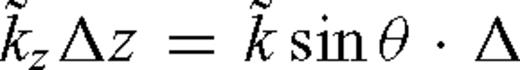, where θ is the propagation angle with respect to the x-axis. Eq. (28) then indicates that the numerical errors are a function of the propagation direction as well as the temporal and spatial sampling rates.

The grid and time sampling rates in an FDTD simulation depend on the highest frequencies used for propagation modelling. However, the finite-difference propagation equations do not lead to a closed form expression for a stability limit on Δt when winds and attenuation are included. Instead we rely on modifying the Courant stability limit derived for a time-staggered algorithm for a viscosity-free, windless model (Δt=Δ/c) for a guideline in choosing the time sampling rate. Our ‘non-staggered leap-frog’ approach in which centred differences are formed over two time steps requires halving the sampling rate, and the inclusion of wind suggests that Δt be further reduced to account for the change in wavelength due to advection. This suggests a maximum time sampling rate of Δt=Δ/[2(c+w)]. For example, we consider a model with sound speed c= 350 m s⁻¹ and a wind speed of +50 m s⁻¹ in the +x-direction, and a source with upper frequency 0.5 Hz. A node spacing of 60 m results in sampling the waveform at 10 points in the direction of negative wind velocity at the upper end of the source bandwidth. The corresponding maximum time sampling rate would be 0.075 s; for greater accuracy, we chose a time discretization of 0.0375 s. We use the secant method to solve eq. (28) for the values of as a function of propagation angle, where the angle is defined positive anticlockwise with respect to the +x-axis.

Fig. 3(a) shows the normalized numerical sound speed as a function of propagation angle at the maximum source frequency for models with η=ζ= 1.8 × 10⁻⁵ kg m⁻¹ s⁻¹ at a density ρ_o= 1 × 10⁻⁷ kg m⁻³, equivalent to an altitude of about 110 km. These values, shown as dots, are superimposed on the values for numerical errors computed without attenuation. It is notable that the numerical sound speed is minimally affected by the attenuation. The figure indicates that numerical inaccuracies is a maximum for propagation directly upwards (or downwards) however, the total difference is less than 2 per cent for the given discretization values. Fig. 3(b) shows the normalized attenuation factors as a function of propagation angle, again indicating that the FDTD technique is the least accurate in a direction perpendicular to the wind, with the attenuation overestimated by as much as 6 per cent.

Figure 3

Numerical errors in the FDTD algorithm as a function of propagation angle for a model with c = 350 m s⁻¹, w= 50 m s⁻¹ in the +x-direction, at a frequency of 0.5 Hz. Propagation angle is anticlockwise with respect to the +x-axis. (a) Variation of the normalized sound speed ratio . The solid line are the values computed for a model with no attenuation. The dots indicate values computed for η=ζ= 1.8 × 10⁻⁵ kg m⁻¹ s⁻¹ at a density ρ_o= 1 × 10⁻⁷ kg m⁻³. (b) Variation in attenuation ratios for a model with attenuation as in (a).

Open in new tabDownload slide

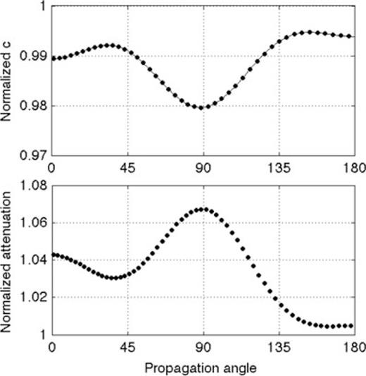
The results of Fig. 3 only show the numerical errors introduced by the FDTD method at the very highest frequencies considered in the propagation; accuracy is greater at the lower frequencies. Fig. 4 shows the normalized numerical sound speeds and dispersion values as a function of frequency for the same parameters and discretizations considered above, but this time for frequencies from 0 Hz to 0.5 Hz. The normalized sound speed and attenuation values are computed for a propagation angle of 0°, that is, for propagation in the +x-direction. As indicated, the numerical errors increase as a function of frequency, but errors in the normalized sound speed remain small, on the order of 1 per cent, up to the maximum source frequency of 0.5 Hz considered for this example. Errors in attenuation also increase as a function of frequency and reach 6 per cent at the upper source frequency. However, we consider this acceptable given that atmospheric attenuation values are not known precisely. Note that, since attenuation increases with increasing frequency, this formulation is more stable than that of de Groot-Hedlin (2008), where attenuation decreased with increasing frequency.

Figure 4

Numerical errors in the FDTD algorithm as a function of frequency for a model as in Fig. 3, computed at a propagation angle of 0°. (a) Variation of the normalized sound speed ratio . The solid line are the values computed for a model with no attenuation. The dots indicate values computed for η=ζ= 1.8 × 10⁻⁵ kg m⁻¹ s⁻¹ at a density ρ_o= 1 × 10⁻⁷ kg m⁻³. (b) Variation in attenuation ratios for a model with attenuation as in (a).

Open in new tabDownload slide

4 Application to Bolide

4.1 Bolide explosion

A bolide was observed before dawn on 2008 February 19 above northwestern states in the continental United States and western provinces of Canada. The source time and location of this event were determined with unusually high precision using data from seismic networks, global infrasound arrays and video observations (Walker et al. 2010). Specifically, acoustic-to-seismic coupled signals from the event registered clearly at 700 seismic stations in regional networks and in the USArray Transportable Array. The close agreement between the seismic location and time of the event and the video location and time of the terminal burst indicates that the seismic signals were not due to sound shed from the hypersonic object as it passed through the atmosphere but from its terminal burst.

Because the location and time of the bolide explosion could be determined so precisely using the acoustic-to-seismic coupled signals, and because the source was impulsive, Hedlin et al. (2010) used the event to model the infrasound propagation out to a range of 500 km. Specifically, they picked the rise times for the different phases, an approach that is not impacted significantly by complications that arise from site-to-site variations in acoustic-to-seismic transmission characteristics. Atmospheric ray tracing was performed to predict traveltimes in a fully range-dependent, 3-D environment. The wind and sound speeds were derived from European Centre for Medium-Range Weather Forecasts (ECMWF) analysis products (Persson & Grazzini 2007) up to an altitude of 75 km and the HWM07/MSISE-00 empirical climatologies (Picone et al. 2002; Drob et al. 2008) above 75 km. They found that most arrivals were either tropospheric or stratospheric in origin. However, a cluster of late arrivals to the southwest of the bolide explosion was associated with refraction in the thermosphere.

In this section, we examine arrivals along a single azimuth and perform ray tracing to identify expected travel paths, traveltimes and expected frequency content for simplified 1-D sound and wind speed profiles. We then use the FDTD method described above to synthesize a cluster of late arrivals at stations to the southwest of the source, at ranges over 250 km, identified by ray tracing as being associated with refraction in the lower thermosphere (Hedlin et al. 2010).

4.2 Preliminary modelling using ray tracing

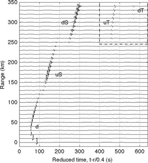
For the time period of interest to this study, noise levels at USArray seismic stations peaked at about 0.2 Hz, roughly the peak of the microbarometric spectrum; at this frequency, noise levels were approximately four orders of magnitude greater than between 2 and 8 Hz. Infrasound signals were not observed at frequencies below 1 Hz, almost certainly because noise levels were too high. Fig. 5 shows 2–8 Hz bandpassed waveforms recorded at seismic stations along an azimuth of 210^o, for ranges up to nearly 350 km from the source. A reducing velocity of 400 m s⁻¹ was used to allow us to display the signals more clearly. To illustrate infrasound propagation along this azimuth, ray paths were recomputed for simplified atmospheric sound and wind profiles using a tau-p method developed for an advected medium (Garcés et al. 1998). We used identical wind and sound speed profiles for the ray and FDTD computations to provide a direct comparison of results. Since deviation of the infrasound travel path out of the source–receiver plane cannot be considered for the 2-D FDTD computations, we neglected cross-wind components in our model. Furthermore, examination of the ECMWF analysis products and HWM07/MSISE-00 empirical climatologies for this event indicated that there was little variation in wind and sound speeds along path to a range of 350 km from the source; the mean along path variations at each altitude were 0.6 m s⁻¹ in sound speed and 1.8 m s⁻¹ in wind speed. Consequently, atmospheric wind and sound speeds were represented by range-independent values that were derived by averaging the sound and wind profiles along this azimuth. The average sound speed profile was shown in Fig. 1(b) as the static sound speed profile; the average wind speed profile along the path is shown in Fig. 6.

Figure 5

Seismic velocity responses, bandpassed from 2 to 8 Hz, along a profile from 210° with respect to north. Ranges are with respect to the source location. The timescale has been reduced by 400 m s⁻¹. The traces have been scaled such that each waveform has the same peak amplitude. Arrivals are labelled using the nomenclature of Hedlin et al. (2010).

Open in new tabDownload slide

Figure 6

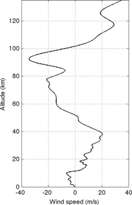
Average wind speed profile for 1400 UT, 2008 February 19, along a 350 km path at an azimuth of 210° from north, beginning at the location of the bolide explosion. Static sound speeds were shown in Fig. 1(b).

Open in new tabDownload slide

Fig. 7(a) shows computed ray paths for propagation along this azimuth. For these computations, the Earth's surface was represented by a rigid, flat boundary at an elevation of 1450 m, the average elevation above sea level at this azimuth. Rays were calculated up to a maximum altitude of 123 km, and only rays that reach the ground are shown. Rays turning above this altitude were excluded from this study due to the predicted high attenuation. Ray tracing shows that the first arrivals at each station either propagated directly downwards from the source (branch d, using the nomenclature of Hedlin et al. 2010), or were then tropospherically ducted (dWn; predicted at ranges beyond 100 km). Beyond about 150 km, these arrivals merge with a branch of acoustic energy that initially propagated upwards from the terminal burst and was then refracted back to the Earth within the stratosphere (branch uS) with additional arrivals at greater ranges predicted due to ducting in the troposphere (branch uSWn). The second arrivals, observed at distances starting about 250 km, result from acoustic energy that is stratospherically ducted after first propagating down from the source and reflecting from the Earth's surface (branch dS). The third set of arrivals, beyond 225 km from the source and about 4 min after the first arrivals, are thermospherically ducted after being directed up from the source (uT). The final set of arrivals in the ray diagram is identified with infrasound energy that is thermospherically ducted after first propagating down from the source and reflecting from the Earth's surface (branch dT). Note that the arrival pattern shown in Fig. 7(b) is a reasonably close match to the real data (Fig. 5), with the exception of the final branch dT, which is not observed in the waveform data.

Figure 7

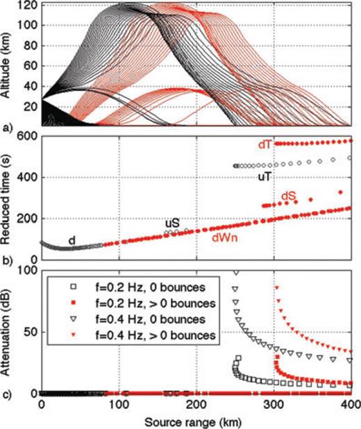
(a) Ray diagram, showing rays that reach the ground. Black lines indicate rays that have not undergone reflection at the surface. Rays that have undergone at least one bounce are shown in red. A flat ground surface has been used to compute ray paths, so that rays do not steepen or become shallower as they bounce along the surface. (b) Corresponding arrival times, reduced by 400 m s⁻¹. Arrivals are labelled using the nomenclature of Hedlin et al. (2010). (c) Corresponding attenuation values, at f= 0.2 Hz and f= 0.4 Hz, computed for a viscosity coefficient of η= 1.8 × 10⁻⁵ kg m⁻¹ s⁻¹ and bulk viscosity ζ= 0.6 η. Significant attenuation is predicted only for thermospheric rays.

Open in new tabDownload slide

We use ray tracing to obtain a first-order estimate of the attenuation for a given ray path. Given the computed ray path, and the equation for the attenuation due to viscosity as a function of density, sound speed and frequency (eq. 12, and see Fig. 1c), approximate attenuation values for each path can be computed by integrating the absorption values along segments of each ray path. The total attenuation along each ray path is shown in Fig. 7(c) for 0.2 Hz and 0.4 Hz. As indicated, infrasound propagating in the troposphere and stratosphere undergoes negligible attenuation at these frequencies, while thermospheric returns undergo significant absorption. Rays that propagate higher than 120 km altitude are even more highly attenuated. Note that attenuation estimates based on ray results do not yield relative amplitudes between tropospheric, stratospheric and thermospheric returns since these results do not take relative ray densities into account. Fig. 1 indicates that there is no significant physical dispersion at these frequencies.

4.3 FDTD simulation of low-frequency infrasound propagation

The ray path analysis suggests that thermospheric returns undergo substantial attenuation at frequencies above at least 0.2 Hz; as indicated in Fig. 7(c), infrasound undergoes about 6 dB attenuation at 0.2 Hz, that is, the amplitudes are halved; at 0.4 Hz, the attenuation is about 30 dB and amplitudes are reduced by approximately a factor of 30. Thus, we used a source term with a maximum frequency of 0.45 Hz in our FDTD simulation of low-frequency infrasound propagation from the bolide terminal burst to compare the differences in predicted absorption between tropospheric/stratospheric and thermospheric paths. We do not consider higher frequencies because of limited computational resources. The bolide explosion is represented temporally as a Gaussian pulse and spatially as a point at 27 km altitude; the source is modelled as an external force added to the particle velocity terms, as in eq. (2).

The waveforms in Fig. 5 show the vertical seismic velocity responses, so in the FDTD simulation we model the vertical particle velocities v_z, which were sampled every 10 km along the ground to a range of 340 km. Unless otherwise stated, the ground was modelled as a flat boundary at an elevation of 1.45 km, equal to the average elevation along a transect 210° from the bolide terminal burst. The top of the model was set to 123 km altitude. Given the sound and wind speed profiles displayed in Figs 1(b) and 6, and the maximum source frequency of 0.45 Hz, a node spacing of 50 m was chosen. For the lowest sound and wind speeds (and upper source frequency), this yields a node spacing of 11 nodes per wavelength.

The FDTD synthesis was run four times: (1) with attenuation using a viscosity coefficient of η= 1.8 × 10⁻⁵ kg m⁻¹ s⁻¹ and bulk viscosity ζ= 0.6 η, (2) with no attenuation, (3) with the Earth's surface lowered to an elevation of 0 km and (4) with realistic topography included, where elevations were taken from the ETOPO1 global relief model (Amante & Eakins 2009). For the runs where attenuation was included, the time sampling rate was set to 0.0287 s. For the run where attenuation was neglected, the time sampling rate was set to 0.0382 s.

Fig. 8 shows the result of the FDTD synthesis run with attenuation, with viscosity η= 1.8 × 10⁻⁵ kg m⁻¹s⁻¹ and bulk viscosity ζ= 0.6 η. For comparison, Fig. 9 shows the equivalent results for the FDTD computations without attenuation. Both FDTD simulations show that the dS arrivals, those that are refracted in the stratosphere after reflection at the Earth's surface appear at ranges of nearly 250 km from the source, in agreement with the data. Furthermore, the first thermospheric arrivals appear at approximately the same range, and at times that provide a close fit to the data. However, the main difference between the waveforms of Figs 8 and 9 is in the late arrivals associated with refraction in the thermosphere. The amplitudes of the late arrivals in Fig. 8, computed with non-zero viscosity, are lower than those of Fig. 9; the higher frequencies have been preferentially attenuated in Fig. 8 as expected.

Figure 8

FDTD synthesized v_z waveforms for stations at 10 km intervals from a source at 27 km altitude. This shows the results of simulation 1: the FDTD algorithm was run with a viscosity coefficient of η= 1.8 × 10⁻⁵ kg m⁻¹ s⁻¹ and bulk viscosity ζ= 0.6 η, and the ground was modelled as a flat surface at an elevation of 1.45 km, the average elevation along a 210° azimuth from the Oregon bolide. Each waveform is scaled by multiplying by the square root of the distance between the source and receiver to correct approximately for geometric spreading. The thermospheric arrivals in the dash-dotted box at top right are examined in greater detail in Fig. 10.

Open in new tabDownload slide

Figure 9

As for Fig. 8, except that that in this simulation, the viscosities η=ζ= 0.

Open in new tabDownload slide

We examine the amplitude and frequency differences in greater detail in Fig. 10, which shows the late arrivals for both FDTD runs and the corresponding amplitude spectra at ranges over 225 km from the source. The amplitudes of the attenuated arrivals (Fig. 10a, red lines) are lower than those of the corresponding arrivals for the FDTD synthesis without attenuation (blue lines). The corresponding average amplitude spectral ratios (Fig. 10b) were computed for reduced arrival times between 400–540 s, that is, the first thermospheric arrivals, at ranges from 250 to 340 km from the source. The spectra indicate that attenuation increases with increasing frequency above 0.1 Hz within the thermosphere when atmospheric viscosity is included in the propagation modelling. These results are in agreement with the attenuation values estimated for this range from the ray analysis (Fig. 5b). The increasing absorption with increasing frequencies implies that, had higher frequencies been modelled, infrasound energy refracted within the thermosphere would be so severely attenuated that it would be undetectable. Thus there is a discrepancy between our modelling results and the data, which clearly show infrasound energy at frequencies above 2 Hz. We address this further in the next section.

Figure 10

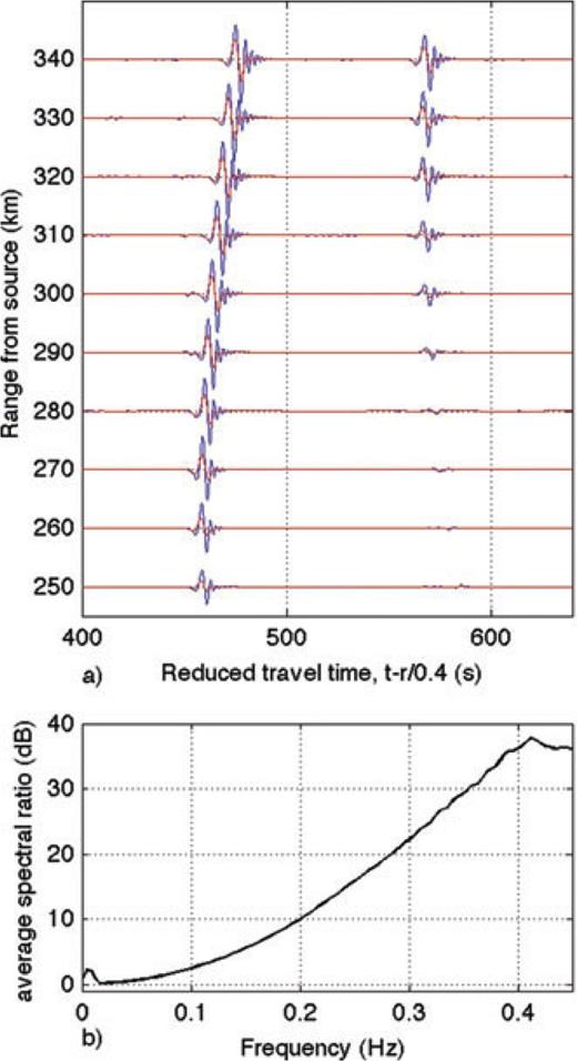
Comparison of thermospheric arrivals. (a) Late arrivals associated with refraction in the thermosphere. The blue lines are the vertical particle motions for the model run with no attenuation, the red lines are the corresponding waveforms for a viscosity coefficient of η= 1.8 × 10⁻⁵ kg m⁻¹ s⁻¹ and bulk viscosity ζ= 0.6 η. (b) Average spectral ratios of non-attenuated versus attenuated waveforms for reduced times 400 s < t_red < 540 s, in dB, at ranges from 250 to 340 km from the source.

Open in new tabDownload slide

A major difference between the observed waveforms and the FDTD waveforms is the absence of tropospherically ducted energy (dWn and uSWn) in the FDTD results (Figs 8 and 9), which show up in the observed waveforms as the first arrivals at all ranges (Fig. 5). Using the ETOPO1 global topography model with a 1.9 km x/y spatial resolution (Amante & Eakins 2009), we recomputed the FDTD waveforms to examine whether the inclusion of topography would explain the observed tropospheric ducting. It did not. We again recomputed the waveforms after altering the model such that the surface was at an elevation of 0 km to examine the effect of a thicker surface duct on the first arrivals. In this case, the synthesized waveforms did indeed result in tropospheric ducting of infrasound energy. We attribute this to the fact that a thicker duct can accommodate lower frequencies than a narrow one; low frequencies are stripped away by a narrow duct (Negraru & Herrin 2009). However, higher frequencies can be trapped within a narrow duct. Thus, this discrepancy between modelled and observed waveforms does not require inaccuracies in the sound and wind speed models, or in the FDTD algorithm. Instead, it may be explained by the fact that we are using a higher frequency band for the observed waveforms for visualization purposes (Fig. 5), and these higher frequencies (relative to the lower frequencies in the FDTD model) can be trapped in the narrow duct near the Earth's surface.

5 Discussion

The large bolide of 2008 that burst above the USArray transportable array, and other dense regional networks in the US Pacific Northwest, provided an opportunity to examine acoustic branches from an impulsive source to several hundred kilometres from the source (Hedlin et al. 2010). In this paper we have taken the next step in this analysis by developing a FDTD code that incorporates winds, attenuation and atmospheric heterogeneity to model propagation from this source and to compare the synthetics with the recorded data.

The first observation from this comparison (observed data in Fig. 5 vs. synthetic data in Fig. 8) is that the first arrivals do not agree very well at ranges beyond about 100 km. Ray theory predicts that these branches result from the ducting of energy in a narrow duct near the surface. However, the entrainment of energy in a narrow duct is frequency dependent, a phenomenon that is not described by ray physics. Acoustic energy with wavelengths greater than the width of the duct is not trapped, while energy at shorter wavelengths (higher frequencies) can be trapped. Thus these differences reflect the fact that the near surface duct is very thin, and that we are comparing high frequency recorded data to lower frequency synthetics. Unfortunately, the high noise levels observed at low frequencies at the USArray stations preclude a direct comparison of observed versus synthetic data at lower frequencies.

However, our primary interest is in comparing thermospherically ducted infrasound energy. As discussed in Hedlin et al. (2010) the two main thermospheric paths from this event are dT, energy down from the bolide and ducted through the thermosphere after a single reflection from the Earth's surface and uT, a simple propagation path up from the source and ducted in the thermosphere. We note that the seismic network recordings from stations at an azimuth of 210° with respect to the north show a thermospheric branch of signals (uT) arriving at about the same time and at the same ranges as predicted by both rays and FDTD computations. This validates the sound and wind velocity models used in this study.

Although the time and range extent of the uT branch agree well, a significant difference between the observed and synthetic waveforms is in the relative frequency content. FDTD computations show that energy refracted in the thermosphere undergoes significant attenuation at frequencies above 0.1 Hz. This is in agreement with our method of integrating predicted infrasound propagation along ray paths (Fig. 7b). However, the data show that there is relatively more high-frequency energy in the thermospheric arrivals than the predictions would suggest. Fig. 5 shows that there is significant energy in the thermospherically refracted infrasound signals in the band from 2 to 8 Hz. Our predictions of attenuation, both from ray paths and from FDTD synthesis, indicate that thermospherically ducted arrivals would have insignificant amplitude at these frequencies. We propose three possible hypotheses:

• 1

  The upper altitude sound speed profiles are incorrect and late arriving energy actually is refracted back to the ground from the lower thermosphere where attenuation is much less severe. This is contradicted by the fact that the observed thermospheric arrivals agree quite well with the predicted arrival times and ranges. The agreement of the timing of the synthetic and recorded branches suggests that sound and wind speed profiles are acceptable, so we discard this hypothesis.

• 2

  Attenuation within the thermosphere is significantly lower than expected, that is, lower than estimates provided by Sutherland & Bass (2004). This implies either that the viscosity coefficient, which has a value on the order of η= 1.8 × 10⁻⁵ kg m⁻¹ s⁻¹ up to elevations of 86 km (Gill 1982), decreases significantly at higher elevations, or that the assumption that the upper atmosphere behaves as a Newtonian fluid is incorrect. This latter assumption was implicit in applying the Navier–Stokes equation (eq. 2) to describe acoustic propagation in a viscous medium. It is possible that infrasound propagation is significantly altered by changes in atmospheric composition with altitude, or that the atmosphere is increasingly ionized at altitudes above about 90 km. In this case, the Sutherland–Bass attenuation model would need improvements to incorporate these effects.

• 3

  Some wavefront steepening occurs as energy propagates to very high altitudes where the ambient pressure is extremely low. At these altitudes the linear assumptions—that the pressure of the sound wave is negligible compared to the ambient pressure and that particle velocities are much lower than the ambient sound speed—may be incorrect. If this is so, non-linear propagation would cause some repopulation of high frequencies. If non-linear effects are indeed significant within the thermosphere the simple linear algorithm used here is insufficient. In this case, a numerical synthesis method incorporating non-linear effects within the upper atmosphere would have to be developed to accurately model infrasound propagation within the atmosphere.

This paper discusses two tools with which to test infrasound propagation physics hypotheses by comparing observations to numerical models. We anticipate that waveform modelling methods of this type may be used to place more accurate limits on wind speeds and acoustic attenuation within the thermosphere and provide tighter constraints on high amplitude sources, both explosions and large volcanic eruptions.

The application of these tools to the study of the Oregon bolide underscores the value of densely sampled infrasound data for atmospheric modelling studies. Although the global infrasound network provides more coverage of the infrasound wavefield than we have ever had before, the network is still very sparse. The infrasound arrays offer precise spot measurements of the true infrasound wavefield, but do not reveal the details of how signals vary with range and azimuth from the source because the average distance between infrasound arrays in the global IMS network is ∼3000 km. With the spatial coverage provided by dense seismic networks, we can map out variations in the infrasound wavefield to test hypotheses governing these arrival patterns with such modelling codes.

6 Conclusions

We have presented the equations relevant to infrasound propagation within a windy medium in which viscosity is the dominant absorption mechanism. The equations do not account for infrasound absorption due to thermal losses or molecular vibration losses, which dominate at lower altitudes but remain negligible at infrasound frequencies. An analytic solution was derived for a wind-less medium with constant density and sound speed, which yields equations for the frequency-dependent phase speeds and attenuation values. These equations are applicable to media with densities and sound speeds that vary at scale lengths much greater than the infrasound wavelength. We assumed that the viscosity coefficient within the thermosphere was approximately equal to its value below 86 km; this estimate results in total attenuation values within the thermosphere that are in close agreement with those derived in Sutherland & Bass (2004) at infrasound frequencies. Under this assumption, we showed that infrasound dispersion is insignificant at altitudes below 120 km at frequencies below 2 Hz, and that attenuation is approximately proportional to the square of the frequency.

We discretized the equations for linear acoustic propagation through an absorptive, heterogeneous, windy atmosphere to develop a FDTD method of synthesizing infrasound waveforms. We describe an FDTD method that is spatially staggered, but centred temporal finite differences are formed over two time steps, as in Ostashev et al. (2005), to retain the accuracy of central differences through a windy atmosphere. Analysis of the numerical accuracy shows that the number of nodes required per wavelength is comparable to the number required for the case where attenuation is not included (e.g. Taflove & Hagness 2000); however, a smaller time step is required to retain accuracy. (Note that we could have used a higher order FDTD approach rather than the first-order staggered grid used. In that case, eqs (15)–(17) would be used as the starting point for further code development.)

Application of the FDTD synthetic modelling to real data shows its utility. We find that standard attenuation models (Sutherland–Bass) predict much greater attenuation within the thermosphere than is observed. We conclude that either the standard attenuation model for the thermospheric is incorrect, or that thermospheric returns are a result of non-linear propagation at very high altitude. In the former case, a better understanding of atmospheric absorption at high altitudes is required; in the latter case, a fully non-linear numerical method is needed to test our hypothesis that higher frequency arrivals from the thermosphere result from non-linear propagation at thermospheric altitudes.

Acknowledgments

The authors are grateful to Douglas Drob of the Naval Research Laboratory for providing the atmospheric specifications used in the propagation modelling, and to David Norris for his careful review. This publication was made possible through support provided by US Army Space and Missile Defense Command. The opinions expressed herein are those of the author(s) and do not necessarily reflect the views of the US Army Space and Missile Defense Command.

References