Very-long-period pulses at Asama volcano, central Japan, inferred from dense seismic observations

Summary

1 Introduction

At volcanoes worldwide, increasing numbers of seismic events consisting of several pulses of 2–100 s in duration are being detected by broad-band seismometers installed near active craters. Such events are often called very-long-period (VLP) pulses and are thought to be generated by volume change and/or mass movement of fluid such as magma, water, or gases. For example, Ohminato (2006) analysed VLP pulses that occurred synchronously with modulations of tremor amplitude at Satsuma-Iwojima volcano, Kyushu, Japan, and proposed a source model in which VLP pulses occur by the sudden vaporization of superheated water. Chouet et al. (2003) proposed a VLP source model in which VLP pulses occur by pressure change caused by the ascent of a gas slug in a volcanic conduit, based on their analysis of VLP pulses that accompanied eruptions at Stromboli volcano, Italy. The latter model was reproduced in a laboratory experiment performed by James et al. (2004) and in a numerical simulation performed by O'Brien & Bean (2008).

VLP pulses are observed at various volcanoes, including high-viscosity dome-growing volcanoes such as Merapi volcano, Indonesia (Hidayat et al. 2000, 2002) and Mount St Helens, USA (Waite et al. 2008); low-viscosity lava-effusing volcanoes such as Kilauea, Hawaii, USA (Ohminato et al. 1998; Almendros et al. 2002); volcanoes with no surface activity, such as Mammoth Mountain, Long Valley, USA (Hill et al. 2002); and volcanoes with explosive activity, such as Popocatepetl volcano, Mexico (Chouet et al. 2005; Arciniega-Ceballos et al. 2008) and Ruapehu volcano, New Zealand (Jolly et al. 2010). Some VLP pulses occur synchronously with surface activity, such as eruptions and gas puffing, whereas others do not, meaning that the mechanisms of VLP pulses might differ among volcanoes. On the other hand, VLP pulses share a number of common features. First, most have rectilinear particle motions directed toward the active crater, suggesting that they consist mainly of P waves and therefore are caused by a pressure source. In addition, most are observed only in the near-field and their source depths are in most cases estimated to be 1 km or shallower. Most of the moment-tensor solutions of VLP pulses obtained to date (e.g. Ohminato et al. 1998; Hidayat et al. 2002; Chouet et al. 2003, 2005; Ohminato 2006; Molina et al. 2008; Waite et al. 2008) are consistent with single or multiple tensile crack source mechanisms, including horizontal sills. Single forces are also often considered (e.g. Jolly et al. 2010). Such similarities among VLP pulses might suggest that VLP pulses at different volcanoes share common source processes.

One problem lying upon analyses of VLP pulses would be the treatment of tilt motions which contaminate horizontal seismograms. As is explained by many literatures (e.g. Rodgers 1968; Aster et al. 2003; Pillet & Virieux 2007), horizontal seismometers are sensitive not only to translational motions but also to tilt motions. This is simply because a tilt motion generates a gravitational force which is equivalent to an inertial force due to a translational acceleration of the ground. Hidayat et al. (2000) demonstrated theoretically that in a near-field observation using broad-band seismometers, a particle motion similar to that of VLP pulses can be obtained from a combination of vertical translational motion and horizontal tilt motion at a node of horizontal translational motion. Aoyama (2008) demonstrated theoretically that the contribution of tilt motion to the horizontal component is as large as 0.6 times that of translational motion in the case of a pulsive source with a duration of 60 s at a depth of 100 m, observed by a CMG40T seismometer at a site located 200 m from the epicentre. Battaglia et al. (2000) and Aoyama & Oshima (2008) are examples of the real tilt signals observed by broad-band seismometers. However, most previous studies of moment-tensor inversions of VLP pulses have been performed based on the assumption that the observed seismograms are wholly translational motions. Although several methods have been proposed to decompose the seismometer record into contributions from translational and tilt motions (e.g. Wielandt & Forbriger 1999; Zahradnik & Plesinger 2005; Graizer 2006), they generally require certain assumptions about the time function or Fourier spectrum of the translational and tilt motions; however, it seems to be difficult to justify such assumptions except for the case in which the ‘correct answer’ is known from other independent observations.

In this study, we developed a new moment-tensor inversion algorithm to deal with tilt signals without decomposing the horizontal seismograms into translational and tilt contributions; instead, we calculate the Green's functions of tilt. The advantage of this approach is that it does not require assumptions regarding ground tilt motion. We applied it to VLP pulses at Asama volcano, central Japan, using broad-band seismograms of up to 14 summit stations.

2 Recent Volcanic Activity and Observations at Asama Volcano

Asama volcano is an andesitic stratovolcano located in central Japan (inset in Fig. 1). It has a summit crater of 450 m in diameter with a summit elevation of 2568 m above sea level; the crater bottom is located at 2312 m above sea level. Two major eruptions have occurred in historical times: the Tenjin eruption in 1108 and the Tenmei eruption in 1783. The volcano was also very active in the 20th century until the early 1960s; after then it became largely quiet, with moderate-sized eruptions in approximately 10- to 20-yr intervals (e.g. Miyazaki 2003).

Figure 1

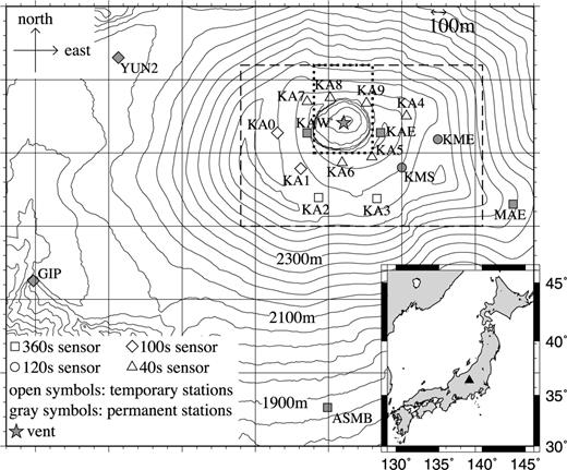
Station layout at the summit area of Asama volcano. Squares, circles, diamonds, and triangles indicate Guralp CMG-3T 360 s sensors, Nanometrics Trillium 120 s sensors, Guralp CMG-3T 100 s sensors, and Nanometrics Trillium 40 s sensors, respectively. Open and grey symbols indicate temporary and permanent stations, respectively. The star indicates a vent at the crater bottom, as determined from orientation measurements from station KAW and from three additional sites on the crater rim. The dashed rectangle indicates the area within which stations were used in the present waveform analysis. The dotted rectangle indicates the area shown in the map in Fig. 8. The triangle in the inset indicates the location of Asama volcano.

Open in new tabDownload slide

After a 21-year-long quiescence, Asama volcano experienced moderate-sized vulcanian eruptions in 2004 (e.g. Yoshimoto et al. 2005). The first eruption, on September 1, was preceded by the intrusion of a dyke several kilometres west from the summit in the late 2004 July (Aoki et al. 2005), and by an earthquake swarm 1 d before the eruption (Yamamoto et al. 2005). Takeo et al. (2006) relocated earthquakes and indicated the magma supply path beneath the volcano, connecting the dyke detected by Aoki et al. (2005) and the current summit crater. The dyke and the magma supply path was consistently supported by recent seismic (Aoki et al. 2009) and magnetotelluric (Aizawa et al. 2008) surveys of the subsurface structures. Asama volcano also erupted in 2008 August and after 2009 February. The 2009 activity created a vent near the crater centre (star in Fig. 1), with several tens of metres in diameter, from which distinct slow gas emission events are frequently observed.

At the summit area of this volcano, VLP pulses (Fig. 2) are observed. In this and later figures, and in all the analyses, the seismometer's responses were corrected into Nanometrics Trillium 120 sensor's response unless being stated otherwise. The occurrence rate of the VLP pulses have been quite stable, with approximately 10 events per day in average (Fig. 3). However, it gradually decreased and finally disappeared before the 2004 September 1, eruption, regardless of the trend in the occurrence of ordinary volcanic earthquakes (Yamamoto et al. 2005). This change in seismic activity coincided with the timing of dyke intrusion (Aoki et al. 2005) in late 2004 July, suggesting that a certain change in, for example, stress field or thermodynamic condition at shallow levels beneath the crater, caused by intrusion of the dyke, might have influenced the occurrence of VLP events. During the eruptive activity in 2008, the daily frequency of VLP pulses increased before the eruptions (Fig. 3). In addition, VLP pulses with long (∼50 s) durations took place about 3 min before all the three small eruptions in 2008. VLP pulses recorded after 2009 May preceded distinct slow gas emission events by approximately 30–60 s (Fig. 2c). These observations suggest that the source process of VLPs is related to gas movement at shallow levels within Asama volcano.

Figure 2

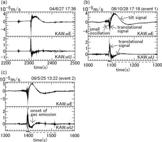
(a) Event that occurred at 17:38 on 2004 June 27. Origin of time (t= 0) is 17:00 on the event day. (b) Event that occurred at 17:18 on 2008 October 28, hereafter referred to as ‘event 1’. Origin of time (t= 0) is 17:00 on the event day. (c) Event that occurred at 13:22 on 2009 May 25, hereafter referred to as ‘event 2’. Origin of time (t= 0) is 13:00 on the event day. The upper and lower sub-panels in each panels are east–west (near inward radial) and up–down components at station KAW, respectively. Black solid lines and grey dashed lines at the bottom of panels (b) and (c) denote time windows plotted by orange and blue lines in Fig. 7, respectively.

Open in new tabDownload slide

Figure 3

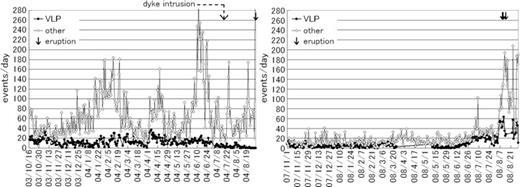
Daily frequency of VLP pulses at Asama volcano (closed circles) during the period before the first of the 2004 eruptions (left-hand panel) and after re-installation of the summit stations in 2007 (right-hand panel), together with that of non-VLP volcanic earthquakes (open diamonds). Eruption timings are indicated by arrows. Timing of dyke intrusion shown in the left-hand panel was determined by Aoki et al. (2005).

Open in new tabDownload slide

We have no VLP data between 2004 September and 2007 October because the summit station was broken by the eruption. Although there had been no broad-band summit record before 2003 October, Yamamoto et al. (2005) found that similar impulsive events had occurred previously, at least since 2002 September 5, by removing the short-period seismometer's response at KAW; prior to this period, the data quality was too low to carry out similar analyses.

In order to study the source mechanism of these events, we made a dense temporary seismic observation, which is explained in the next section. Then, several characteristics of the VLP pulses are described in Section 4. Next an explanation of the inversion procedure is given in Section 5. This is the new inversion algorithm to include tilt signals which contaminate the horizontal seismometers. In Section 6, the inversion result of a representative VLP event that occurred at 17:18 on 2008 October 28 (Fig. 2b), is described. Throughout this paper, this event is referred to as ‘event 1’. In addition to the analysis of event 1, inversion analyses were conducted for additional 22 events (Fig. 4), and comparison of the results is given in Section 7. This approach may be a bit different from several previous studies. In several previous studies (e.g. Ohminato 2006) a waveform similarity among events was first checked, then a stacked waveform was prepared to improve signal-to-noise ratio, and then an inversion was performed for the stacked waveform. In this study, signal-to-noise ratios of many of the events are sufficiently high, and thus stacking is not necessary. A merit of the event-by-event analyses approach, which was adopted in this study, is to avoid making an assumption that the events occurred by a common source mechanism at a common source location. Even if the waveforms among events are similar to each other, the source mechanisms and locations among them can be different to each other because, in near-field observation, the mechanisms and locations are mainly reflected to the radiation pattern; not to waveform. Now that we have an efficient frequency-domain inversion algorithm, together with more and more high-spec computers, time required to analyse many events would not be a serious problem. We therefore first analysed many events and after then compared the results among them. Correlation analysis is given in Appendix B. Another named event, ‘event 2’, appears in this paper, to indicate an event that occurred at 13:22 on 2009 May 25 (Fig. 2c). Inversion analysis for this event was not conducted because it occurred out of the temporary observational span. However, it is followed by a distinct slow gas emission event, thus comparison of waveforms and particle motions between this event and analysed events plays an important role in interpretation.

Figure 4

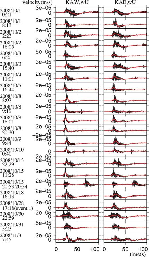
Vertical seismograms of analysed events at stations KAW (left-hand panels) and KAE (right-hand panels). Black lines are raw seismograms; red lines are low-pass-filtered seismograms with a corner frequency of 0.1 Hz.

Open in new tabDownload slide

3 Observation

Fig. 1 and Table 1 shows the seismic network used in this study. We used four permanent stations (KAE, KAW, KME and KMS) and 10 temporary stations (KA0–KA9). All 14 stations are three-component broad-band sensors located within 1 km of the crater; composed of two Guralp CMG-3T 360 s sensors, two Nanometrics Trillium 120 s sensors, two Guralp CMG-3T 100 s sensors and six Nanometrics Trillium 40 s sensors. Data recorded at stations located farther from the crater, including MAE, YUN2, GIP and ASMB in Fig. 1, were not used because VLP signals at these stations were too weak to be used for analyses (Fig. 5). The station layout was determined by synthetic estimates of resolutions of the moment-tensor solutions. For more detail, see Appendix A.

Table 1

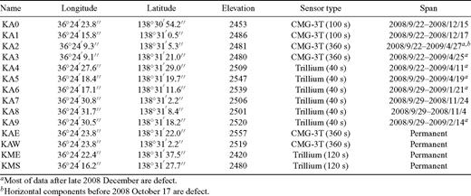
Information of stations used in this study. Coordinates are represented by WGS datum and elevations are represented by metres above sea level.

Open in new tabDownload slide

Figure 5

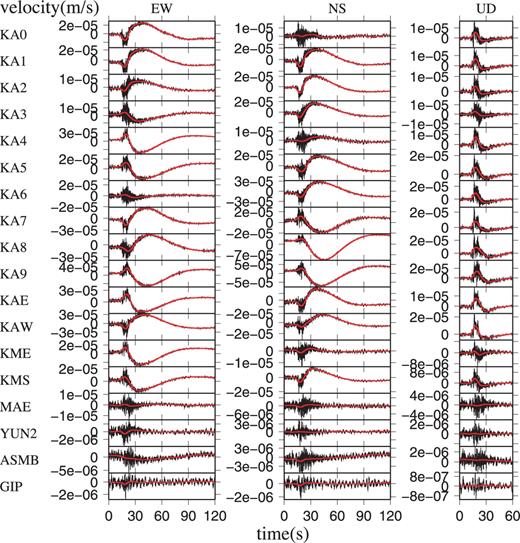
Seismograms of the ‘event 1’ VLP in Fig. 2(b), as observed at various stations. Black lines represent the raw seismograms and red lines represent the low-pass-filtered seismograms with a corner frequency of 0.1 Hz.

Open in new tabDownload slide

The permanent stations are fed by an AC electric power supply and data are transported to the observatory using a Local Area Network over an optical fibre cable network in real time. The temporary stations were powered by solar panels connected to chargeable car batteries. Data were stored on flash memory mounted on a Datamark LS-7000XT data logger (Hakusan Co., Japan). The temporary observation was carried out between 2008 September and 2009 April, and sufficient data are only available for 2008 (Table 1). The sampling rate and dynamic range of discretization were set to 100 Hz and 24 bit, respectively, except for a period of 200 Hz sampling by temporary stations between 2008 October 17 and November 4, with the aim of determining the source locations of high-frequency earthquakes.

4 Seismograms, Spectra, and Particle Motions

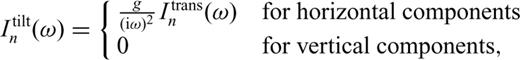
Fig. 5 shows a VLP event (event 1) observed at broad-band stations within 2 km of the crater. The seismograms recorded at stations within 1 km of the crater (upper 14 panels in Fig. 5) show similar characteristics to each other. Also, seismograms among the VLP events are quite similar to each other, as is indicated by high values of cross correlations among them (Appendix B). The VLP events start with an upward and outward velocity motion with amplitudes of less than the order of 10⁻⁴ m s⁻¹ and with typical durations of 10–20 s, followed by smaller and slightly longer translational signals with an opposite sign (lower subpanels of Fig. 2). Horizontal seismograms are contaminated by much longer transient signals (upper subpanels of Fig. 2). Theoretically, tilt motion contaminates horizontal seismograms as a first order term while it affects vertical seismograms as a second order term; thus contamination from tilt motions on vertical seismograms can be neglected for ordinary microradian-order tilts (e.g. Pillet & Virieux 2007; Aoyama 2008). Since the transient signals after the VLP pulses appear exclusively in horizontal seismograms at all the 14 stations (Fig. 1), having various incidence and azimuthal angles, they seem to be generated by tilt motions. Some VLP pulses are up to 30–50 s in duration, being composed of multiple subpulses.

The right-hand panels in Fig. 6 show examples of Fourier amplitude spectra for a VLP pulse (black lines) and noise (grey lines). Signal and noise spectra were calculated using 1000-s-long windows encompassing the VLP pulse and the preceding background noise, respectively. The upper half of Fig. 6 shows radial and vertical Fourier spectra recorded at a CMG-3T 360 s station (KAE), as the broadest end-member of the sensors used in this study. The lower half of Fig. 6 shows radial and vertical Fourier spectra recorded at a Trillium 40 s station (KA4), as the narrowest end-member of the sensors used in this study. In this figure, the seismometer's responses were not corrected. This figure shows that the available frequency range of the VLP analysis is 0.005–0.1 Hz. The frequency range lower than 0.005 Hz is dominated by noise, especially for vertical components, due to the observational limitations of the seismometer. Even for the vertical component of Trillium 40 s sensors, frequencies above 0.005 Hz (200 s) are dominated by signal rather than noise. This is the reason why we decided to correct the seismometer's responses to the Trillium 120 s sensor's response in order to make use of frequencies below 0.025 Hz (40 s) and to cut out the frequencies below 0.005 Hz (200 s). Contamination from noise in the frequency range above 0.1 Hz, which probably represents microseismic noise, is avoided by low-pass filtering with a corner frequency of 0.1 Hz.

Figure 6

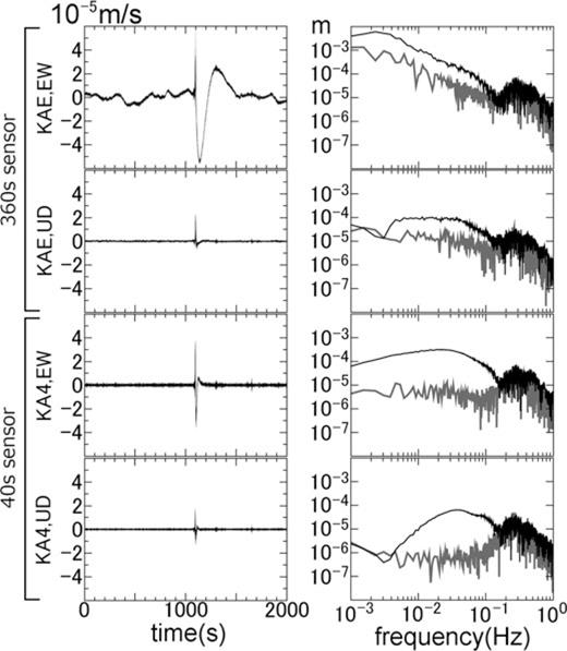
Fourier amplitude spectra for event 1 in Fig. 2(b). The grey lines in the right-hand panels show the Fourier amplitude spectra for a time window of 0–1000 s (the first half of the left-hand panels), which represent noise spectra immediately before the VLP pulse. The black lines in the right-hand panels show the Fourier amplitude spectra for a time window of 1000–2000 s (the latter half of the left-hand panels), which include the VLP pulse. The seismometer's responses were not corrected.

Open in new tabDownload slide

Fig. 7 shows particle motions for events 1 and 2. The orange lines show particle motions in a time window in which the vertical components of the seismometers recorded a clear VLP signal and in which the horizontal seismograms resembled vertical ones, suggesting that the seismograms in this time window are dominated by translational signals. The blue lines show particle motion in a time window after the clear vertical signals had disappeared and in which the horizontal longer-duration signals persisted, suggesting that the seismograms in this time window are dominated by the horizontal seismometer's response to tilt motions; recall that tilt signals appear exclusively in the horizontal components. Of course, both signals may co-exist in both time windows; this division of time windows is simply a matter of convenience. Despite that particle motions for all the stations used in analysis are rectilinear and point in the direction of the crater, they do not point to a single location in the crater, especially in the case of the tilt signals indicated by blue lines. For example, the particle motion at KA0 points eastward, whereas the particle motion at KAW points northeastward. A similar discrepancy is seen between KME and KAE, and the particle motions at KME and KA4 do not appear to intersect with each other within the crater. Tilt directions are radial directions in the case of an isotropic and sufficiently small source located in a homogeneous medium under a flat free surface (Mogi 1958). Therefore, the discrepancies in the directions of tilt signals among the stations must reflect either a non-isotropic source, a finite source size, non-flat topography, an inhomogeneous medium, or some combination of these factors.

Figure 7

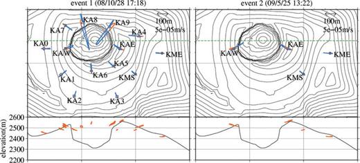
Particle motions for events 1 and 2 in Fig. 2. For event 1 (left-hand panel), orange and blue lines correspond to time windows of 1085–1100 s and 1100–1295 s in Fig. 2(b), respectively. For event 2 (right-hand panel), orange and blue lines correspond to time windows of 1390–1405 s and 1405–1520 s in Fig. 2(c), respectively. Projections of particle motions to the horizontal plane are indicated in the upper panels; projections to an east–west cross-section are shown in the lower panels. For east–west cross sections, only the orange lines are plotted, as particle motion in time window of the blue line in vertical plane appear to be strongly biased by tilt signals exclusively appear in horizontal seismograms. The green dashed lines in the upper panels indicate the section line along which topography is plotted in the lower panels. A 0.1 Hz low-pass filter was applied before plotting this figure.

Open in new tabDownload slide

5 Moment-Tensor Inversion Including Tilt: Method and Conditions

Fourier spectrum of observed seismogram generated by a point source moment-tensor can be represented as

1

where ω is the angular frequency; p is a direction of force; q is the direction of the arm of the moment-tensor; n is a consecutive number which uniquely indicates a combination of station and component; ‘_q’ is the partial derivative with regard to the coordinate x_q; U^obs_n(ω) is the Fourier spectrum of the nth seismogram; I^trans_n(ω) and I^tilt_n(ω) are the nth seismometer's responses to translational and tilt motions, respectively; G^trans_np(ω) and G^tilt_np(ω) are the Fourier spectra of nth component of Green's functions for translational and tilt motions, respectively, excited by a unit impulse oriented in pth direction; and M_pq(ω) is the Fourier spectrum of the moment-tensor solution, which we aim to derive by the inversion. Here, the summation convention for repeated subscripts is applied. For derivation of eq. (1), see Maeda et al. (2011). A key improvement of this study is to consider the second term in the braces of the right-hand side of eq. (1) while this term has been ignored in previous studies. By this method, decomposition of the observed seismogram U^obs_n(ω) into translational and tilt contributions is not required, and instead the tilt effect is considered by including it to the braces of the right-hand side of eq. (1).

In practice, it is more convenient to use

2

where S₀(ω) is the Fourier transformation of a known arbitrary source time function used to calculate a synthetic displacement S₀(ω)G^trans_np,q(ω) and a synthetic tilt S₀(ω)G^tilt_np,q(ω). Calculation of the Green's functions G^trans_np,q(ω) and G^tilt_np,q(ω) themselves is impossible; they are purely the theoretical functions which can not be numerically obtained for arbitrary 3-D topography and structure. Instead we can numerically calculate S₀(ω)G^trans_np,q(ω) and S₀(ω)G^tilt_np,q(ω), which will be referred to as ‘practical Green’s functions', in order to avoid confusion between those convolved with and without S₀(ω). Eq. (2) can be written in the ordinary linear inversion form

3

where d(ω) is the data vector and m(ω) is the model vector, respectively, defined as

4

and

5

where N is the number of observed seismograms, and the superscript T denotes transpose of matrix. The data-kernel matrix G(ω) is composed of the braces of the right-hand side of eq. (2); explicit form of this matrix can be easily derived by equations given above.

We can obtain I^trans_n(ω) from information on poles and zeroes of the seismometers, and I^tilt_n(ω) can be calculated as

6

where g is the gravitational acceleration and i is the imaginary unit. For derivation of eq. (6), see Aoyama (2008) or Maeda et al. (2011), for example. We previously developed a finite-difference method (FDM) code to calculate the practical Green's functions of both translational and tilt motions in Maeda et al. (2011). This FDM code is essentially based on that proposed by Ohminato & Chouet (1997), in which arbitrary 3-D topography and structure can be included with a usage of staggered-grid scheme. The grid cells belong either to solid or vacuum domains, and grid interfaces shared by the both type of grid cells are regarded to be the approximated free surface, on which zero-traction free surface condition is satisfied by putting the Lame's coefficients in the vacuum cells to zero. In order to calculate long-duration synthetic seismograms, we combined the FDM code with Perfect Matched Layer (PML) absorbing boundaries proposed by Festa & Nielsen (2003). From the numerical tests performed in Maeda et al. (2011), numerical error of up to 10 per cent occurs mainly by usage of a finite grid size, while reflected waves from numerical boundaries are far smaller than this error, for conditions quite similar to this study.

Many of the previous moment-tensor inversion studies at volcanoes (e.g. Ohminato et al. 1998, 2006; Chouet et al. 2003) have considered single-force source mechanisms in addition to the moment-tensors. However, consideration of the single-forces results in an increase of the degree of freedom, by which a problem regarding resolution or uniqueness of the solution would arise. Since the waveforms of the VLP pulses at Asama volcano were well reconstructed without considering the single forces, as is indicated in the later section, we do not consider the single force. While the single-force source mechanisms were often interpreted as a reaction force to explosion (e.g. Kanamori et al. 1984) or drag force caused by movement of viscous magma (e.g. Ukawa & Ohtake 1987), the VLP pulses at Asama volcano can be interpreted without considering such processes; the only movement required to explain the source process is a gentle movement of non-viscous gas, as is described later.

Table 2 summarizes the parameters and conditions used in calculating the practical Green's functions. Referring to Aoki et al. (2009), a linearly increasing P-wave velocity structure with regard to depth was used for calculation of the practical Green's functions, from Vp= 2.0 km s⁻¹ at 2500 m above sea level to Vp= 4.0 km s⁻¹ at sea level. Because we had no information on S-wave velocity, we assumed V_s = V_p/√3. A uniform density of ρ= 2500 kg m⁻³ was assumed. A 10-m-mesh digital elevation model (DEM) was included and a 0.001 s time interval was adopted to stabilize the calculation. Conditions for PML were chosen based on the results of numerical tests performed by Maeda et al. (2011). A source time function of the form

7

with τ_p= 5 s was input, which is the unique polynomial of minimum possible degree that satisfies the following conditions: (1) zero before t= 0, (2) unity after t=τ_p, (3) monotone, and (4) second-order derivatives are continuous. Conditions (1) and (2) are the requirements to represent a source process that have a residual moment-tensor, which seems to be appropriate for cases where volumetric expansion of gas is assumed. Condition (3) is only for simplicity. Condition (4) is required so that far-field-term velocities are continuous with regard to time; this continuity is required because we use velocity expression in the FDM code. Anyway, choice of the source time function S₀(t) to calculate the practical Green's functions is not important, as long as it does not to result in the low accuracy in the FDM calculation; recall that S₀(t) is eliminated in the inversion process, as is indicated by eq. (2).

Table 2

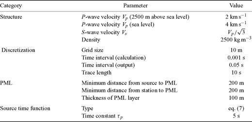
Parameters and conditions employed in calculation of the practical Green's functions.

Open in new tabDownload slide

In order to save calculation cost, the reciprocity theory was applied, like many of the previous inversion studies (e.g. Chouet et al. 2003); sources are input at the station locations and wavefield are calculated at candidate source locations. This approach reduces the number of calculations, in cases where a grid-search for numerous candidates of the source locations is planned. In our case, every x-, y- and z-components of translational Green's functions, and x- and y-components of tilt Green's functions, at every 14 stations, were individually calculated. In calculating the tilt Green's functions, a smoothing by averaging them at five adjacent grid cells in station side was applied, based on our numerical tests reported in Maeda et al. (2011). This does not result in an increase of number of calculations required; instead of calculating the tilt Green's functions for each adjacent grid cells separately, a reciprocity source for the averaged tilt was input instead. In some stations, tilt could not be defined at some of the adjacent grid cells [see appendix of Maeda et al. (2011)]; in such cases, such grid cells were not used for average.

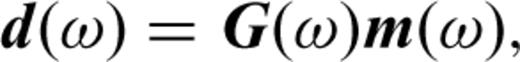
Eq. (3) was inverted using a singular-value decomposition method (e.g. Menke 1989). A criterion was adopted that singular-values smaller than 0.01 times the maximum singular-value were regarded to be effectively zero. However, in applying this criterion, all the singular-values in the inversions were non-zero, meaning that the inversion solutions were the same as the least-squares solutions. The inversions involved no weight matrix, damping factor, nor other a priori constraints, and numerical stability was ensured by application of the singular-value decomposition method.

Before carrying out the inversions, the data were converted to the response of the Nanometrics Trillium 120 s seismometer, resampled at 2 Hz, subtracted by the initial value of the time window, subjected to cosine tapering for the last 300 s of the 660-s-long time window, padded by zeroes into a 2048-s-long trace, and finally subjected to a Fourier transformation. We then performed the inversions for each discretized frequency from 0 to 1 Hz with a frequency interval of 1/2048 Hz. We carried out inversions for each of the candidate source locations indicated by symbols in Fig. 8, and searched for the best source location which returned the minimum square error between the observed and synthetic seismograms low-pass filtered with a corner frequency of 0.1 Hz, four poles, and zero phase shift. Since this grid interval (50 m) resulted in sufficiently small differences in residuals between adjacent candidate source locations, we concluded that a smaller spatial grid-search interval was not required.

Figure 8

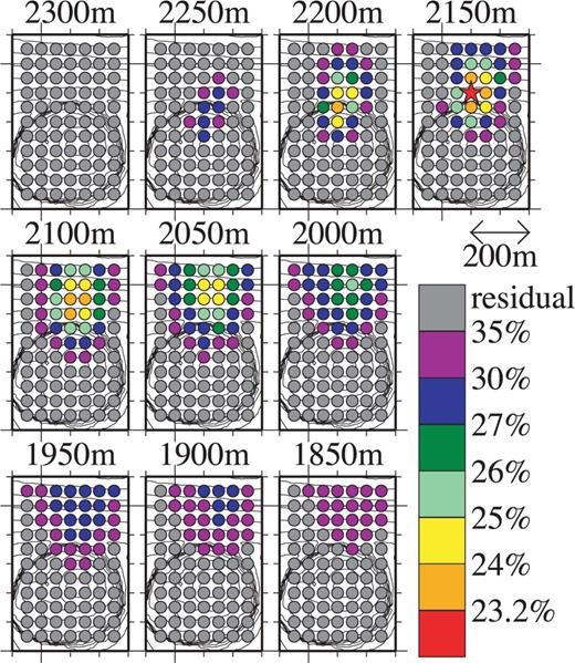
Horizontal cross-sections of the spatial distribution of the residuals of event 1, as defined by eq. (8). The horizontal range of the map is indicated by the dotted rectangle in Fig. 1. The elevation of each cross-section is indicated at the top of the panel, in metres above sea level. The best-fitting source location is indicated by the red star. The colour scale employed to indicate the range of residuals is common for both the circles and the star.

Open in new tabDownload slide

6 Analysis of a VLP Pulse that Occurred at 17:18 on October 28, 2008 (Event 1)

While residuals d(ω) −G(ω)m(ω) can easily be obtained by the inversion process, they depend on frequency; thus single ‘best-fitting’ source location is not determined by comparing these frequency-dependent residuals. Instead, we compared the following residual

8

for each candidate source locations, which is not a function of frequency. Here, Δt is the sampling interval of data used in the inversion (0.5 s in this case), and v^obs_n(t) and v^syn_n(t) are the observed and synthetic velocity seismograms, respectively, low-pass filtered with a corner frequency of 0.1 Hz. Of course the tilt effect was included in the synthetic velocity seismograms. Fig. 8 shows the residuals for event 1, calculated by eq. (8), indicating that the best-fitting source location (the red star) lies outside of the crater. However, since differences in residuals among neighbouring locations are small, the source location would have an uncertainty of 50–100 m in each direction. Even after taking this uncertainty into account, the source location is clearly located north of the crater centre and its depth is 100–300 m (elevation is 2200–2000 m).

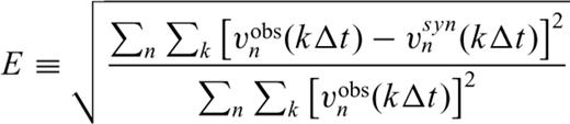
Fig. 9 compares the observed (red lines) and synthetic (blue lines) filtered waveforms, and Fig. 10 shows their particle motions. The east–west component at KA6 and the north–south components at KA0, KA4 and KME are nearly transverse components and their amplitudes are small. In addition, the up–down components are small at KME and KMS. Other than these small traces, we see some non-systematic slight discrepancies, mainly in the horizontal components, but overall the vertical and horizontal seismograms are well reconstructed. The discrepancies might arise from the point source approximation. However, we opted not to consider an extended source model; instead, we sought to interpret the best-fitting point source model as a first approximation.

Figure 9

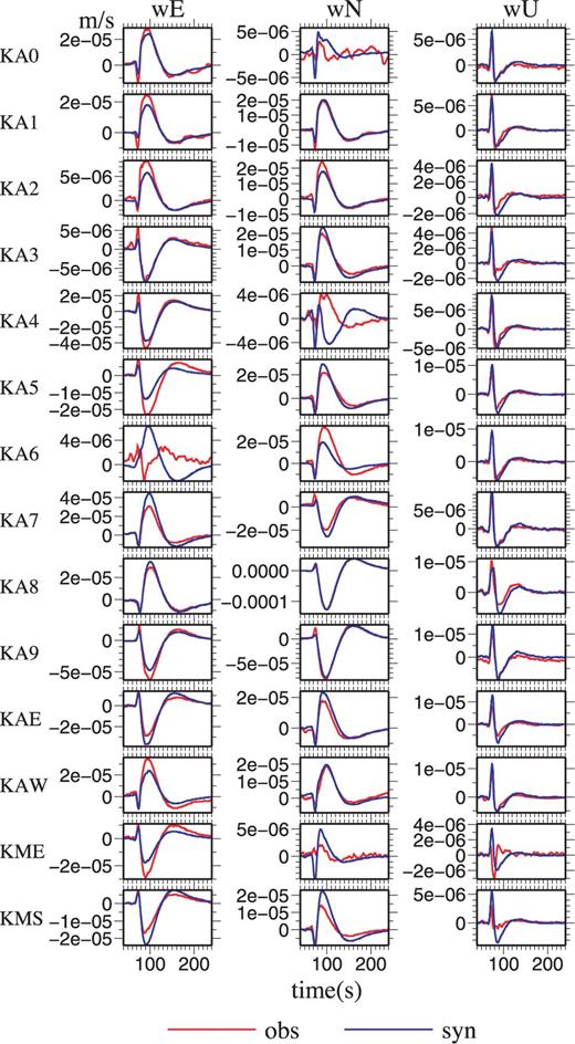
Comparison of observed seismograms (red lines) and synthetic seismograms (blue lines) for event 1 with a four-pole zero-phase Butterworth low-pass filter at 0.1 Hz.

Open in new tabDownload slide

Figure 10

The same data as Fig. 9, projected to the horizontal plane (the upper panel) and to an east–west cross-section (the lower panel). Dashed line in the upper panel indicates a section line along which topography is plotted in the lower panel.

Open in new tabDownload slide

Fig. 11(a) shows the moment-tensor solution for event 1. Here, the x-, y- and z-axes correspond to directions to the east, north, and upward, respectively. The moment-tensor time histories are similar among the components, consisting of an initial rapid inflation phase and a subsequent gradual deflation phase. This similarity enables us to define a focal mechanism not as a function of time but as a unique mechanism for the event. The amplitude of each of the six moment-tensor components of this event was determined as the difference between the peak value near t= 80 s and the value at t=−50 s (time before the event), yielding

9

Here, the M_zx component was set to zero because this component had a negligible amplitude and a markedly different time function from that of the other components. This moment-tensor had eigenvalues (principal values) of (5.598, 3.387, 2.260) × 10¹² N m, whose eigenvectors (principal axis) are indicated in Fig. 11(b). The length of the principal axes were chosen to be proportional to the corresponding principal values, and were projected onto a horizontal cross-section, an east–west cross-section, and a north–south cross-section.

Figure 11

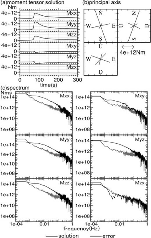
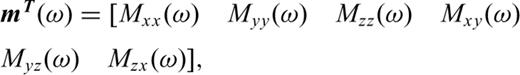
(a) Moment-tensor solutions for event 1. The x-, y- and z-axes represent directions to the east, north, and upward, respectively. (b) Projection of the principal axes of moment-tensor amplitudes of event 1 into a horizontal plane (upper left-hand panel), an east–west cross-section (lower panel) and a north–south cross-section (right-hand panel). All the principal values are positive and line lengths are proportional to the principal values. (c) Fourier amplitude spectra of the moment-tensor solutions for event 1 (black lines) along with their errors (grey lines).

Open in new tabDownload slide

Fig. 11(c) shows the Fourier amplitude spectra of the moment-tensor components of event 1 (black lines), together with their error estimates (grey lines). Here, the errors were defined as square roots of the diagonal components of the model covariance matrices, as follows:

10

where [covd] is the data covariance matrix, G^−g is the generalized inverse of the data-kernel matrix, and the superscript T is the transpose of the matrix (e.g. Menke 1989). Here, the generalized inverse is defined as a matrix which satisfies the following:

11

where d and m^est are the data vector and estimated model vector, respectively. The generalized inverse was calculated as

12

where p denotes number of non-zero singular-values; Λ_p is a p-times-p diagonal matrix composed of non-zero singular-values; U_p and V_p are matrices composed of p singular-vectors in data-space and model-space, respectively, corresponding to each non-zero singular-values; and the superscript T denotes transpose of matrix (Menke 1989). Regarding [covd(ω)], we assumed that the off-diagonal components are zero and used squares of the Fourier spectra for the noise part (0–1000 s) in Fig. 6 as their diagonal components. Indeed, since the data vector used in the present inversion is convolved with the source time function, we multiplied the spectrum of the source time function by the original noise spectra and used their squares as the variance of the data. From Fig. 11(c), we can confirm that the moment-tensor solution is well reconstructed in the frequency range of 0.002–0.1 Hz (500–10 s). Considering that up to 6 sensors among 14 were the 40 s sensors, we can recognize that frequency of as low as 500 s was reconstructed owing to the usage of the tilt signals. For the M_zx component, almost all the frequencies are close to the noise level, meaning that M_zx is less than or equal to the noise level.

7 Comparison of Results Among Events

To obtain a statistical perspective of the source mechanisms of the VLP pulses at Asama volcano, we performed moment-tensor inversions for 23 events (Fig. 4) that occurred between 2008 September 29 and November 4. In selecting these 23 events, we aimed to include a varieties of events, including short- and long-duration events, and one- and multi-pulse events. Some of the analysed events (8:07, 9:19 and 20:30 on October 8, and 0:40 on October 10) had inconsistent time histories among the moment-tensor components, indicating time-variant source mechanisms. However, for remaining 19 analysed events, the moment-tensor time histories among components were consistent with each other, enabling determination of the time-invariant source mechanisms. Representative parameters, showing the results of analyses of these 19 events, are compiled in Fig. 12. Source locations for all the analysed events are near the northern crater rim, with elevations between 2100 and 2200 m above sea level (Figs 12a–c). The parameters M₁, M₂ and M₃ in Fig. 12 indicate the largest, intermediate, and smallest principal values, respectively. The ratios M₂/M₁ (Fig. 12d) and M₃/M₁ (Fig. 12e) yield values near 0.55 and 0.4, respectively. In previous studies of VLP pulses at other volcanoes (e.g. Chouet et al. 2003; Ohminato 2006), similar mechanisms have been approximated as 2: 1: 1, and interpreted as a tensile crack with λ= 2μ. In our case, however, second and third principal values are obviously different to each other, based on inversions of up to 23 events with sufficient resolutions (Figs 12d and e). Some minor correction from simple tensile crack source mechanism may be more appropriate. If λ=μ is assumed, and the M₂/M₁ value is approximated to 0.6, then the principal value ratio M₁: M₂: M₃ is 5: 3: 2, which can be interpreted as the synchronized volumetric change of a tensile crack and a cylinder with symmetry axes oriented orthogonal to each other, namely, 5: 3: 2 = 3: 1: 1 (tensile crack) +2: 2: 1 (cylinder). Also, 2× (3: 1: 1 (tensile crack)) +2:2:1 (cylinder) =8: 4: 3 = 1: 0.5: 0.375 is near to Figs 12(d) and (e). Therefore, although possible interpretation is not unique, a synchronized volumetric change of a tensile crack and a cylinder may be one possible interpretation of the result.

Figure 12

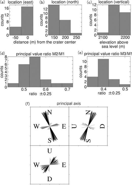
Histograms (a–e) and principal axes (f) showing the inversion results of all the analysed events. M1, M2 and M3 in panels (d) and (e) are the largest, intermediate, and smallest principal values, respectively. In panel (f), lengths of the lines are normalized by the rms lengths for each events. Black, dark grey and light grey lines indicate the largest, intermediate and smallest principal axes, respectively. Only the 19 events with consistent moment-tensor time histories are shown for panels (d)–(f).

Open in new tabDownload slide

Fig. 12(f) summarizes principal axes for all these 19 events. In the ‘tensile crack plus cylinder’ model, the largest principal axes (black lines) represent orientations normal to the tensile cracks, and the smallest principal axes (light grey lines) represent the directions of the symmetry axes of the cylinders. They have small variations; strikes and dips of the cracks are both concentrated on near 70°, while cylinder axes are typically inclined by 30° from vertical and horizontally rotated by 60° from x-axis in counter-clockwise. Typical source locations and orientations of crack and cylinder are schematically shown in Fig. 13, although sizes of the crack and the cylinder are unknown.

Figure 13

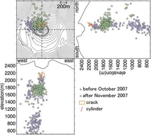
Relationship among the inversion results, surface topography and hypocentres of non-VLP volcanic earthquakes. The upper left-hand panel, lower panel and right-hand panel show projections into the horizontal cross-section, an east–west cross-section, and a north–south cross-section, respectively. Topographies plotted in the vertical sections are those along the black dashed lines in the map view. Orange solid quadrangle indicates a representative tensile crack of the VLP source, while red dotted line indicate a representative symmetry axis of cylinder of the VLP source. Sizes of crack and cylinder are unknown; a crack of 150 m long and 100 m wide and a cylinder of 200 m long are assumed. Hypocentres are shown for ordinary earthquakes with latitudes (lower panel) and longitudes (right-hand panel) within 300 m of the black dashed lines and with altitudes (upper left-hand panel) higher than 500 m above sea level. These hypocentres were determined using the double-difference method proposed by Waldhauser & Ellsworth (2000). Because the installation of summit stations in early 2007 November may have affected the hypocentre distributions, different symbols are used for data collected before and after installation of the stations.

Open in new tabDownload slide

8 Discussion

8.1 Stability of the solution

Although the resolution of the moment-tensor solutions were good, as is inferred from the fact that all the singular-values were non-zero, this can be said only when the source location is fixed. Indeed, there is a trade-off between the source location and the moment-tensor solution. For example, the source mechanism of event 1 for a location 50 m east from the best-fitting location is different from the best-fitting model indicated in Figs 11(a) and (b), in that the sign of M_xy is opposite and correspondingly the largest principal axis is oriented in northeast–southwest direction. Since the difference in residual between these two locations are small (Fig. 8), it is not clear which solution is really better. In order to obtain a perspective view of the trade-off, we compared moment-tensor solutions of all the analysed events, for some of the alternative source locations: for event 1, solutions at all the candidate source locations within 100 m in each directions from the best-fitting location were checked; and for remaining 18 events which have consistent moment-tensor time histories among components, solutions between at the best-fitting locations and at 50 m eastern locations were compared. The comparison clearly showed that the moment-tensor solutions at the north of the crater centre (and at western locations) generally had negative M_xy, indicating northwest–southeast oriented largest principal values. On the other hand, the solutions at locations 50 m east (and of course near the northern rim) of the crater centre generally had positive M_xy, indicating northeast-southwest oriented largest principal values. Principal value ratios at both the locations were similar to each other. Probably, the results were strongly affected by KA8 and KA9, where amplitudes were relatively large. Indeed, orientations of the largest principal axis, at locations just north of the crater centre and 50 m east, were near to particle motion directions at KA8 and KA9, respectively. In addition, fittings of horizontal components of KA8 were better for the former locations, while those of KA9 were better for latter locations. Probably, the real source had a finite size, and stations (especially KA8 and KA9) were too near to the source for point source approximation.

Another problem may be the effect of velocity structure used in this study. Bean et al. (2008) and O'Brien et al. (2010) indicated that an incorrect shallow velocity structure may read into a wrong moment-tensor inversion result, for a case of LP (∼1 Hz) event observed by a seismic network of a few kilometer order. In order to estimate the effect of velocity structure for a case of the VLP pulses at Asama volcano, having a duration of ∼10 s and a seismic network of a few hundred metres order, a numerical test was conducted. A known moment-tensor source, indicated by the green solid lines of Fig. 14(a), was input at the best-fitting location of event 1, and synthetic seismograms at all the 14 stations were generated, using the same FDM code as that used to produce the practical Green's functions. At this stage, three velocity structure models were used (Table 3); Structure 1 was a model having velocities by 25 per cent faster than the structure assumed in the inversion; Structure 2 was a model having velocities by 25 per cent slower than the structure assumed in the inversion; and Structure 3 was a model having similar velocity values at summit area, but different from the model assumed in inversion in that the Structure 3 velocity model is uniform, that is, velocity does not increase with depth. In generating these synthetic seismograms, 3-D topography was included and both translational and tilt motions were considered. Then, the same inversion analyses as Section 5 were conducted for these synthetic waveforms, with a use of the velocity structure indicated in Table 2. The resultant moment-tensors were expected to be different from the input source, because of the difference between the velocity structure used in generating the synthetic seismograms and that used in calculating the practical Green's functions. The best-fitting source location for these three velocity structures (Structure 1–3), obtained by the grid-search, were the same as the input source location. Fig. 14(a) is a comparison of the obtained moment-tensor solutions for these synthetic seismograms, at the best-fitting (and correct) source location (blue solid, red solid and cyan dashed lines), together with the input source moment-tensor (green solid lines). As was expected from basic seismological theory (e.g. eq. 4.29 of Aki & Richards 2002), the faster the velocity is, the smaller the amplitude of the seismograms become, resulting in smaller estimates of the moment-tensor solutions (compare blue and red solid lines in Fig. 14(a) with green solid lines). Most surprisingly, amplitude differences between the input source (green solid lines) and the result for Structure 3 (cyan dashed lines) were quite large, regardless of the fact that the Structure 3 and the structure used for the practical Green's functions were quite similar at the summit area. These results suggest that the absolute amplitude values of the moment-tensor estimates have large uncertainties owing to uncertainty of the velocity structure. This uncertainty of amplitude is the similar consequence to Bean et al. (2008) and O'Brien et al. (2010). On the other hand, shapes of the source time functions and relative amplitude ratios of the moment-tensor components, among the lines of Fig. 14(a), were similar to each other. Indeed, the principal axis of the input source and the solved sources, obtained by using differences between moment-tensor values at t= 20 and −5 s as the moment-tensor amplitudes, were almost equivalent to each other except for amplitude (Fig. 14b). These results indicate that, for a case of the VLP pulses at Asama volcano, while the absolute moment-tensor amplitude is seriously affected by the error in velocity structure, the source location, shape of the source time functions and source mechanisms are not seriously affected by it. This may be attributed to the fact that, while the velocity structure affects both to arrival times and attenuation with distance, the former can be ignored in near-field observations of VLP events because arrival times are nearly zero compared to the event duration, whereas the latter is kept an important factor in VLP band.

Figure 14

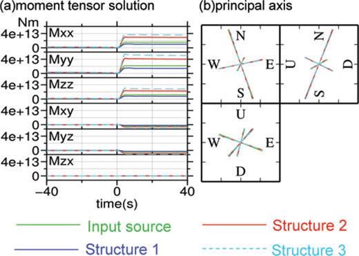
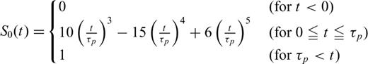
(a) Input source, for numerical tests to estimate model uncertainty caused by uncertainty in velocity structure, is indicated by the green solid lines. The input source is a synchronized expansion of a tensile crack and a cylinder: strike and dip angles of the tensile crack are both 70°, and the symmetry axis of the cylinder is inclined by 30° from vertical and is rotated by 60° from x-axis in horizontal plane in counter-clockwise. The source time function of this input source is eq. (7) with τ_p = 5 s. Blue solid lines are the moment-tensor solution obtained for synthetic seismograms calculated using Structure 1 (see Table 3). Red solid lines are the same for Structure 2 and cyan dashed lines are for Structure 3. (b) Principal axis of the moment-tensor time functions indicated in panel (a), obtained by assuming a time-invariant source mechanism and calculated using the differences between values at t= 20 and −5 s as the amplitudes of the moment-tensors. Line lengths were normalized by the largest principal values. Colours and types of the lines are the same as panel (a), and method of projections is the same as Fig. 11(b).

Open in new tabDownload slide

Table 3

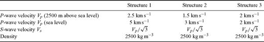
Velocity structure models used to generate the synthetic seismograms for numerical tests, regarding model uncertainty caused by uncertainty of the velocity structure. The structure model used in the inversion is identical to Table 2. P-wave velocities linearly increase with depth.

Open in new tabDownload slide

8.2 Interpretation

The moment-tensor time function (Fig. 11a) is composed of an initial rapid inflation phase and the subsequent gradual deflation phase. Major gradual deflation occurs in a time scale of order of 100 s, which is within the reliable frequency range of the moment-tensor solution (Fig. 11c). Time scale of the initial rapid inflation phase is approximately 10 s, which is near the upper limit of the reliable frequency range (Fig. 11c). However, low-pass filtering with corner frequency of 0.1 Hz to the moment-tensor time functions did not essentially change the time functions, meaning that the initial ∼10-s-long rapid inflation is also reliable. It is not clear whether the moment-tensor finally goes back to the initial value or residual moment-tensor remains, because it does not go back to the initial value within the reliable time scale.

Although the seismic observation can at best infer the forces exerted at the source cavity's wall, and not the source process itself, one of the possible idea of the explanation of the initial rapid inflation phase may be a rapid inflow of gas from deeper reservoir to the VLP-source cavity. The idea is schematically illustrated in Figs 15(a)–(d). In this model, a valve on the path connecting the VLP-source cavity (a tensile crack and a cylinder) and the deeper gas reservoir was initially closed. The pressure in the deeper gas reservoir gradually increases as a result of the gradual accumulation of gas (Fig. 15a), with the accumulation rate being too slow to be detected as a seismic signal. When the pressure in the deeper gas reservoir reaches a critical value, the valve opens and the gas leaks from the deeper reservoir toward the VLP-source cavity (Fig. 15b). The movement of gas somehow accelerates and finally results in a large pressure increase in the VLP-source cavity (Figs 15c–d), generating the initial rapid inflation phase of the VLP pulses. Small oscillations are observed preceding many of the VLP pulses (Fig. 2b), which may be attributed to the first weak leakage of gas.

Figure 15

Schematic source model of VLP pulses at Asama volcano. For explanation, refer to Section 8.2. Although the liquid phase is shown in red in this figure, it may be water as well as magma, and these liquids cannot be distinguished based on seismic analysis. In addition, although the cylinder lies under the crack in this figure, their relative locations are unknown because the inversion was carried out on a point source approximation.

Open in new tabDownload slide

In order to generate a total expansion of the moment-tensor solution, some additional process to disturb decompression of the deeper reservoir is required; otherwise the movement of gas generates a negative moment with the same amplitude at the deeper reservoir, cancelling out the inflation of the VLP-source cavity. Generation of gas in the deeper reservoir, either by boiling of underground water or by exsolution of volatiles from magma, may be a plausible explanation to this. Consider that the deeper reservoir was partially filled with liquid, which may be either water in nearly boiling point or magma with nearly saturated volatiles (Fig. 15a). Because the seismic observation cannot distinguish the species of fluid, we here consider both possibilities (i.e. water and magma) in parallel. When the valve opens and leakage of gas (Fig. 15b) occurs, pressure in the deeper reservoir slightly decreases. In magma case, this pressure decrease promotes volatiles to exsolve from magma, generating additional gases (Figs 15c–d), which compensates for the pressure decrease in the deeper reservoir. In water case, boiling of water may play the same role. In this way the pressure in the deeper reservoir is kept constant, and movement of gas from the deeper reservoir to the VLP-source cavity continues, until the pressure in the VLP-source cavity becomes balanced with that in the deeper reservoir. Speed of this process is controlled by the pressure difference between the VLP-source cavity and the deeper reservoir, together with width of the pathway connecting them and fluid properties.

One of the plausible explanation of the gradual deflation phase (Fig. 11a) may be a gradual escape of gas from the VLP-source cavity to the surface, as is schematically shown in Figs 15(e)–(f). Before 2008, VLP pulses were accompanied by no visible surface activities. Probably the gas had escaped through the whole crater (Fig. 15e) with invisibly long time. After 2009, VLP pulses were followed by distinct slow gas emission events from a vent at the crater bottom (star in Fig. 1), with a time difference of 30–60 min or so. Because these gas emission events started after the end of the dense temporary seismic observation, we cannot perform moment-tensor inversions for the events after 2009. However, high level of waveform similarity (0.96 between event 1 and 2) and similarity in particle-motion pattern (Fig. 7) strongly implies that the source process of VLP pulses after 2009 is not so different from that before 2008. We therefore consider the same inflation process (Figs 15a–d) for VLP pulses in the both span, and consider the deflation process indicated in Fig. 15(f) for the VLPs after 2009. Probably, part of the gas escapes from a pathway, which connect the VLP-source and the vent through which gas can escape relatively easily. However, considering the high level of similarities in seismograms between 2008 and 2009 events, large amount of gas may escape as a similar way to 2008.

8.3 Relationship between the present results and other observations

Fig. 13 summarizes the relationship between the present results, the hypocentre distribution of non-VLP volcanic earthquakes, and surface topography at Asama volcano. Although some uncertainty exists regarding the location, the hypocentre distribution of non-VLP volcanic earthquakes seems to be located northward from the crater centre. The VLP source locations (orange solid quadrangle and red dotted line) lie near the upper limit of the hypocentres of non-VLP volcanic earthquakes, implying a possibility that the conduit itself may be located northward of the crater centre, and that VLP pulses may occur immediately above the magma head.

The orientation of the tensile crack of the ‘tensile crack plus cylinder’ model that generates the VLP pulses (orange solid quadrangle of Fig. 13) is as a first approximation consistent with the regional east–west compressional stress field. As a second approximation, the crack appears to lie along and be sub-parallel to the northern rim of the crater. These characteristics hold even if the true source is located 50 m eastward, with a crack strike being nearly 110°, which is an alternative candidate source mechanism discussed in Section 8.1. Such crack orientation also seems to be consistent with previous studies of fractures at the summit area of volcanoes. For example, Michon et al. (2009) argued that there are three types of fractures near calderas of Piton de la Fournaise, Reunion Island, one of which is concentric fractures. Based on field observations and analogue experiments, Acocella (2007) argued that two ring faults are generated around calderas, one of which is inward-dipping and the other is outward-dipping. The VLP-source crack of the present study appears to be inward-dipping ring fault, as shown in Fig. 13. Given the existence of the crater, the development of an inward-dipping ring fault may readily occur around the summit crater of Asama volcano. However, the existence of an east–west compressional regional stress field means that this ring fault may be weakly developed in the eastern and western parts of the crater. In addition, because the magma conduit is located northward from the crater centre, the ring fault may be weakly developed to the south, meaning that it is prominent in the northern area.

9 Summary

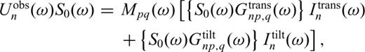
We deployed a dense seismic network at the summit area of Asama volcano, developed an algorithm for moment-tensor inversion without requiring assumptions regarding tilt motions, and applied the algorithm to VLP pulses at Asama volcano. Dense seismic observations revealed particle motions which do not point to a single source location, despite their rectilinearities, suggesting a non-isotropic source mechanism, together with path effect. Moment-tensor inversions for these seismic events yielded ratios of the principal values of moment-tensors of approximately 5: 3: 2, suggesting the synchronized inflation of a tensile crack and cylinder. The strike and dip angle of the tensile crack are both nearly 70° and the symmetry axis of the cylinder is inclined by nearly 30° from the vertical. Moment-tensor time histories are indicative of an initial rapid pressurization and subsequent gradual depressurization at the source region. We considered the inflow and outflow of gas at the VLP-source cavity, generated either by boiling of water or by exsolution of volatiles from magma at deeper gas reservoir. A key contribution of this study to volcano seismology is the consideration of the second term in the braces of the right-hand side of eq. (1), which was realized by combining the FDM code proposed by Ohminato & Chouet (1997) with a Perfect Matched Layer boundary condition developed by Festa & Nielsen (2003) to calculate a long synthetic time trace in the near-field.

Acknowledgments

We are grateful to Assoc. Prof Takao Ohminato for advice, discussions, and for providing computer programs. Ryunosuke Kazahaya and Toshiya Mori offered analyses results of volcanic gas observation, and participated in useful discussions. This paper was improved by discussions with Yosuke Aoki, Mie Ichihara, Hiroshi Aoyama, Satoshi Ide and other participants at seminars held in the Earthquake Research Institute. Professor Philippe Jousset and two other anonymous reviewers also provided constructive comments. The following researchers provided assistance with temporary observations: Takao Ohminato, Atsushi Watanabe, Yosuke Aoki, Mie Ichihara, Jun Oikawa, Takao Koyama, Shingo Watada, Taku Urabe, Hiroshi Tsuji and Etsuro Koyama. MT was partially supported from the Grant-in-Aid for Scientific Research, Japan Society for Promotion of Science (KAKENHI) No. 22540431.

Appendices

Appendix A: Detailed Process of the Observational Plan

The layout of the temporary stations was decided by the following three-step approach.

• 1
  Calculation of synthetic wavefield. First, synthetic wavefield on the free surface were calculated for each of six moment-tensor components at various candidate source locations, using a finite-difference method (FDM) code proposed by Ohminato & Chouet (1997) because the FDM code proposed by Maeda et al. (2011) had not been developed at that time. These two FDM codes share a common algorithm to include arbitrary 3-D topography and structure. The main difference between these codes is that the former uses Clayton's 1st order absorbing boundary condition (Clayton & Engquist 1977), which is not efficient enough to calculate long synthetic waveforms. In addition, the former produces displacement while the latter does velocity; thus the source time function with non-zero DC component such as eq. (7) is not appropriate for the former code. Considering these limitations, a source time function

  

  (A1)

  with τ_p= 0.5 s was adopted. A 10-m-mesh digital elevation model (DEM) and a uniform structure of V_p= 2500 m s⁻¹V_s = V_p/√3 and ρ= 2650 kg m⁻³ was used, which was again a bit different to the structure model used in the inversion because the reliable structure model (Aoki et al. 2009) had not been obtained yet at that time. After trial-and-error simulations to obtain a condition that the waveforms converge to zero before the end of the calculation, without strong contamination by reflected waves from numerical boundaries, 4-s-long synthetic waveforms were calculated using a computational volume of 5 km × 5 km × 2.5 km in size. Grid size was 10 m and time interval was 0.001 s. Calculations were independently conducted for each three single-force and six moment-tensor source mechanisms, located at 2200, 2250 and 2300 m above sea level, below the crater centre; 2300 m above sea level, below 50 and 100 m east, west, north and south of the crater centre; and 2300 m above sea level, below 50 m northeast, northwest, southeast, southwest of the crater centre. These candidate source locations were determined by referring to a previous trial inversion using only permanent stations and a narrow frequency band dominated by translational motions, although it was shallower and nearer to the crater centre than the final inversion result indicated in this paper.
• 2

  Making candidate station layouts. The Fourier amplitude spectra for the obtained synthetic seismograms on the free surface were calculated. There amplitude spectra along the free surface, for 3, 5 and 10 s contents, were plotted for every calculations. Referring to these amplitude spectra patterns, several candidate layouts for the 10 available broad-band seismometers were planned. At this stage, two additional aspects were considered. These were: accessibility to the locations of the candidate stations; and the fact that VLP signals recorded at stations located farther than 1 km from the crater were too weak to be of use in analyses (Fig. 5).

• 3

  Resolution checks. Once a candidate station layout was made, the practical Green's functions (Section 5) for each elementary source mechanisms, stations, and components constituted a data-kernel matrix G. Then a model resolution matrix R=G^−gG was obtained, where G^−g is the generalized inverse of G. The model resolution matrix represents the degree to which the estimated model parameters reflect the ‘true’ model parameters (e.g. Menke 1989); R near to the unit matrix means that the resolution is good. An important point is that R can be constructed purely by the practical Green's functions and thus it does not depend on data; therefore R can be obtained before the real observations, and can be used as a measure of a goodness of the station layout. The difficulty was that R depends not only on candidate station layout but also on candidate source location, the threshold of non-zero singular-value, and the source model (i.e. with single-force or without single-force); thus determination of the ‘best’ station layout was not easy. By carefully comparing the resolution matrices for all the calculations, we decided the layout (Fig. 1), although there were only slight differences (probably within error level) in resolutions for almost all of the tried candidate layouts; therefore it is not clear whether the station layout indicated by Fig. 1 is really ‘best’. At least, the station layout indicated in Fig. 1 resulted in a sufficient resolution for all the moment-tensor components as long as the single-forces were not considered and the singular-values larger than 0.01 times the maximum singular-value were regarded to be non-zero; in this case, for the best-fitting source location of the previous trial inversion, the minimum diagonal component was 0.83. This value is not equivalent to the final inversion because of the difference in source location, and also because the tilt effect was not included and a time-domain inversion algorithm (Ohminato et al. 1998) was used at that time. In the real inversion described in this paper, all the singular-values were non-zero, meaning that the resolution matrices were equal to the unit matrix.

Appendix B: Waveform Similarities Among Events

There are too many VLP events to calculate correlations for all combinations of events, and instead we performed correlation analyses for some selected events. All the following correlations were obtained from vertical seismograms at KAW low-pass-filtered with corner frequency of 0.1 Hz. Seismometer's response was not corrected.

The first analysis was conducted for all the events that occurred within a single day, namely, on August 10, 2008; up to 46 events occurred in this day, including an event which was followed by a very small eruption. Fig. A1(a) shows correlations among them, ordered in time occurred. Among the ₄₆C₂= 1035 pairs of events, only 261 pairs (about 25 per cent) have correlations less than 0.6, showing a high level of waveform similarities among events. There are some dark-coloured lines in Fig. A1(a), indicating that majority of the small correlations occur corresponding to some of the particular events. These events are either noisy or long-duration events; thus similarities among ordinary VLPs are still higher.

Figure A1

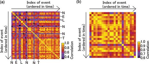
(a) Cross-correlations among VLP events that occurred on 2008 August 10. Events are ordered in time, from top (earliest) to bottom (latest) and from left-hand side (earliest) to right-hand side (latest), and each coloured cells indicate correlations between corresponding events; for example, the colour of a cell in row 1 and column 2 indicates a cross correlation between first and second events in this day. Some events which have relatively lower correlations with majority of events, as is observed by dark-coloured rows and columns. Characters indicated for each of these columns are the possible causes of the low correlations, as follows: ‘N’ is a noisy event, ‘L' is a long-duration event, and ‘T’ is an event composed of two subpulses. ‘E’ is a long (∼50 s) duration event which preceded a very small eruption by 3 min. (b) Cross-correlations among VLP events analysed in this study, as is indicated in Fig. 4. Again, the events are ordered in time, from the VLP at 0:21 on October 1 (left-hand side and top) to the VLP at 7:05 on November 3 (right-hand side and bottom).

Open in new tabDownload slide

The second analysis was conducted for 23 events analysed in this study (Fig. 4). Fig. A1(b) shows correlations among them. Among all the ₂₃C₂= 253 pairs of events, only 31 pairs have cross correlations smaller than 0.8, and only 11 pairs have cross correlations smaller than 0.75, indicating a high level of waveform similarities among events. The smallest correlation is even as high as 0.69, for an event that occurred at 0:21 on October 1 and an event that occurred at 18:01 on October 8. The correlations are better than those among events on August 10, 2008 (Fig. A1a) probably because here we show the correlations among selected events, having high signal-to-noise ratios.

Third, we made correlation analysis for events that occurred in different periods, namely, for three events shown in Fig. 2. Correlations between events shown in Fig. 2 (a) and (b), (a) and (c) and (b) and (c) are 0.91, 0.87, and 0.96, respectively, indicating that event waveform have not essentially changed through this 5-yr-long time span.

References

Author notes