


Summary
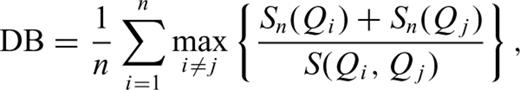
Active volcanoes generate sonic and infrasonic signals, whose investigation provides useful information for both monitoring purposes and the study of the dynamics of explosive phenomena. At Mt. Etna volcano (Italy), a pattern recognition system based on infrasonic waveform features has been developed. First, by a parametric power spectrum method, the features describing and characterizing the infrasound events were extracted: peak frequency and quality factor. Then, together with the peak-to-peak amplitude, these features constituted a 3-D ‘feature space’; by Density-Based Spatial Clustering of Applications with Noise algorithm (DBSCAN) three clusters were recognized inside it. After the clustering process, by using a common location method (semblance method) and additional volcanological information concerning the intensity of the explosive activity, we were able to associate each cluster to a particular source vent and/or a kind of volcanic activity. Finally, for automatic event location, clusters were used to train a model based on Support Vector Machine, calculating optimal hyperplanes able to maximize the margins of separation among the clusters. After the training phase this system automatically allows recognizing the active vent with no location algorithm and by using only a single station.
1 Introduction
Two of the fundamental tasks of volcano monitoring are to follow volcanic activity and promptly recognize any changes. To achieve such goals, reliable field measurements and advanced data analysis methods are required. Different geophysical techniques (i.e. seismology, ground deformation, remote sensing, magnetic and electromagnetic studies, gravimetry) are used to obtain precise measurements of the variations induced by an evolving magmatic system. In recent years, useful information to monitor the explosive activity of volcanoes, as well as to investigate its source processes, have been provided by studying infrasonic signals (e.g. Vergniolle & Brandeis 1994; Ripepe & Marchetti 2002; Cannata et al. 2009a,b; Marchetti et al. 2009). The location of the source of the infrasonic signals, generally coinciding with active vents, is of great importance for volcanic monitoring. Thus, different techniques, generally based on the comparison of the infrasonic signals using cross-correlation or semblance functions, have been developed (e.g. Ripepe & Marchetti 2002; Garces et al. 2003; Johnson 2005; Matoza et al. 2007; Jones et al. 2008; Montalto et al. 2010).
Over the last decades, Mt. Etna volcano (Italy) has been characterized by a remarkable increase in the frequency of short-lived, but violent eruptive episodes at the summit craters. Between 1900 and 1970, about 30 paroxysmal eruptive episodes occurred at the summit craters, while there have been more than 180 since then (Behncke & Neri 2003). The summit area of Mt. Etna is currently characterized by four active craters: Voragine, Bocca Nuova, Southeast Crater and Northeast Crater (hereafter referred to as VOR, BN, SEC and NEC, respectively; see Fig. 1). These craters are characterized by persistent activity that can be of different and sometimes coexistent types: degassing, lava filling or collapses, low rate lava emissions, phreatic, phreato-magmatic or strombolian explosions and lava fountains (e.g. Cannata et al. 2008). At Mt. Etna in 2006, a permanent infrasound network was deployed providing useful information to monitor the explosive activity (Cannata et al. 2009a,b; Di Grazia et al. 2009). Unfortunately, sometimes during the winter season owing to bad weather conditions, the lack of signals from some summit stations prevents applying the aforementioned location algorithms. Here, we propose a new system, based on pattern recognition techniques, able to identify at Mt. Etna the active summit crater from the infrasonic point of view using only the signal recorded by a single station.

Digital elevation model of Mt. Etna with the location of the infrasonic sensors (triangles and squares), composing the permanent infrasound network. The upper right inset shows the distribution of the four summit craters (VOR, Voragine; BN, Bocca Nuova; SEC, Southeast Crater; NEC, Northeast Crater).
2 Infrasound Features at Mt. Etna
Some recent studies have shown that the infrasonic signal at Mt. Etna is generally composed of amplitude transients (named ‘infrasonic events’), characterized by short duration (from 1 to over 10 s), impulsive compression onsets and peaked spectra with most of energy in the frequency range 1–5 Hz (Fig. 2; Gresta et al. 2004; Cannata et al. 2009a,b). Similar features are also observed at several volcanoes, though characterized by different volcanic activity, such as Stromboli (Ripepe et al. 1996), Klyuchevskoj (Firstov & Kravchenko 1996), Sangay (Johnson & Lees 2000), Karymsky (Johnson & Lees 2000), Erebus (Rowe et al. 2000), Arenal (Hagerty et al. 2000) and Tungurahua (Ruiz et al. 2006).
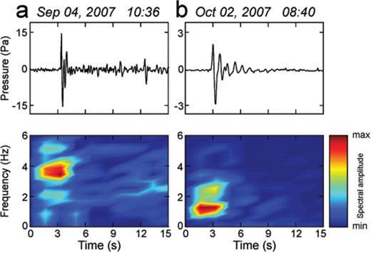
Infrasonic events recorded by EBEL station and corresponding Short Time Fourier Transform, obtained by using 2.56-s long windows overlapped by 1.28 s. The event in (a) is a typical ‘SEC event’, the one in (b) a typical ‘NEC event’.
Since the deployment of the infrasound permanent network at Mt. Etna in 2006, two summit craters have been recognized as active from the infrasonic point of view: SEC and NEC (Cannata et al. 2009a,b). The former has been characterized by sporadic explosive activity with different intensity, from ash emission to lava fountaining, while the latter mainly by degassing. According to Cannata . (2009a,b), these craters generate infrasound signals with different spectral features and duration: ‘SEC events’, showing a duration of about 2 s, dominant frequency mainly higher than 2.5 Hz and higher peak-to-peak amplitude than the NEC events (Fig. 2a); ‘NEC events’, lasting up to 10 s and characterized by dominant frequency generally lower than 2.5 Hz (Fig. 2b).
3 Data Acquisition and Infrasound Signal Characterization
In the following subsections (i) data acquisition and event detection, (ii) features extraction and (iii) the semblance algorithm are briefly described.
3.1 Data acquisition and event detection
Since 2006, the permanent infrasound network run by Istituto Nazionale di Geofisica e Vulcanologia, Section of Catania, has been composed of a number of stations ranging from one to eight depending on the considered period, located at distances ranging between 1.5 and 7 km from the centre of the summit area (Fig. 1). Today, some stations are equipped with Monacor condenser microphones MC-2005, with a sensitivity of 80 mV Pa−1 in the 1–20 Hz infrasonic band, while others with GRASS 40AN microphone with a flat response with sensitivity of 50 mV Pa−1 in the frequency range 0.3–20000 Hz. The infrasonic signals are transmitted in real-time by means of radio link to the data acquisition centre in Catania where they are acquired at a sampling rate of 100 Hz.
At Mt. Etna we use EBEL as reference station, because it generally shows a very good signal-to-noise ratio and, unlike the other summit stations, its maintenance is generally feasible even during the winter season. Once the infrasound signal is recorded, the signal portions of interest, that are the infrasonic events, have to be extracted. Then, the root mean square (rms) envelope of the infrasonic recordings is calculated by a moving window of fixed length. Successively, we calculate the percentile envelope on moving windows of rms envelope. For a given time-series, the pth percentile can be defined as the value such that at most (100 ×p) per cent of the measurements are less than this value and 100(1 –p) per cent are greater. In light of this, the estimation of percentile enables us to efficiently detect amplitude transients and estimate background signal level. The percentage threshold should be chosen on the basis of both the amount of transients in the signal that have to be included or excluded in our calculations and the signal-to-noise ratio. The performance of this method was compared with the short time average/long time average (STA/LTA) technique (e.g. Withers 1997; Withers et al. 1998). The lengths of short and long windows, mainly depending on the frequency content of the investigated signal, were fixed respectively to 2.5 and 12.5 times the dominant period of the signal (equal to roughly 0.3 s), considered a reasonable compromise between sensitivity and noise reduction (Withers 1997), and the detection threshold to 1.7. As shown in Fig. 3, the trigger results obtained by the two methods were similar; nevertheless, the technique based on percentile was also able to detect transients very close to each other.
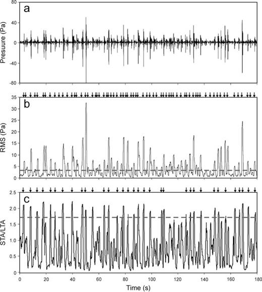
(a) Three-minute long infrasound signal recorded by EBEL station, (b) corresponding rms envelope (black line) calculated by using a moving window of 0.7 s and (c) STA/LTA values. The horizontal grey dashed line in (b) indicates the detection threshold calculated by a percentile value of 5 multiplied by 5. The horizontal grey dashed line in (c) indicates the detection threshold fixed at 1.7. The arrows at top of (b,c) indicate the onset time of the detected events.
3.2 Infrasonic signal features extraction

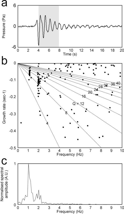
(a) Infrasound event recorded by EBEL station, and corresponding (b) frequency-growth rate plot (AR order 2–60) and (c) amplitude spectrum. The grey area in (a) represents the window used to calculate the frequency-growth rate plot in (b). The dashed lines in (b) represent lines along which the quality factor (Q) is constant. Clusters of points in (b) indicate dominant spectral components of the signal; scattered points represent noise.
Further, in addition to frequency and quality factor, the third feature used to characterize the infrasound events is the peak-to-peak amplitude, depending on both distance source-station and energy of the infrasonic source.
3.3 Semblance algorithm
The location of the source of the infrasonic events, generally coinciding with active vents, is of great importance for volcanic monitoring. Therefore, different location techniques, generally based on grid searching procedures, were developed (e.g. Ripepe & Marchetti 2002; Jones et al. 2008; Johnson et al. 2010; Montalto et al. 2010). The semblance technique is based on the semblance function that is a measure of the similarity of multichannel data (Neidell & Taner 1971). For infrasonic events this method applies a 2-D grid searching procedure over a surface covering the summit area and coinciding with the topographic surface. The infrasonic source is assumed to be in each node of the grid, and for each node the theoretical traveltimes at the sensors are first calculated. Then, infrasonic signals at different stations are delayed and compared by the semblance function. Finally, the source is located in the node where the delayed signals show the largest semblance value. Therefore, the semblance function is assumed representative of the probability that a node has to be the source location (further details about the method are reported in Montalto et al. 2010). In Fig. 5 two examples of infrasound location are reported for a SEC event and a NEC event.
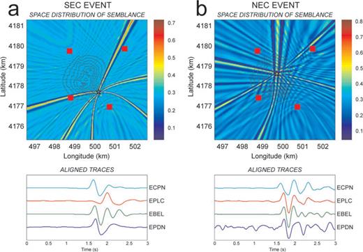
Examples of space distribution of semblance values, calculated by locating two infrasonic events at Mt. Etna, and corresponding infrasonic signals at four different stations shifted by the time delay that allows obtaining the maximum semblance. The red squares and stars in the top plot indicate four station sites and the nodes with the maximum semblance value, respectively. The black lines in the top plot are the altitude contour lines from 3 to 3.3 km a.s.l.
4 Pattern Recognition Techniques
Automatic extraction, recognition, description and classification of patterns extracted from images and signals are important tasks in several scientific disciplines. For instance, several studies based on pattern recognition (hereafter referred to as PR) techniques have been performed on seismo-volcanic signal analysis (e.g. Ohrnberger 2001; Kohler et al. 2009). The main aspect of PR is the definition of a set of peculiar features or descriptive elements of the analysed objects. Given a pattern, the recognition process consists of one of the following tasks: (i) supervised classification in which objects are classified on the basis of inference rules acting on a set of knowledge patterns (Joswig 1990); (ii) clustering that is the process of grouping sets of objects into classes called clusters with no a priori knowledge.
In the first case, the classifier design can be implemented by several techniques, implying the definition of a metric based on template matching or the minimum distance between pattern and class prototype. Other classification techniques are based on geometric approaches. These kinds of classifiers are based on a training procedure that minimizes an error (such as the mean square error, MSE) computed comparing classification output and target value. A powerful method in classifier design is the Support Vector Machine (SVM) introduced by Vapnik (1998). This algorithm is different from other hyperplane-based classifiers such as single layer perceptron. The problem of estimating hyperplane that separates two classes is not unique. The SVM algorithm is able to find the optimal hyperplane that separates the classes.
Another important task in PR is the clustering problem that, as aforementioned, is the process of grouping data without any a priori information. Objects belonging to the same cluster will be more similar than objects belonging to different clusters with respect to some given similarity measures. Many clustering methods exist in literature (Berkhin 2002). These can be broadly divided into hierarchical and partitioning. Hierarchical algorithms gradually (dis)assemble objects into clusters. On the other hand, partitioning algorithms learn clusters directly, trying to discover clusters either by iteratively relocating points between subsets or by identifying areas heavily populated with data. This second type of partitioning algorithms attempts to discover dense connected components of data. Examples of algorithms belonging to such a category are: DBSCAN, OPTICS and DENCLUE (Berkhin 2002). The system proposed in this work uses both clustering and classification algorithms to develop an automatic procedure able to discover and classify clusters in a given feature space. The algorithm chosen for pattern clustering and classification are DBSCAN and SVM, respectively.
4.1 Clustering algorithm based on DBSCAN
Density-Based Spatial Clustering of Applications with Noise (DBSCAN; Ester et al. 1996) is a density-based clustering algorithm able to discover clusters of arbitrary shape in spatial databases with noise. Clusters are defined as maximal sets of density-connected points. Usually DBSCAN runs on data sets drawn from multidimensional or metric spaces and uses a distance function to compare objects. Given a data set D of objects, DBSCAN makes use of the following structures and definitions (Ester et al. 1996): (i) ɛ-neighbourhood, (ii) core point, (iii) directly density-reachable, (iv) density-reachable and (v) density-connected. The ɛ-neighbourhood of a point p, denoted by Nɛ(p), is a subset of points q in D, such that a distance measure dist(p,q) (such as the Euclidean distance) is lower than ɛ. The point p is called core point or core object if its ɛ-neighbourhood has cardinality above a minimum threshold called MinPts. Each point q which lies in the ɛ-neighbourhood of a point p is called directly density-reachable from p (Fig. 6a). A point q is density-reachable from a point p with respect to ɛ and MinPts if there is a chain of points q1,…, qn such that q1=p, qn= q and qi+1 is directly density-reachable from qi for each i (Fig. 6b). A point q is density-connected to a point p with respect to ɛ and MinPts if there is a point o such that both p and q are density reachable from o with respect to ɛ and MinPts (Fig. 6c).
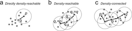
Examples of (a) directly density-reachable, (b) density-reachable and (c) density-connected in density-based clustering. Suppose MinPts = 3. Grey and black dots indicate the points to group into clusters, black circles delineate the area of radius ɛ around black dots, the arrow denotes the relation of direct density-reachability. In (a) dot p is the so-called core point, while q is directly density-reachable from p. In (b) dot q is density-reachable from p. In (c) dot q is density-connected to p and o is a point such that both p and q are density reachable from o (for details see Section 4.1).
Given D, ɛ and MinPts as input parameters, DBSCAN clusters D by checking the ɛ-neighbourhood of each object in D. If the ɛ-neighbourhood of an object p contains more than MinPts, a new cluster with p as core object is created. DBSCAN iteratively collects directly density-reachable objects from these core objects. The process terminates when no new objects can be added to any cluster. In such a case, the algorithm will return the set of clusters and a special cluster containing outliers.
4.2 Features classification using SVM
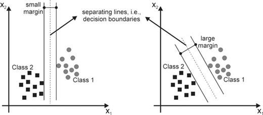
Two-feature planes each of which with two classes of data (black squares and grey circles) and a separating line (dashed lines): the left one shows a small margin between clusters, the right one a larger margin (redrawn from Kecman 2001).
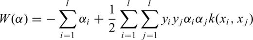
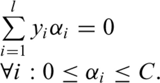
The kernel for linear boundary function is xiyi, a scalar product of two data points. The non-linear transformation of the feature space is performed by replacing k(xi, yi) with an advanced kernel ϕ, such as polynomial kernel (xTxi+ 1)p or a radial basis function kernel  . The use of an advanced kernel is an attractive computational shortcut, which avoids the expensive creation of a complicated feature space. An advanced kernel is a function that operates on the input data but has the effect of computing the scalar product of their images in a usually much higher-dimensional feature space (or even an infinite-dimensional space), which allows one to work implicitly with hyperplanes in such highly complex spaces (Fig. 8). The extension of SVM to multiclass problems can be performed using two different methods called one-against-one and one-against-all. The former constructs k(k−1)/2 classifier where each one is trained on data from two classes. The latter constructs k SVM classifier. In this last case, the ith SVM is trained using all training patterns belonging to ith class with positive labels and the other with negative labels. A point is assigned to the class for which the distance from margin is maximal. Finally, the output of one-against-all method is the class that corresponds to SVM with highest output value (Weston & Watkins 1999; Hsu & Lin 2002).
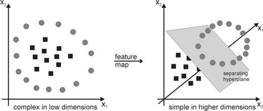
Two classes of data in the original 2-D space (left) and in a higher-dimensional feature space (right).
4.3 Learning phase
In the proposed system, the learning phase merges together results of clustering and classification analysis (Fig. 9). The techniques described in Section 4.1 and 4.2 are applied on infrasound event features together with geophysical information used to ‘labeL' the recognized clusters. About 665 events, recorded during 2007 September–November at EBEL station, were detected and filtered in frequency range 0.5–5 Hz. The feature extraction from the detected events was performed by Sompi method (Section 3.2) using 2-s long windows of infrasonic signal recorded at EBEL station and AR order equal to two. The sharply monochromatic nature of the investigated signals justifies the choice of this low order (Lesage 2008). Frequency and quality factor of the events, together with peak-to-peak amplitude, constituted the feature space and are plotted in Fig. 10. Then, to discover clusters in this space, ‘data clustering’ techniques based on DBSCAN algorithm (Section 4.1) were applied. Using such an algorithm we found three main clusters (called cluster 1, 2 and 3) and other outlier points that can be considered as noise (Fig. 11). Points belonging to each cluster are related to infrasonic events that were located using Semblance location method (Section 3.3). In accordance with Cannata et al. (2009b), during 2007 September–November, two infrasonic sources were found, NEC and SEC. In particular, a cluster was composed of events generated by NEC (cluster 1) and the other two by SEC. Such last two clusters were related to different kinds of explosive activity at SEC. In particular, the events belonging to cluster 3 were coincident with ‘more visible’ explosions, characterized by a relevant presence of ash, whereas the events of cluster 2 were hardly visible in the monitoring video-camera recordings (Cannata et al. 2009b). Features clustering together with labels provide the patterns for SVM learning process.
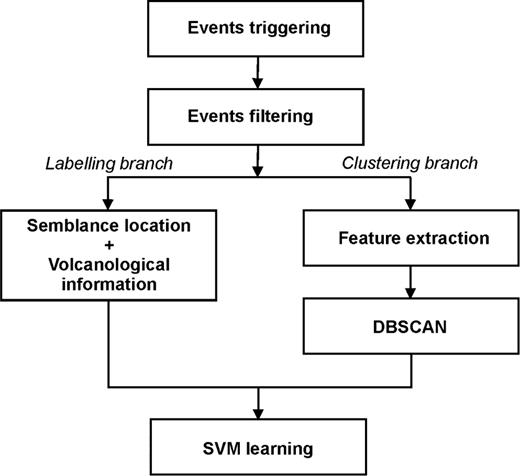
Scheme of the learning system.
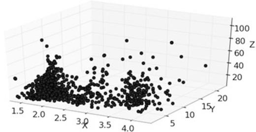
Feature space with frequency, quality factor and peak-to-peak amplitude of the infrasound events recorded at EBEL station during 2007 September–November 2007.
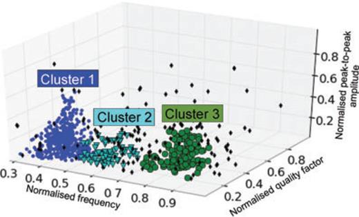
Clustering of the feature space reported in Fig. 10. The clusters are indicated with blue (cluster 1) and green circles (cluster 3) and light green triangles (cluster 2), the outliers with black diamonds.
As mentioned in Section 4.2, optimization of parameters C (regularization parameter) and σ (radial basis function kernel parameter) is a key step in SVM learning because their values determine classification performance (Devos et al. 2009). As a consequence, model selection is applied with the aim of finding the best pair of parameters C and σ that minimizes the error rate estimated as the ratio between misclassified and hit patterns. These parameters can be chosen using a cross-validation (CV) approach (Hastie et al. 2002), which is a statistical method for learning algorithms evaluation and model selection. In particular, in K-fold CV the available data set is partitioned into K subsets or ‘folds’: K–1 folds are used for SVM learning purpose, and the remaining fold for model validation (Fig. 12). Thus, K iteration of learning and validation are performed and for each ith iteration the training process is carried out using K−1 folds and the ith fold for validation (Fig. 12). All SVM training algorithms are computed using one-against-all method (see Section 4.2). Since we worked on a small data set, a simple exhaustive grid search can be performed (Hsu et al. 2007). In particular, C was systematically changed in the range [1–100] with a step of 10, σ in the range [0.1–10] with a step of 0.5 and a K-fold CV with K= 10 was used. The entire procedure can be summarized as follows (Fig. 13): (1) a grid value of C and σ is defined; (2) for each pair of C and σ values, a mean error rate is computed averaging the error rate values obtained by the K SVM models; (3) the pair of C and σ with the minimum error rate is selected; (4) such a pair is used to train the final SVM model with the whole data set, comprising all the K folds. Here, the best parameter values were C = 1 and σ= 0.1, for which mean CV error minimized to 0.6 per cent.
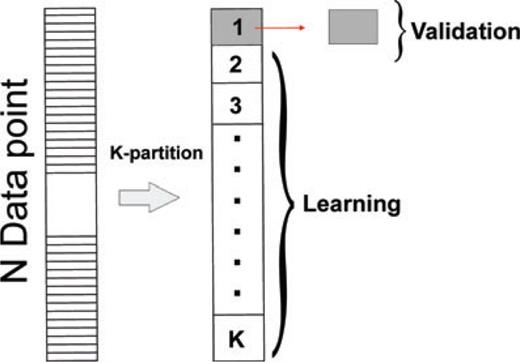
Basic scheme of K-Fold Cross-validation (see Section 4.3 for details).
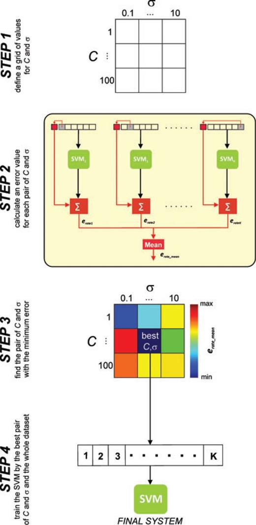
Best SVM model selection using K-Fold Cross-validation (see Section 4.3 for details).
4.4 Testing phase and final system
To verify the system, the trained SVM is tested by classifying new unknown infrasonic events and then assigning them to their source crater. The reliability is verified using events not analysed during the previous learning phase (Section 4.3). To this end, a new test data set of about 610 events, recorded during 2 months, 2007 August and December, was used and labelled by location algorithm based on semblance method (Section 3.3). Moreover, the events belonging to cluster 2 and cluster 3 were labelled using information related to the intensity of the explosive activity (Cannata et al. 2009b). The quality of classification is quantified using confusion matrix (Table 1), where each column represents the instances in the predicted class (based on the SVM model), while each row represents the instances in the actual class (based on the previously attributed labels). Thus, the entries on the diagonal count the events in which prediction agrees with known labels, whereas the other entries the misclassified events. 63 elements were wrong assigned, providing an error rate of about 11.97 per cent. Misclassifications were mostly concentrated in the second and third classes that are related to the two different explosion activities of SEC crater. Indeed, such a distinction is qualitative and not clearcut, hence many halfway events can be misclassified. If we do not take into account the distinction between clusters 2 and 3, and consider them as a single cluster, the error decreases to 5.25 per cent.
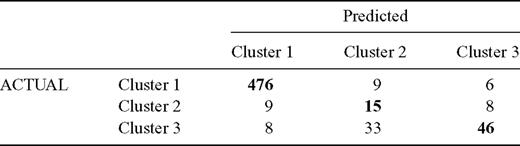
Confusion matrix calculated in the testing phase. Each column represents the instances in the predicted class (based on the SVM model), while each row represents the instances in the actual class (based on the previously attributed labels). Thus, the entries on the diagonal (bold numbers) count the events in which prediction agrees with known labels, whereas the other entries the misclassified events.
Finally, the proposed system can be summarized as follows (Fig. 14): (i) triggering procedures is performed on buffer of acquired signal; (ii) then, if events are found, the system evaluates whether there is a sufficient number of stations for semblance location algorithm; (iii) if the number of stations is not sufficient, alternative ‘single station’ location is performed by extracting signal features and classifying them using the trained SVM. It is also worth noting that SVM classifier is also applied offline on localizable events to evaluate its performance in distinguishing NEC events (cluster 1) from SEC events (clusters 2 and 3). In this case, events belonging to clusters 2 and 3 are simply considered SEC events and then labelled based on the source vent, with no further distinction depending on the type of explosive activity. This task is carried out by comparing the results of the classifier with the location parameters provided by the semblance algorithm. By the inspection of the obtained error rate, a new clustering execution is necessary when classification of new signals is not aligned with that of infrasonic network classifier. This may be caused by the creation of a new active vent or by the changing activity of a pre-existing vent; in such a case the system must be updated.

Flow chart of the proposed location system.
5 Conclusions
At active volcanoes the detection and location of explosive activity is generally obtained by videocameras and thermal sensors (Harris et al. 1997; Bertagnini et al. 1999). However, the efficiency of such instruments is severely reduced or inhibited in case of poor visibility caused by clouds or gas plumes. In these cases, the detection and characterization of explosive activity by infrasound is very useful (e.g. Cannata et al. 2009a) and some techniques, based on infrasound signals recorded by arrays or networks, were developed to locate the source of this signal and therefore the active vent (e.g. Ripepe & Marchetti 2002). All these techniques require that most of the stations work properly and that the noise level is low. Unfortunately, sometimes during winter season, because of bad weather conditions, the possible lack of signals from some summit stations prevents applying the aforementioned standard location algorithms. At Mt. Etna, the events at a single vent for a certain type of activity maintain their features stable over time (Cannata et al. 2009b). Therefore, once the link between event characteristics and vent is known we can understand which crater is active and which volcanic activity is going on by simply extracting the features of the infrasonic signal at a single station (dominant frequency, quality factor and peak-to-peak amplitude). In the light of this, a system, whose learning phase is based on clustering (DBSCAN) and classification techniques (SVM), together with geophysical information, was developed. After the training phase this system automatically allows recognizing the active vent, with no location algorithm and by using only a single station with a success of ∼95 per cent.
It should be noted, however, that in a volcano as Etna, characterized by almost continuous eruptive activity with different styles and topographical variations of the summit area, the vent geometry can change and consequently also the infrasound spectral features. Therefore, spectral characterization and source location must be considered complementary, especially when long lasting periods are investigated.
Acknowledgments
We are grateful to the Editor Matthias Hort and two anonymous reviewers for their constructive criticism. We thank Stephen Conway for revising and improving the English text. Work partly performed with grants of the ‘Flank project’ (INGV-DPC 2007–2009).
Appendix
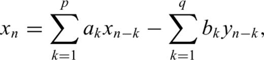
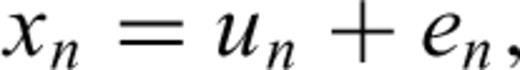
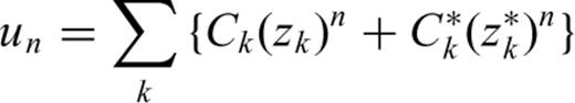
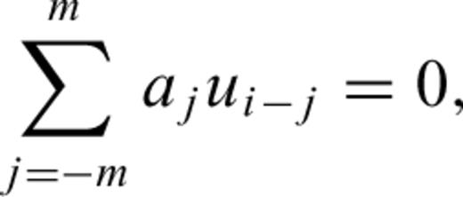
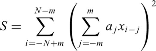
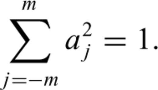
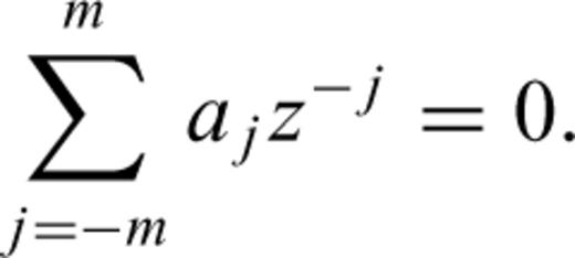
Appendix: SOMPI Method

References
