The use of gravimetric data from GRACE mission in the understanding of polar motion variations

Summary

1 Introduction

The primary cause of the Earth's polar motion is the mass transport within the geophysical fluids layers. In the terrestrial frame Oxyz (where the Oz axis intersects the crust at the geographic North Pole and Ox axis defining the primary terrestrial meridian), off-diagonal inertia moments (I_xz, I_yz) of the Earth undergo changes in mass distribution. In addition, relative motion also takes place. Thus, a time-variable equatorial angular momentum is created, constituted by a ‘mass term’, where represents the terrestrial components of the Earth's angular velocity vector, and a relative angular momentum (‘motion term’). Because of angular momentum conservation principle, that increment is balanced by motion of the rotation pole with respect to the crust. By estimation of the mass term and relative angular momentum, it is possible to provide an estimation of the excitation of polar motion. Until now, those quantities have been partially determined with observations and models of the atmosphere and the ocean, which are known to be the main source of angular momentum changes at seasonal and sub-seasonal scales. The assimilation of various meteorological observations into Global Circulation Model permits to estimate the atmospheric angular momentum (AAM) routinely from pressure and wind fields. The determination of the oceanic angular momentum (OAM) is more difficult because oceanic observations are not largely widespread. Whereas AAM explains 90 per cent of the length of day (LOD)variations at seasonal and sub-seasonal scales (Eubanks 1993), combined AAM and OAM series fit up to 80 per cent of the excitation found in polar motion at these periods (Nastula & Ponte 1998; Gross et al. 2003). That may be due to the defect of OAM model or to the neglect of some other geophysical excitation, like the one linked to hydrological processes. The advent of the Gravity Recovery and Climate Experiment (GRACE) mission related to the entire mass distribution of Earth has shed light on the polar motion excitation. Variability of the gravity field is now monitored with unprecedented accuracy and spatial resolution since 2002 March. The inertia moments (I_xz, I_yz) are directly related to the spherical harmonics coefficients C₂₁ and S₂₁ of the geopotential. We can assume that GRACE mission permits the determination of the equatorial part of the variable mass term, independent of any geophysical model. The GRACE mass term has to be compared with the excitation derived from in the observed polar motion and this at seasonal and sub-seasonal timescales. We now have at hand 4 yr of observations. Our objective is to understand to which extent mass redistribution observed by GRACE is consistent with Earth's rotation observations.

Such a study already initiated by Chen & Wilson (2003), Chen et al. (2004) and revisited by Nastula et al. (2007) for the previous GRACE products releases is extended here for the most recent release. Recent studies done by Chen & Wilson (2008) and Gross et al. (2009) for the GRACE Release 4 (RL04) processing by Center for Space Research (CSR), Austin, USA, are here completed using the analysis of GRACE data carried out by four centres: CSR, GeoForschungsZentrum (GFZ), Postdam, Germany; Jet Propulsion Laboratory (JPL), Pasadena, USA, and Groupe de Recherche en Géodésie Spatiale (GRGS), Toulouse, France. GRGS solution is different from the other ones since it is obtained by combining GRACE and Laser Geodynamics Satellites (LAGEOS) data (Biancale et al. 2007). LAGEOS data provide over 90 per cent of the information on the coefficient C₂₀ of the gravity field, whereas GRACE data provide nearly 100 per cent of the information on all other harmonic coefficients.

Each centre provides updated solutions in several releases. The time span is extended, and the data processing, in particular the models, is revised. Recently CSR, GFZ and JPL have updated their products in the GRACE ‘Release 04’. Our investigation uses this latest version of the gravity field solution in the form of normalized spherical harmonic coefficients for each centre. It reveals a better agreement with polar motion observations than what was obtained by Nastula et al. (2007), especially for the CSR solution.

The recent GRACE data are more accurate, which may help to improve geophysical models. This in turn may help to develop more accurate releases of the gravity fields. The semi-annual and ter-annual signals as well as seismic and tectonic events should be better determined from future GRACE data.

It is noted that C₂₀ coefficient obtained by GRACE is still contaminated by ocean tide model errors (Chen & Wilson 2008); therefore our investigation is limited to polar motion excitation. It would be possible to make a more accurate study on C₂₀ coefficient, which is linked to (LOD; Chen et al. 2004), using Satellite Laser Ranging (SLR) data (Bourda 2008) or the GRGS solution based on the combined LAGEOS/GRACE data.

2 Polar Motion Excitation

2.1 Polar motion excitation from gravity field

Polar motion excitation is deduced from the relation between normalized spherical harmonic coefficients of the gravity field and off-diagonal inertia moments of the Earth in the terrestrial frame. We have used the Chen et al. (2004) formulation for computing excitation functions from the different gravity field solutions (CSR, GFZ, JPL and GRGS):

1

2

where M and R are, respectively, the mass and mean radius of the Earth, C and A are the principal inertia moments of the Earth and k′₂ = −0.310 is the degree 2 load Love number. In our study, these excitation functions are called gravimetric-based excitations functions.

For each centre, the and are corrected from solid Earth tides (McCarthy & Petit 2004), oceanic tides using the FES2004 model (LeProvost et al. 1994), pole tide (McCarthy & Petit 2004), ocean pole tide (Desai 2002), non-tidal atmospheric and oceanic effects using European Center for Medium-range Weather Forecasts (ECMWF) model and Ocean Model for Circulation Tides (OMCT) baroclinic model, respectively (Flechtner 2007), except for the GRGS, which uses a barotropic oceanic model Modèle 2D d'Ondes de Gravité (MOG2D; Carrère & Lyard 2003). For C₂₁ and S₂₁ estimated by the GRGS, LAGEOS is a minor contributor. The relative percentage of participation of the normal equation diagonal to accumulation is between 0 and 5 per cent (Lemoine, private communication, 2008), and it indicates that nearly 100 per cent of the information is due to GRACE data.

The non-tidal models have to be added back, to compare with polar motion excitation deduced from Earth rotation observations.

2.2 Geophysical fluids models of the mass term

We consider separately each of the three geophysical fluids: atmosphere; ocean and the hydrological reservoirs. For the atmospheric excitations, we use a 6-hr excitation series based on the National Center for Environmental Prediction/National Center for Atmospheric Research (NCEP/NCAR) reanalysis (Salstein et al. 1993); the mass excitation accounts for the inverted barometer response of the ocean to the overlying atmospheric pressure. It is provided by the Special Bureau for Atmosphere (SBA) of the International Earth Rotation and Reference System Service (IERS).

For assessing the impact of the geophysical fluids models in our results, we have selected two different OAM series. The first one is computed from the estimates of an ocean model integrated at JPL and provided by the Special Bureau for the Oceans (SBO) of the IERS (Gross et al. 2003). The second one is an experimental series provided to us by R. M. Ponte at Atmospheric and Environmental Research (AER), Inc. It is produced as part of the Estimating the Circulation and Climate of the Ocean—Global Ocean Data Assimilation Experiment (ECCO—GODAE) project (Heimbach et al. 2006; Wunsch & Heimbach 2007; see also http://www.ecco-group.org/). Both oceanic computations are based on the Massachusetts Institute of Technology (MIT), USA, model and are forced by wind stress, heat and freshwater fluxes from the atmospheric reanalysis from NCEP/NCAR. The main difference is that ECCO—GODAE solutions are constrained to fit as much of the global ocean observational data sets as is practicable. A list of the major data sets used to constrain the ECCO—GODAE estimates is given by Wunsch & Heimbach (2006). Other significant difference is the space resolution considered in the models. JPL model use 46 levels of vertical resolution and horizontal resolution of (1/3)° at equator to 1° at high latitudes × 1° longitude. In the case of ECCO—GODAE estimates, the model vertical resolution consists in 23 levels with 1° horizontal resolution in latitude and longitude.

Several models of latitude-longitude grids providing the charge of continental water by surface unit at monthly interval are available for the period 2002–2007. By integrating the grids of water thickness of the National Oceanic and Atmospheric Association's (NOAA's) Climate Prediction Center (CPC) model, we reconstructed the series of the hydrological excitation function or hydrological angular momentum (HAM) reduced to its mass term.

2.3 Geodetic polar motion excitation

The IERS provides combined time-series C04 of the Earth Orientation Parameters (EOP) at daily intervals (Gambis 2004; Bizouard & Gambis 2007). In particular, the pole coordinates x and y allows to compute the geodetic polar motion excitation functions, labelled ‘G’, according to

3

where p = x− i y is the complex pole coordinate and σ_c is the Chandler frequency (2π/433 rad d⁻¹), with an quality factor of 175 (Chen et al. 2004). For computation of the polar motion derivative with respect to time, t, we used the simple approximation

where Δt is the sampling of the series, here 1 d. Error in polar motion is about 50 μas. For periods longer than 2 months (the Nyquist period of GRACE determination), the error on G remains below 1 mas, as it can be shown by considering the Fourier transform of G(t).

Because gravimetric based excitation computed from GRACE solutions only reflects the mass redistribution, we need to remove the motion part from the geodetic excitation associated with the atmospheric winds and ocean currents. NCEP/NCAR reanalysis wind term, denoted by ‘W’, is provided by the SBA, and for the oceanic current term estimation, denoted by ‘C’, we use two different series: the ECCO_kf049f (Gross et al. 2003) available from the SBO and an experimental series provided by Rui Ponte (private communication, 2007) from ECCO—GODAE project computation, to study the influence of the models.

2.4 Sampling and filtering of the excitation series

Time-series of the CSR, GFZ and JPL solutions present a common sampling of about 30 d, whereas the GRGS solution is given at approximately 10 d intervals. On the other hand, geophysical and geodetic excitation functions of polar motion are given at 6 hr up to 1 month. Applying Vondrak smoothing (Vondrak 1969, 1977), which transmits 95 per cent of the signal at 90 d (1 per cent transmitted at 17 d, 55 per cent transmitted at 60 d), we make the GRGS, CSR, GFZ and JPL GRACE solutions, geodetic series and geophysical series spectrally consistent. All these solutions are then interpolated for common dates at 30 d intervals.

Due to the limited number of data points (39), the correlation criteria must be interpreted with care. The Student t test is used for estimating the 90 per cent significance level of correlation coefficient for 39 points, and the result is 0.208. The standard error of the difference between two values of correlation estimated as , where N₁ and N₂ represent the number of independent points in each series; for N₁ = N₂ = 39, value is 0.236. In this way, we have fixed the significance level for all correlations that will be given in the following paragraphs.

Means and linear trends are removed from all time-series.

3 Comparison of Mass Terms Excitation

The gravimetric-based excitation functions of polar motion are shown in Fig. 1. The calibrated errors are associated with the GFZ fields, which provide an approximate lower limit on the uncertainty of the gravimetric based series. They are typically smaller than the residuals between various gravimetric excitation functions (Fig. 2). Apart from two outliers (e.g. beginning of 2004, the end of 2005 for χ₁ and the beginning of 2006 for χ₂), the residuals between the gravimetric based excitation estimated from CSR, GFZ and JPL solutions are generally smaller than 20 mas peak to peak.

Figure 1.

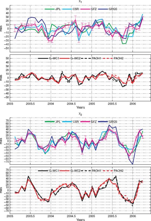
Mass part of excitation functions χ₁ (top panel) and χ₂ (bottom panel) from ‘gravity’ field variations, from ‘geodetic’ observations and from geophysical fluids models. G-WC1, geodetic mass term estimated using the wind term from NCEP/NCAR reanalysis and the current term from SBO series; G-WC2, geodetic mass term estimated using the wind term from NCEP/NCAR reanalysis and the current term from ECCO-GODAE series; CSR, GFZ, JPL, GRGS, ‘gravimetric’ excitations; PAOH1, atmospheric (NCEP/NCAR) + oceanic (SBO) + hydrological (CPC) pressure term; PAOH2, atmospheric (NCEP/NCAR) + oceanic (ECCO-GODAE) + hydrological (CPC) pressure term.

Open in new tabDownload slide

Figure 2.

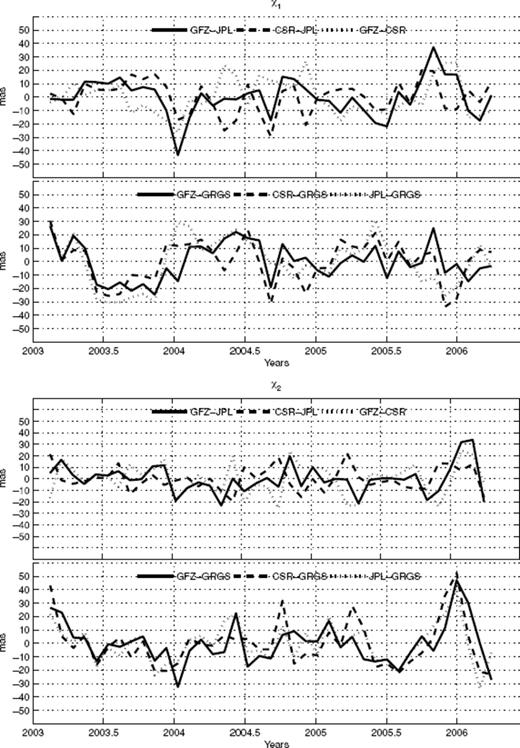
Residuals between mass part of the various excitation functions χ₁ (top panel) and χ₂ (bottom panel) from ‘gravity’ field variations (CSR, GFZ, JPL, GRGS).

Open in new tabDownload slide

Residuals between the CSR, GFZ and JPL gravimetric based excitation and the GRGS gravimetric-based excitation functions are also in the range of 20 mas but with distinct seasonal signal. The analysis of correlation for all the gravimetric-based excitations series are shown in Table 1. Correlation coefficient are computed separately for χ₁ and χ₂ and for the complex combination χ₁ + iχ₂.

Table 1.

The quotient defined as var(X−Y)/[var(X)+var(Y)], where var denotes variance and (X,Y) is the various pairs of ‘gravimetric’ (CSR, GFZ, JPL, GRGS) χ₁ and χ₂ series, represents a crude mesure of noise in the GRACE series; correlation coefficients are computed separately for the χ₁ and χ₂ components and for the complex combination χ₁ + iχ₂ expressed by its magnitude and phase

Open in new tabDownload slide

Despite the spread of the amplitudes, the gravimetric excitation functions are significantly correlated, particularly for the χ₂ components. There is a lower correlation between χ₁ components than between the χ₂ components, may be related to different data processing, which seems to particularly affect the C₂₁ estimate. Additionally, we estimated a rough measure of the noise in all the gravimetric based excitation series as the ratio of the variance between two series to the sum of their variance (see Table 1). The results confirmed the correlation analysis and the better agreement among the χ₂ series than among the χ₁ series. Considering the excitation vector in the complex case, we find that the correlation between the CSR and JPL is maximal but not significantly different from the others. The phase differences are the largest for the GRGS/JPL (−16°) whereas the smallest (1°) corresponds to GRGS/GFZ. In Fig. 1, we compare all the ‘gravity’ excitation functions to the geodetic equatorial excitation functions from which winds (NCEP) and oceanic currents are removed (two cases: OAM series from SBO and the experimental series of ECCO—GODAE project), labelled ‘G—WC’. This comparison is completed by adding the modelled geophysical mass term: containing atmospheric pressure (NCEP/NCAR), hydrological mass term (CPC) and oceanic pressure either using the SBO series (PAOH1) or the ECCO—GODAE experimental series (PAOH2). From Fig. 1, we see that the impact of different ocean current computation on resulting mass term is smaller than 5 mas. The impact of the different oceanic pressure in the geophysical mass term (PAOH) is larger but also relatively small compared with estimated values of excitations and remains largely below 10 mas. Consistent with the visible inference from Fig. 1, there is generally a significant correlation for the component χ₂ (0.8–0.9; Table 2). In the case of χ₁ function, which is mainly associated with mass transport over oceanic regions, correlation drops to 0.4–0.8.

Table 2.

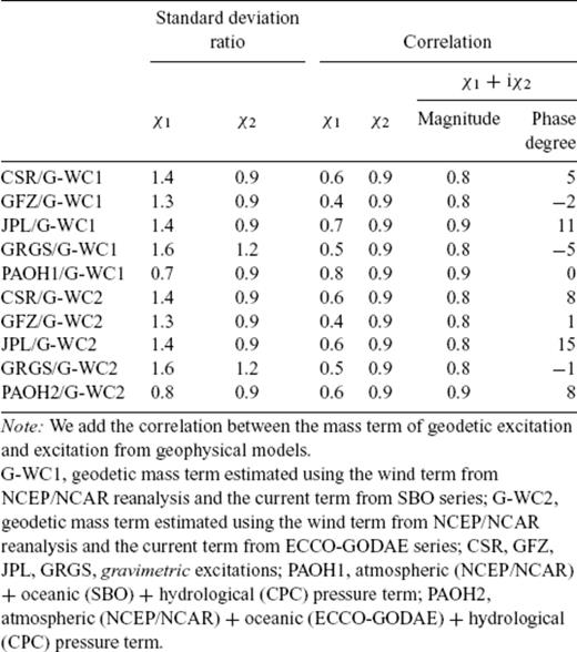
Correlation coefficients between the ‘gravimetric’ excitation and the mass term of the ‘geodetic’ excitation

Open in new tabDownload slide

That points out the defect of the modelling of the coupled oceanic-atmospheric influence on the oceans. Considering the excitation vector in the complex case, we find a similar level of correlation. There is, however, phase differences associated to all the series.

We also compare the standard deviation of the gravimetric based excitation with that one of the geodetic excitation (restricted to its mass term). As also shown in Table 2, there is globally more power in gravimetric based excitation (0–50 per cent more) for χ₁ component and less power in gravimetric based excitation for χ₂ component (10–20 per cent less). As for the correlation, the agreement in standard deviation is globally better for χ₂ component Differences between the centres solutions may be associated with the background models and satellite data processing for obtaining the spherical harmonics coefficients. However, we note that the agreement is globally better than those obtained for the previous release (Nastula et al. 2007).

Amplitudes and phases of the annual harmonic found in the gravity signal (Fig. 3) are consistent except for the GRGS solution, which has discordant phase value in the annual retrograde band. The semi-annual variations are three times smaller and not well determined by the least-square analysis.

Figure 3.

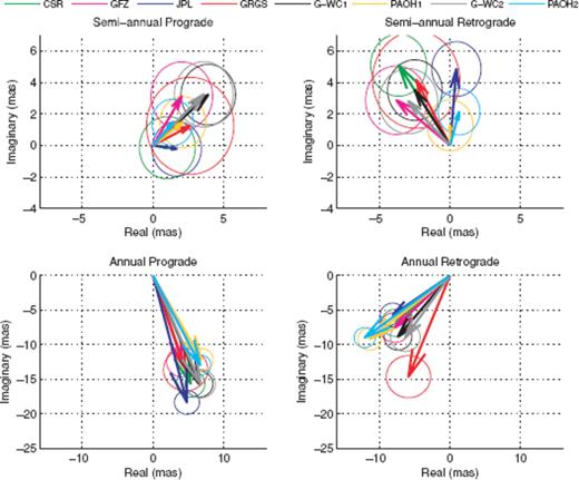
Phasor diagram of annual and semi-annual variations of the mass term of polar motion excitation computed from GRACE solutions, from ‘geodetic’ excitation and from geophysical fluids models. The circle radiuses represent the standard error of the least-square estimate. G-WC1, geodetic mass term estimated using the wind term from NCEP/NCAR reanalysis and the current term from SBO series; G-WC2, geodetic mass term estimated using the wind term from NCEP/NCAR reanalysis and the current term from ECCO-GODAE series; CSR, GFZ, JPL, GRGS, ‘gravimetric’ excitations; PAOH1, atmospheric (NCEP/NCAR) + oceanic (SBO) + hydrologic (CPC) pressure term; PAOH2, atmospheric (NCEP/NCAR) + oceanic (ECCO-GODAE) + hydrological (CPC) pressure term.

Open in new tabDownload slide

4 Comparison of the Residual Excitation

The main question is whether GRACE can contribute to a better estimate of the total mass term than the one associated with the combined atmospheric, oceanic and hydrological excitation. We will show later on that GRACE data are still very noisy.

The excitation residuals, after accounting for mass effects derived from the combinations of geophysical fluids, are smaller and smoother that those computed using GRACE GRACE releases 2 and 3 (RL02 and RL03, as Nastula et al. (2007) have shown. Here, we expand these analyses by using polar motion excitation functions computed from the RL04 release and from the GRGS solution.

Fig. 4 shows the different time-series of excitation residuals, computed using either the gravimetric data from CSR, GFZ, JPL and GRGS or the combinations of atmospheric, oceanic and hydrological series (PAOH). The two above-mentioned oceanic computation (ECCO_kf049f from SBO, ECCO—GODAE) are used for the oceanic contributions. The latter residuals are smoother than those computed from CSR, GFZ, JPL and GRGS data, which have more month to month variability, probably due to noise in the monthly estimates. This confirms results obtained by Nastula et al. (2007). According to Fig. 4, standard deviation of the gravimetric based residuals are larger (from 6 to 8 mas) than those based on geophysical model, in the case of the χ₁ component. This is much larger than the uncertainty of the geodetic excitation function (<1 mas). However, in the case of χ₂, residuals using gravimetric data and residuals based on the geophysical models have similar level of standard deviations, especially in the case of the GFZ and JPL based series. This is a very encouraging result since the noise in the monthly estimates seems to be reduced. Improvements in the future GRACE solutions could provide geophysical constraints to models or better understanding effects of mass redistributions on polar motion.

Figure 4.

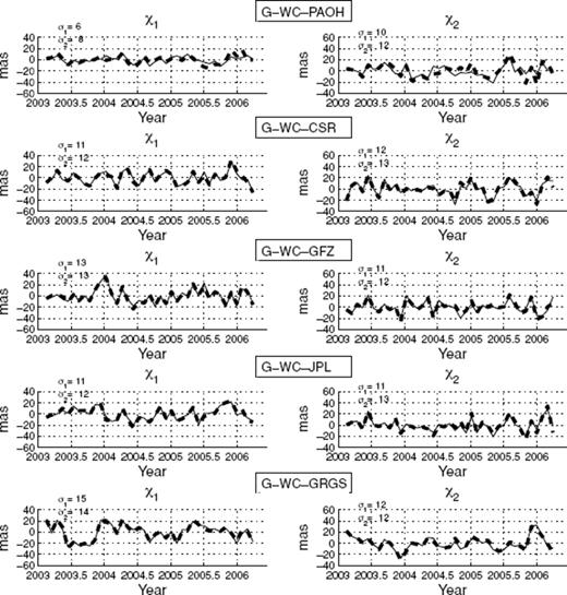
Residual equatorial excitation functions χ₁ (left-hand panel) and χ₂ (right-hand panel): ‘gravimetric’ excitation (CSR, GFZ, JPL, GRGS) or mass term of the excitation from geophysical fluids models (PAOH) have been removed from mass part of geodetic excitation (G-WC). In the geophysical models, we used CPC data for compute hydrological excitation and NCEP/NCAR reanalyses data for atmospheric excitation. For estimating oceanic effects two series are used: OAM series from SBO (continuous curves) and experimental series of ECCO-GODAE project (discontinuous curves). σ₁ and σ₂ are the standard deviation of series, the first, σ₁, for the series computed with ECCO from SBO and the second, σ₂, for the experimental series.

Open in new tabDownload slide

Correlation coefficients and standard deviation ratios between gravimetric based residuals and model based residuals are given in Table 3. They are significant differences in correlation when SBO oceanic excitation series or the ECCO—GODAE experimental series are used for removal ocean effects, especially affecting the χ₁ component, more sensitive to oceanic signals than χ₂. Using ECCO—GODAE estimates, the correlation with the CSR and JPL based residuals increases to 0.4. This shows some common features in the residuals stemming from the geophysical models. In the other case, residuals are not correlated (correlation value 0–0.1).

Table 3.

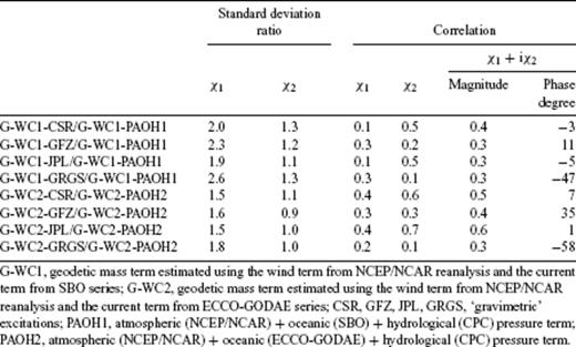
Correlation coefficients between the residual excitation obtained by removing from the mass term of geodetic excitation the ‘gravimetric’ data or the geophysical fluids models.

Open in new tabDownload slide

On the other hand, the gravimetric based residuals can be interpreted as a difference between the measured motion term (G-GRACE) and the modelled motion term. These residuals could be used to check the motion term models' (winds and currents) performance, whenever the mass term is well determined by GRACE observations.

5 Conclusions

Due to improvements in the background models, the CSR latest release is significantly better correlated to geodetic observations than the solution based on former GRACE releases 1, 2 and 3 (RL01, RL02 and RL03). We also confirm the agreement of GFZ and JPL series with the geodetic excitation found by Nastula et al. (2007). We show that the GRGS is also well correlated. However, largest correlation is still provided by the geophysical fluids models combination.

There are discrepancies between the various GRACE derived excitations (up to 20 mas) due to the different data processing applied for each centre. The residual signals are smoother when the modelled mass term is removed from geodetic excitation than those computed using gravimetric data. The latter residuals are larger in the case of χ₁. This component seems to be more sensitive to the background models errors. In the case of χ₂, the residuals are comparable, particularly for the JPL and GFZ solution. For this equatorial component, month to month variability, probably due to noise in GRACE solutions, is reduced. The improvements obtained in the last release are encouraging. Future releases of GRACE solution will probably lead to a better understanding of polar motion excitation and help to improve geophysical models.

We checked also the impact of the choice of the different OAM series. As expected, χ₁ is more affected than χ₂. For the residuals, significant differences in correlation values are found. Best correlation values are obtained from when ECCO—GODAE experimental series are used. It means that some common features exist. At this level, it is difficult to provide a reliable conclusion due to the high level of noise in the GRACE data.

Acknowledgments

We are grateful to Jean Michel Lemoine for providing us description of the GRGS solution, Rui Ponte for making available ECCO-GODAE experimental oceanic angular momentum series, David Salstein for his suggestions and Olivier de Viron for fruitful discussions. We thank the anonymous reviewers and Richard Gross for their helpful comments. Visit by Jolanta Nastula IERS to EOP PC Observatoire de Paris was sponsored by the Observatoire de Paris. Jolanta Nastula acknowledges the support of project N526 140 735 from the Polish Ministry of Science and Higher Education.

References

Appendix

Appendix: Acronyms

Open in new tabDownload slide