


Summary
The southern African Plateau is marked by anomalously high elevations, reaching 1–2 km above sea level, and there is much debate as to whether this topography is compensated by a lower mantle source or by elevated temperatures in the upper mantle. In this study, we use S-wave receiver functions (SRFs) to estimate the lithospheric thickness and sublithospheric mantle velocity structure beneath the Kaapvaal craton, which forms the core of the Plateau. To fit the SRF data, a low-velocity zone (LVZ) is required below a ∼160-km-thick lithospheric lid, but the LVZ is no thicker than ∼90 km. Although the lid thickness obtained is thinner than that reported in previous SRF studies, neither the lid thickness nor the shear velocity decrease (∼4.5%) associated with the LVZ is anomalous compared to other cratonic environments. Therefore, we conclude that elevated temperatures in the sublithospheric upper mantle contribute little support to the high elevations in this region of southern Africa.
Introduction
The depth extent of continental lithosphere beneath Archean and Proterozoic shields has been debated for many decades (e.g., MacDonald 1963; Jordan 1975), and much of this debate has revolved around the upper-mantle structure beneath the Kaapvaal craton in southern Africa (Fig. 1). Unlike many shields, which display average elevations 400–500 m above sea level, the surface topography in southern Africa reaches 1–2 km above sea level, with residual bathymetry in the surrounding oceans of more than 500 m (Nyblade & Robinson 1994). There is much controversy as to how this area of high topography, termed the ‘African Superswell’ (Nyblade & Robinson 1994), is compensated and whether it originates from either a lower- or upper-mantle source of buoyancy. Lithgow-Bertelloni & Silver (1998) and Gurnis et al. (2000), for example, suggested that dynamic topography generated by a large-scale upwelling originating at the core-mantle boundary supports the high elevations across southern Africa. Other studies have suggested that buoyancy from a thermal anomaly in either the lithosphere (Nyblade & Sleep 2003) or the asthenosphere (Burke et al. 2003; Li & Burke 2006; Burke & Gunnell 2008) might support the superswell.
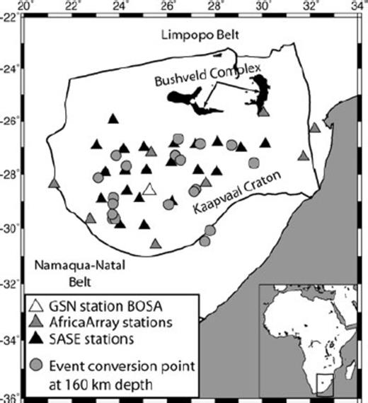
Stations from the SASE (black triangles) and AfricaArray (grey triangles) networks, along with GSN station BOSA (white triangle), used in this study. Grey circles show conversion points at 160 km depth from events meeting the SRF criteria. Bold lines outline the boundaries of labelled tectonic terranes.
To distinguish between these competing models, many studies have examined the upper-mantle velocity structure beneath parts of southern Africa. Evidence of a thermal anomaly in the uppermost mantle may be manifested either as an anomalously thin lithospheric lid with lower than average lid velocities or as an anomalously large or an anomalously slow low-velocity zone (LVZ). Results from modelling regional P waves, as well as body wave tomography, show high velocities extending to 300–400 km depth beneath southern Africa, with little evidence for a LVZ beneath the region (Zhao et al. 1999; James et al. 2001; Fouch et al. 2004). Inversion of fundamental mode surface-wave phase delays displays radial anisotropy throughout the upper mantle but no LVZ, indicating a thick lithosphere (Freybourger et al. 2001; Saltzer 2002). Inversion of both two-station fundamental-mode Rayleigh wave phase velocities and multiscale finite-frequency Rayleigh wave phase residuals yield similar results (Larson et al. 2006; Chevrot & Zhao 2007). However, other studies using multimode high-frequency surface wave data (Priestley 1999; Priestley et al. 2006) and Rayleigh wave tomography (Li & Burke 2006) find a high velocity lid beneath much of southern Africa, with a lid thickness between 160–200 km for the Kaapvaal craton, underlain by a ∼150 km thick LVZ associated with a ∼4% shear velocity (VS) decrease. Joint modelling of regional SH waves and mineral physics data also suggests a pronounced LVZ beneath southern Africa, with VS reductions of at least 5% beneath a 150-km-thick, high-velocity lithospheric lid (Wang et al. 2008). A 150–200-km-thick lid beneath the Kaapvaal craton is consistent with lithospheric thickness estimates inferred from heat flow measurements and from pressure-temperature estimates, based on kimberlite nodule data (Ballard & Pollack 1988; Jones 1988; Rudnick & Nyblade 1999; Artemieva & Mooney 2001; Deen et al. 2006; Priestley et al. 2006), but these data sets do not provide constraints on the nature of the LVZ.
In this study, we use the S-wave receiver function (SRF) technique (e.g., Farra & Vinnik 2000; Li et al. 2004; Kumar et al. 2007) to determine the depth to the lithosphere-asthenosphere boundary (LAB) by identifying S-to-P (Sp) conversions from discontinuities beneath seismic stations in the Kaapvaal craton. Unlike P-wave receiver functions (PRFs), where crustal multiples can mask conversions from the LAB, boundary conversions on SRFs can be more clearly identified because they arrive earlier than the direct S phase whereas all crustal multiples arrive later (e.g. Farra & Vinnik 2000; Li et al. 2004; Kumar et al. 2007). SRFs have been used in several previous studies to investigate the lithospheric structure beneath southern Africa (Kumar et al. 2007; Wittlinger & Farra 2007), but new methodological approaches and data selection criteria warrant a re-examination of those results. Our SRF analysis focuses on Sp conversions within the southern and central Kaapvaal craton to reassess both the lithospheric thickness and upper-mantle velocity structure beneath this region. This approach provides new insight into what role the LVZ, if one exists, plays in supporting the high elevation in this region of the African Superswell. Our results indicate a ∼160-km-thick lid beneath the craton, thinner than that interpreted in previous SRF studies (Kumar et al. 2007; Wittlinger & Farra 2007). Additionally, we demonstrate that a LVZ is required to fit the SRF data, but the VS decrease associated with the LVZ as well as the thickness of the lithospheric lid are not anomalous compared with other cratonic environments.
Data And Methodology
Teleseismic waveform data recorded at various Southern Africa Seismic Experiment (SASE; Carlson et al. 1996), AfricaArray (http://africaarray.psu.edu) and Global Seismographic Network (GSN) broad-band stations throughout the Kaapvaal craton were used in this study (Fig. 1). The SASE stations were deployed between 1997 April and 1999 July, and most of the AfricaArray stations were installed in early- to mid-2006; so, each of these networks provides about 1.5–2 yr of data. Significantly more data were recorded by GSN station BOSA, which has been operating since 1993 February. We selected S waves with high signal-to-noise ratios recorded at these stations from earthquakes with magnitudes larger than 5.7, depths less than 240 km and distances between 60° and 80°. It has been shown that this depth and distance criteria isolates true Sp phases from potential contamination by other P-wave phases (Wilson et al. 2006). Our event selection differs from that used in the Kaapvaal SRF study by Wittlinger & Farra (2007), who incorporated events with epicentral distances up to 110°.
Waveforms were first rotated from the N-E-Z to the R-T-Z coordinate system using the event's backazimuth and were visually inspected to pick the S-wave onset. The three-component records were then cut to focus on the section of the waveform that is 100 s prior to and 12 s after the S arrival. To detect Sp conversions, the data must be rotated around the incidence angle into the SH–SV–P coordinate system (Li et al. 2004). This second rotation is critical because if an incorrect incidence angle is used, noise can be significantly enhanced, and converted phases may become undetectable. The optimal incidence angle was determined using the approach of Sodoudi (2005), as described by Hansen et al. (2007). Using Ligorria & Ammon's (1999) iterative time domain method, SRFs are generated by deconvolving the SV component from the corresponding P component. To make the SRFs directly comparable with PRFs, both the time axes and the amplitudes of the SRFs were reversed (e.g. Farra & Vinnik 2000; Li et al. 2004; Kumar et al. 2007). The frequency content of the receiver function is controlled by the Gaussian width factor, a (Ligorria & Ammon 1999). Several values of a were examined; however, the best and most consistent results were obtained using an a of 1.0.
Once receiver functions were generated for all events at each station, the data set was subjected to a number of quality control criteria not employed in previous SRF studies (e.g. Kumar et al. 2007; Wittlinger & Farra 2007). Each receiver function was first compared with previously determined PRFs at the same station to identify the crust-mantle boundary (Moho) conversion. Across our study area, the crustal thickness is fairly uniform, ranging from about 36 to 41 km (Nguuri et al. 2001; Kgaswane et al. 2006, 2008). Only SRFs that display a clear Moho conversion at the appropriate time were used for further analysis. Next, the amplitude of the Moho conversion was examined. Forward modelling was used to predict the expected Moho amplitude using published averaged velocities for the crust and upper mantle (Niu & James 2002; Larson et al. 2006; Li & Burke 2006; Nair et al. 2006; Wang et al. 2008). If the amplitude of the Moho conversion on the SRF was significantly too large or too small (±3σ), indicating an unrealistic velocity contrast across the crust-mantle boundary, the SRF was discarded. Additionally, the conversion points of each SRF were examined to ensure the same tectonic terrain is sampled. For this study, we focused on the southern and central Kaapvaal craton to avoid potential bias from structural complexities associated with the Bushveld Complex in the northern part of the craton and the mobile belts surrounding the craton (Fig. 1). Previous studies indicate that the lid structure across the southern and central Kaapvaal craton is fairly uniform (Fouch et al. 2004; Li & Burke 2006). After high-grading the data set in this manner, we were left with several tens of records, representing about 10% of the original data set. The percentage of useable, high-quality data used in our SRF analysis is comparable to that typically used in PRF analysis for southern Africa (Kgaswane et al. 2006, 2008); however, fewer events overall are available for SRFs compared with PRFs, given the more restricted depth and distance range used.
To improve the signal-to-noise ratio and to convert to depth, individual SRFs were moveout corrected and stacked. In previous studies, moveout correction was applied using a specified reference slowness (6.4 s deg−1 in Kumar et al. 2007; 8.4 s deg−1 in Wittlinger & Farra 2007), and conversion to depth was performed using either a simplified local (Kumar et al. 2007) or global (Wittlinger & Farra 2007) velocity model. In our approach, individual, high quality SRFs were corrected and stacked using the method of Owens et al. (2000; Fig. 2). A variety of models with crustal and upper-mantle velocities appropriate for southern Africa (Niu & James 2002; Larson et al. 2006; Li & Burke 2006; Nair et al. 2006; Wang et al. 2008) were examined to optimize the stack and constrain discontinuity depths; however, the discontinuity depths varied by only ∼5 km depending on the choice of model. The final stack was produced using a modified version of the IASP91 model (Kennett & Engdahl 1991), with a faster upper crust of 3.5 km s−1, more appropriate for southern Africa (e.g. Nguuri et al. 2001; James et al. 2003; Kgaswane et al. 2006). 2σ bootstrap errors for the stack were determined using 200 randomly resampled sets of the data (Efron & Tibshirani 1991).
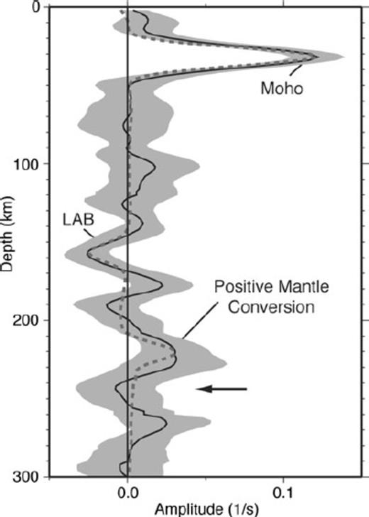
Stacked SRF showing the structure of the central and southern Kaapvaal craton. The solid black line shows the mean stack while the light grey shaded areas indicate the 2σ bootstrap error bounds. The grey dashed line shows an example of the synthetic SRF fit (from model B in Fig. 3). Major converted phases are labelled. The black arrow indicates the depth of the LAB reported by Kumar et al. (2007).
To further constrain the velocity structure, the SRF stack was modelled with synthetic receiver functions generated by the reflectivity method (Randall 1994). Using a limited grid search procedure, simple 1-D models were constructed for a range of lithospheric mantle VS values. The VS of the crust, LVZ, and sublithospheric mantle, as well as the boundary depths of the Moho and LAB, were then allowed to vary for each lid VS to match the amplitude and timing of conversions on the stacked SRF (Fig. 2). Crustal Poisson's ratio values were taken from Nair et al. (2006), whereas the Poisson's ratio at deeper depths was set to be the same as IASP91 (Kennett & Engdahl 1991). We did not attempt to model the sharpness of the discontinuities, but rather focused on determining the average layer thicknesses and velocity contrasts needed to fit the observed Sp conversions.
Results
The stacked SRF displays three Sp conversions with robust signals above the 2σ uncertainty level. The shallowest, positive conversion at ∼34 km depth (Fig. 2) is best interpreted as the Sp conversion from the Moho, and the amplitude of this conversion requires a ∼20% velocity increase across the crust-mantle boundary. These crustal estimates match well the results of previous studies across the central and southern Kaapvaal craton (Nguuri et al. 2001; Niu & James 2002; James et al. 2003; Kgaswane et al. 2006, 2008; Nair et al. 2006). The trough at ∼160 km depth marks the only substantial negative conversion on the stack (Fig. 2) and is best modelled as the LAB. To fit the amplitude of this trough, a velocity decrease of ∼4.5% is required. An additional, positive Sp conversion at ∼225 km depth is also observed, corresponding to a velocity increase of ∼3.5% (Fig. 2). This conversion may correspond to the Lehmann discontinuity (Lehmann 1961) and is comparable to the ‘220 discontinuity’ included in the global Preliminary Reference Earth Model (PREM; Dziewonski & Anderson 1981). Modelling of the 2σ bootstrap confidence limits was used to constrain the range of velocities and depths that fit the stacked SRF. On average, boundary depths are resolved to within about ±9 km, and the velocities are resolved to within ±0.11 km s−1 (Fig. 2).
Although receiver functions constrain velocity contrasts across discontinuities and vertical traveltimes, they do not uniquely constrain the subsurface velocity structure (Ammon et al. 1990). Therefore, to further test our SRF models, we compared the dispersion curves predicted by the models to observed dispersion measurements. Fig. 3 (inset) shows three different models, with fixed lid velocities ranging from 4.43 to 4.63 km s−1, which fit the mean stacked SRF. These models are constrained down to ∼225 km; velocities at deeper depths were set to match the modified IASP91 model used to convert the SRF to depth (Kennett & Engdahl 1991). Forward modelling was used to predict the Rayleigh wave phase velocities from each model, and these values were compared with dispersion data for the southern and central Kaapvaal craton from Li & Burke (2006). The predicted dispersion curves from these models bracket the dispersion data (Fig. 3), indicating that our SRF models are consistent with surface wave observations. If the models are allowed to vary within the SRF 2σ bootstrap error estimates, an even closer match to the dispersion data can be obtained (Fig. 4). SRF models with lid velocities faster than ∼4.6 km s−1 do not fit the phase velocity data.
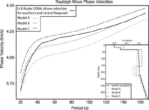
(inset) Three models (dashed lines) with different, fixed lid velocities that fit the mean stacked SRF (Fig. 2). These models are tied back to the modified version of IASP91 (solid black line) at depth. (main) Predicted Rayleigh wave phase velocity dispersion curves (dashed lines) from the three models in the inset compared to phase velocity data for the central and southern Kaapvaal Craton (Li & Burke 2006; black line).
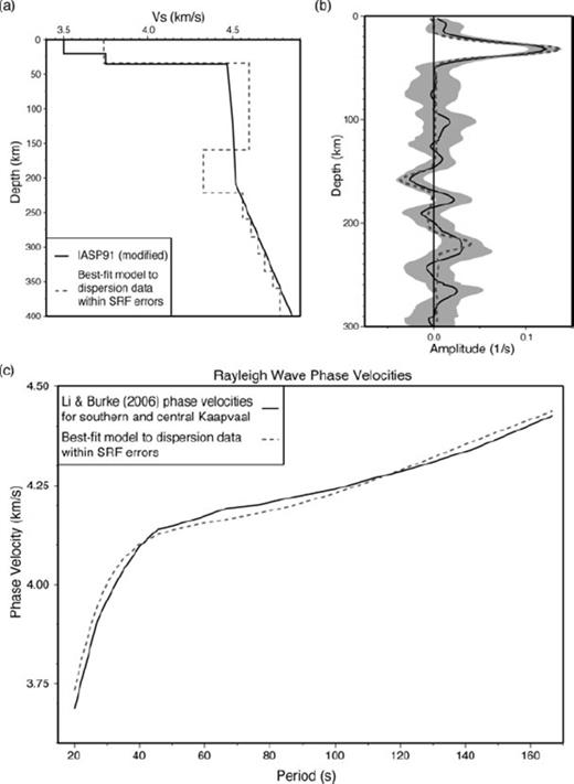
(a) Model providing the closest fit to both the stacked SRF and dispersion data, tied back to the modified IASP91 model at depth. (b) The solid black line shows the mean stacked SRF from Fig. 2. The grey dashed line shows the fit from the model in (a). Although this model does not fit the mean stack, it is still within the 2σ bootstrap error bounds. (c) Predicted Rayleigh wave phase-velocity dispersion curve (grey dashed line) from the model in (a). A close match to the phase velocity data for the central and southern Kaapvaal craton (Li & Burke 2006; black line) is obtained.
Discussion
Our SRF analysis was focused on determining the average layer thicknesses and velocity contrasts needed to fit the observed Sp conversions. The lithospheric thickness and LVZ velocity estimates obtained agree well with those from previous studies. Li & Burke (2006) imaged a fast mantle lid beneath the southern and central Kaapvaal craton to an average depth of 180 ± 20 km, underlain by a LVZ with a ∼4%VS decrease. Priestley (1999), Priestley et al. (2006) and Wang et al. (2008) required a LVZ with at least a 5%VS decrease beneath a 150–160-km-thick lithospheric lid to fit their observations; however, it should be noted that these models are for both Archean and Proterozoic terrains. Each of the above studies also indicates that the thickness of the LVZ is >150 km (Fig. 5). In contrast, the positive conversion on the stacked SRF at ∼225 km (Fig. 2) indicates a velocity increase, which may be due to chemical or compositional changes or to a transition from relaxed to unrelaxed moduli (Anderson 2007). Even with the associated error, this velocity increase implies that the LVZ is at most ∼90 km thick beneath the Kaapvaal craton. It should also be noted that these previous studies (Li & Burke 2006; Priestley 1999; Priestley et al. 2006) indicate faster lid velocities of about 4.70–4.75 km s−1 (Fig. 5), which cannot simultaneously satisfy the SRF and Rayleigh wave phase velocity data. The LVZs in these models extend down to ∼350 km depth, with velocities up to 4% slower than IASP91 below ∼250 km (Fig. 5). We believe that trade-offs between velocities in the lid and velocities in the sublithospheric mantle may explain the differences observed in the thickness of the LVZ.
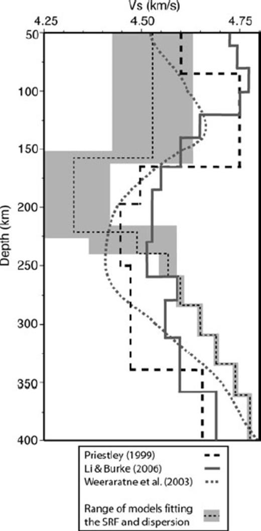
Comparison of the range of models fitting the stacked SRF and dispersion data (thin dashed black line with shaded grey limits) with shear velocity models for the Kaapvaal craton from Priestley (1999; bold dashed black line), Li & Burke (2006; solid grey line), and Weeraratne et al. (2003; dashed grey line), all of which display a LVZ in the upper mantle.
Our interpretations differ from those of previous SRF studies examining the Kaapvaal craton (Kumar et al. 2007; Wittlinger & Farra 2007). As mentioned previously, several differences in methodology and data selection criteria exist between those studies and our study, leading to variations in the SRFs obtained. For example, Kumar et al. (2007) interpreted two Sp conversions on their stacked SRFs: a shallow, positive conversion from the Moho and a deeper, negative conversion from the LAB. For GSN stations BOSA and LBTB, they reported LAB depths of 257 and 293 km, respectively, and the models presented to match the Sp traveltimes imply a ∼13% velocity decrease across the LAB. Unlike our approach, Kumar et al. (2007) corrected the SRFs for moveout using a reference slowness of 6.4 s deg−1 and determined boundary depths using a simple, three-layer velocity model with fixed VS in the crust, lithosphere and asthenosphere. Additionally, our study employs more rigorous quality control criteria. Our stacked SRF displays a trough at a similar depth as that interpreted by Kumar et al. (2007); however, this trough falls within the 2σ bootstrap errors (Fig. 2). The amplitude of this trough is also more subdued on our stack than that shown by Kumar et al. (2007), and no other study in southern Africa has imaged a LVZ with a 13%VS decrease beneath the Kaapvaal craton (Priestley 1999; Weeraratne et al. 2003; Li & Burke 2006; Priestley et al. 2006; Wang et al. 2008).
In another SRF study, Wittlinger & Farra (2007) examined multiple Sp conversions beneath the Kaapvaal craton. They interpreted a trough at ∼350 km on their stacked SRFs as the LAB whereas a shallower trough at ∼160 km (similar to that seen in our results) was interpreted as being the base of an anisotropic region in the upper mantle. However, their LAB interpreted trough is only resolved within a 1σ uncertainty level, and both isotropic and anisotropic velocity models predict comparable SRFs (Figs 4d-e in Wittlinger & Farra 2007). Similar to Kumar et al. (2007), Wittlinger & Farra (2007) corrected the SRFs for moveout using a reference slowness (8.4 s deg−1) and converted to depth using an assumed model (AK135; Kennett & Engdahl 1995). Additionally, Wittlinger & Farra (2007) incorporated events with epicentral distances up to 110° in their analysis, which may be contaminated by other teleseismic phases (Wilson et al. 2006) and mixed events whose Sp conversion points sample different tectonic terrains.
The average lid thickness and VS reduction in the LVZ beneath the Kaapvaal craton, inferred from both the SRF analysis and from previous studies (e.g. Priestley 1999; Li & Burke 2006; Priestley et al. 2006; Wang et al. 2008), are ∼160 km and ∼4.5%, respectively, which are comparable to other cratonic environments. Kustowski et al. (2008a,b) investigated the upper-mantle structure beneath the Eurasian and other cratons using a tomographic model developed from surface-wave phase velocities, body wave traveltimes, and long-period waveforms. They found fast-velocity anomalies at 150 km depth beneath the East European Platform, Siberia, and Tibet, but that these fast velocities nearly vanish by 250 km. A similar, strong velocity decrease between 150 and 250 km is also observed beneath other cratons in North America, South America, and Australia, and Kustowski et al. (2008a,b) suggest that this dramatic velocity decrease likely represents the base of stable continental lithosphere.
Weeraratne et al. (2003) compared the velocity structure beneath various Archean cratons using global data sets of fundamental mode Rayleigh wave phase velocities. Eight cratons were examined, including the Kaapvaal, Tanzanian, Canadian, Siberian, Indian, SinoKorean, Yilgarn, and Amazonian cratons. In all cases, LVZs were observed at depths ranging from 150–250 km. With the exception of the Tanzanian craton, where the VS reduction associated with the LVZ was ∼10%, the LVZ beneath all other cratons was found to be associated with a VS reduction of ≤ ∼6% (Fig. 5; Weeraratne et al. 2003). Grand & Helmberger (1984) examined the velocity structure beneath the Canadian Shield and inferred a ∼150-km-thick, high-velocity lithospheric lid overlying a LVZ, associated with a ∼4%VS decrease. Similar observations have also been made beneath western Australia (Simons et al. 1999) and the Baltic Shield (Olsson et al. 2007).
Conclusions
Given that the LVZ beneath the Kaapvaal craton is not anomalously slow and that the lithospheric lid of the craton is not anomalously thin, we conclude that elevated temperatures in the sublithospheric upper mantle do not contribute substantially to the support of high surface elevations in this region of the African Superswell. Cratons elsewhere are characterized by similar lid thicknesses and are underlain by similar LVZs, but they do not display unusually high surface topography like that observed in southern Africa. Therefore, other compensation mechanisms for this portion of the Superswell are likely. For example, excess heat in the lithosphere, resulting from multiple plume events, could have generated uplift in southern Africa without leaving a detectable seismic signature. By combining the effects of ponded plume head material at the base of the lithosphere, with additional buoyancy from plume tails lingering beneath the lithosphere for 25–30 Myr, it is possible to account for the present-day elevation of southern Africa (Nyblade & Sleep 2003). Alternatively, a large-scale upwelling originating at the core-mantle boundary may compensate the Superswell topography. Lower-mantle density perturbations are necessary to reproduce the pattern and amplitude of dynamic topography in southern Africa (Lithgow-Bertelloni & Silver 1998; Simmons et al. 2007), and a large upwelling is consistent with mantle flow models and seismic anisotropy studies (Gurnis et al. 2000; Panning & Romanowicz 2004).
Acknowledgments
We thank Randy Keller, Mark Muller and an anonymous reviewer for their thorough critiques of this manuscript. Support for this work has been provided by the National Science Foundation, grant 0530062. Figures were prepared using GMT (Wessel & Smith 1998).
References
