


Summary
We use correlations of the ambient seismic noise to study the crust in western Europe. Cross correlation of 1 year of noise recorded at 150 three components broadband stations yields more than 3 000 Rayleigh wave group velocity measurements. These measurements are used to construct Rayleigh group velocity maps of the Alpine region and surrounding area in the 5–80 s period band. In the 5–10 s period band, the seismic noise recorded in Europe is dominated by surface waves originating from the Northern Atlantic ocean. This anisotropy of the noise and the uneven station distribution affect the azimuthal distribution of the paths where we obtain reliable group velocity measurements. As a consequence our group velocity models have better resolution in the northeast direction than in the southwest direction. Finally we invert the resulting Rayleigh wave group velocity maps to determine the Moho depth. Our results are in good agreement with the result of the numerous active experiments in the Alps and provide a continuous image of the Alpine structure.
1 Introduction
Accurate high-resolution imaging of the crust is necessary to understand the interaction between mantle dynamics and near surface geological processes. Observational methods in seismology are typically based on earthquake seismograms or rely on active sources. Specifically, surface wave tomography has traditionally exploited the frequency-dependent wave velocity (dispersive) characteristic of Love and Rayleigh waves. Dispersion has been measured as an average property of the propagation path of earthquake waves traveling from an earthquake source to a station (e.g. Ekstrom et al. 1997; Ritzwoller & Levshin 1998) or between two stations with approximately the same azimuth or back azimuth with respect to the earthquake source (McEvilly 1964; Dziewonski & Hales 1972; Meier et al. 2004). When considering surface wave dispersion measurements along earthquake source-station paths, the resolution is limited by two main factors: (1) non-uniformity in the geographical distribution of earthquake sources and receivers, and (2) inherent attenuation and scattering of the high-frequency content of teleseismic records. The heterogeneous distribution of sampled Fresnel zones resulting from heterogeneous data coverage limits resolution in regions sampled by few or no raypaths. At teleseismic distances, most of the high-frequency information (≤20 s) is lost due to the attenuation and scattering of the medium. Surface waves sample the average material properties to a given depth and higher frequency signals sample shallower structure. Therefore, losing the high-frequency component of the earthquake signal limits the ability to image the crustal structure.
Recent theoretical and laboratory studies have demonstrated that the time cross correlation function of random wavefields computed at two distant receivers contains the Green's Function between these two receivers, that is the waveform that would be recorded at one of the stations if a point source is applied at the other station. (Weaver & Lobkis 2001; Lobkis & Weaver 2001; Colin de Verdière 2006a,b; Sánchez-Sesma et al. 2006a,b; Larose et al. 2006; Campillo 2006).
In seismology this idea has been successfully applied to the seismic coda (Campillo & Paul 2003; Paul et al. 2005) and seismic noise (Shapiro & Campillo 2004; Shapiro et al. 2005; Sabra et al. 2005a). Ideally, this gives us the possibility of measuring surface wave dispersion curves between any pair of stations of an array using only ambient noise records. Stehly et al. (2006) have shown that the seismic noise sources in the [5–20 s] period band are distributed over a large surface when integrated over a long time. Therefore, the randomness of the ambient seismic field is ensured mainly by the random spatial distribution of the sources when considering long time-series. Additional randomization is produced by seismic scattering on small-scale inhomogeneities within the Earth. Following the cross-correlation procedure of (Shapiro & Campillo 2004), we retrieve the Green's function between two stations by correlating background seismic noise records. The emerging signal is dominated by surface waves since the background seismic noise consists mainly of surface waves (e.g. Friedrich et al. 1998; Ekström 2001), and because the Green's function between two points at the free surface of the Earth is dominated by surface waves. The reconstructed Green's functions are stable over time and robust enough to measure group velocity dispersion to a few tenths of a second, independently of the azimuth of the considered station-station path (Stehly et al. 2007). Passive imaging from seismic noise has first been used to compute Rayleigh wave group velocity maps by Shapiro et al. (2005) and Sabra et al. (2005a).
More recently, noise based surface-wave tomography has been applied in Tibet (Yao et al. 2006), New Zealand (Lin et al. 2007), Korea (Kang & Shin 2006), Finland (Pedersen et al. 2007), and to produce large-scale Rayleigh wave group velocity maps across Europe (Yang et al. 2007). At a smaller scale, Brenguier et al. (2007) investigated the 3-D S-wave structure of the Piton de la Fournaise volcano. In this paper we apply seismic ambient noise correlation to study the lithosphere in western Europe. We use 150 broadband stations to determine the distribution of surface wave group velocities across the Alpine region and surrounding area in the 5–80 s period band. We then invert the resulting Rayleigh wave group velocity maps for a 3-D crustal structure and, in particular, to determine the Moho depth.
2 Data Processing
We used 1 year of continuous records from October 2004 to October 2005 at 150 three components broadband European stations. In the 5–10 s period band, the distribution of noise sources does not change with time, and using more than one month of data does not improve the Greens function reconstruction (Stehly et al. 2007). Above 10 s, the origin of the noise changes with the season but tends to be the same from year to year (Rhie & Romanowicz 2004; Stehly et al. 2006). For this reason, using more than 1 year of data does not improve significantly the traveltime measurements performed on noise correlations at least in the 5–50 s period band.
The data were obtained from the ETH Zürich, the Virtual European Broad-Band Seismic Network (VEBSN, http://www.orfeuseu.org/Data-info/vebsn.html), the IRIS database, the Commissariat à l'énergie Atomique (CEA, France), the Laboratoire de Géophysique internet et de Tectonophysiue (LGIT, France) and the RETREAT experiment. Our aim is to focus on the Alps, where the station density is particularly large (Fig. 1). All records were processed day per day. First, the 24-hr records were decimated to 1 Hz and were deconvolved from the instrument responses to ground velocity. Then the spectra of the records were whitened: we divided the amplitude of the noise spectrum by it absolute value between 5 and 150 s without changing the phase. The spectral whitening has two aims: first it corrects the spectrum of the noise that is dominated two peaks at 7 s and 14 s. Second it imposes that noise records for each day have the same energy between 5 and 150 s. This prevents the records to be dominated by energetic events such as stroms or earthquakes.

(a) Map showing the location of broadband recorders used for this study. (b) Schematic map of the boudaries between the Ligurian, European and Adriatic plate (red dots). The broadband stations used for this study are shown with blue triangles.
For each station pair, North and East horizontal components were rotated in the direction of the interstation azimuth to provide radial (R) and transverse (T) components of energy propagating directly along the great circle connecting the two stations. We then correlated signals recorded on the components that correspond to the surface wave term of the Green's function day by day.
As Rayleigh waves are polarized in the Z-R plane, the vertical and radial components were correlated in all four possible combinations (ZZ corresponding to a cross-correlation of the noise recorded at the two stations in the vertical direction, RR corresponding to both radial components, and both RZ and ZR corresponding to one radial and one vertical component each) to retrieve the Rayleigh wave Green's function. The correlation of both transverse components (TT) yields the Love wave Green's function. Correlations of 1-day records are then stacked. This is equivalent to directly cross-correlating the whole year of records. Note that compared to other studies (Shapiro & Campillo 2004; Sabra et al. 2005b; Shapiro et al. 2005; Yao et al. 2006; Yang et al. 2007), we did not apply any amplitude normalization, instead we whitened the spectrum of the records day per day.
2.1 Example of AIGLE-STU
Fig. 2 shows the ZZ cross correlation of 1 year of records between the stations AIGLE and STU, bandpassed into several period bands from 10 to 60 s. The interstation distance is 320 km. The positive time of the correlation corresponds to the causal Green's function of the medium between AIGLE and STU, and the negative time corresponds to its anticausal counterpart (i.e. the Green's function between STU and AIGLE). A wave train corresponding to Rayleigh waves is clearly visible on all period bands in the positive and negative correlation time at 100 s. This corresponds to a velocity of 3.2 km s−1. Dispersion is clearly seen with high-frequency waves arriving after low-frequency ones.
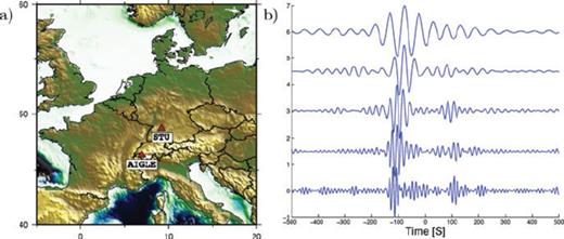
(a) Map of Europe showing the location of the two broadband stations AIGLE and STU (red triangle). (b) Cross-correlation of one year of records between AIGLE STU bandpassed in several period bands from 10 to 60 s.
In practice, correlations are generally not perfectly symmetric. In this example, the amplitude of the Rayleigh waves is larger for negative than for the positive time, although the phase arrival times are equal. This indicates that during the year 2004–2005 more energy propagated from STU to AIGLE than from AIGLE to STU. As most of stations record three component signals, we were able to retrieve Rayleigh waves by correlating the vertical and radial components (ZZ, RR, ZR, and RZ). Fig. 3(a) shows the correlations corresponding to Rayleigh waves for the AIGLE-STU path bandpassed in the 10–20 s period band. The arrival times are the same for all traces and the expected phase shift due to the elliptical polarization of Rayleigh waves between the ZZ and RZ correlations is visible. Similarly, Love waves are clearly visible on TT correlations. In the case of Fig. 3b), the Love wave appears only for negative correlation times. This asymmetry is a common feature within the set of paths analyzed here. It indicates that the noise source for Love waves is more localized than for Rayleigh waves (which exhibit two-sided correlation function in a much larger proportion). Note that, although the Love wave contribution to ambient noise is clearly attested by the correlation, its physical origin is still unclear. In absence of the redundant measurements which are possible for each path with Rayleigh waves, we expect less reliable evaluations of Love velocities. Actually since we were unable to perform joint Love and Rayleigh inversion, we decided to discard the Love speed measurements in the following.
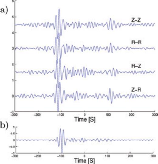
Cross-correlation of 1 year of records between AIGLE and STU bandpassed in the 10–20 s period band (a) Rayleigh waves obtained from ZZ, RZ, ZR and RR correlations and (b) Loves waves obtained from TT correlation.
3 Two-Dimensional Inversion
3.1 Selection of the paths
Rayleigh waves dispersion curves are evaluated from the emerging Green's functions using the frequency-time analysis (Herrmann 1973; Bhattacharya 1983; Ritzwoller & Levshin 1998; Levshin et al. 1989) for the 12 000 interstation paths. For every path, we measure eight possible Rayleigh wave dispersion curves by considering four components of the correlation tensor (ZZ, RR, RZ and ZR) and both the positive and the negative part of the noise correlation function.
To be selected in our dispersion analysis, correlations must meet several criteria. We define signal to noise ratio as the ratio of the amplitude of the Rayleigh wave and the standard deviation of the noise following Rayleigh waves. More precisely, the standard deviation of the noise is evaluated in a time window that starts at arrival time corresponding to a velocity of 1 km s−1, and finish at 4 000 s (i.e. if the interstation distance is 300 km, the standard deviation of the noise is evaluated in the positive correlation time from 300 to 4 000 s and in the negative correlation time from −4 000 s to −300 s). The signal-to-noise ratio is measured separately on the positive and negative correlation time at the discrete period at which we compute a group velocity map (5 s, 8 s, 12 s, …, 80 s).
Using noise crosscorrelations leads to redondant measurements and allows quality tests. We carefully selected high-quality measures. First at each period of interest, we reject waveforms with a signal-to-noise ratio ≤7. Then for each path, we have four correlations corresponding to Rayleigh waves (Z-Z, Z-R, R-Z and R-R) that leads to 8 measurements of the Rayleigh wave group velocity since we consider both the positive and negative correlation time. We keep only the correlations if the Rayleigh waves group velocities measured on the positive and negative correlation time differs by less than <5%. The retained measurements are then averaged for every path to get the final velocity.
We further reject records with interstation distances smaller than two wavelengths to prevent Rayleigh waves reconstructed on the positive and negative correlation time to overlap.
At 5 s, using these criteria result in selecting 3 400 Rayleigh wave observations from the initial 12 000 station pairs (Fig. 4). We achieve a path density that reaches 150 paths per 25 × 25 km cell in Switzerland (Fig. 4b). We obtain similar path densities at period up to 50 s. Above 50 s, the number of paths tends to decrease, and we choose to use a grid of 50 × 50 km instead. At 60 s, we selected 1 810 paths resulting in a density of more than 100 paths per cells in Switzerland.
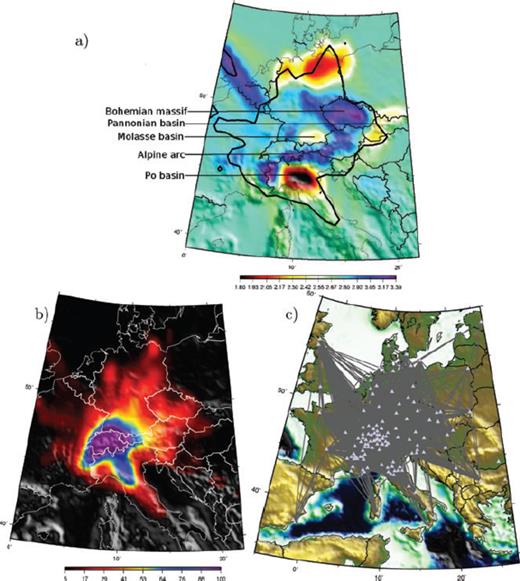
(a) Group velocity map for Rayleigh wave at 5 s period. The black line delimits the area where at least 10 paths are crossing each cell. (b) Map showing the number of paths crossing each cell for the 5 s Rayleigh paths. (c) 3400 paths where reliable group velocity measurement were obtained for 5 s Rayleigh waves.
3.2 Inversion method

Three regularization parameters are chosen prior to the inversion: α and β determine the weight that is given to the spatial smoothing and to the dependence of the perturbation magnitude with the path density. The correlation length σ controls the width of the spatial smoothing kernel. Because of the dense path coverage, we found that the results are not sensitive to the choice of β and λ in the region of highest density (central and western Alps and southern Germany). The correlation length was set to 25 km at periods between 5 and 40 s and 50 km for periods above 50 s. The value of α was chosen through a standard trade-off (L-curve) analysis by plotting the misfit as a function of α. Our preferred value of α lies near the maximum curvature of the L-curve.
3.3 Rayleigh waves group velocity maps
Group velocity maps are computed in two steps. (1) A first overdamped model including all selected paths is computed. The difference of the measured traveltime and the traveltime predicted by the inverted model is computed for every path. We discard all paths for which this time difference exceeds twice the time difference averaged for all paths. This concerns less than 3% of the selected paths. The rejected paths are mostly long paths (≥1 000 km) located outside our main region of interest (i.e. the Alps). (2) We compute the final group velocities map on a 25×25 km grid across Europe. The initial model used for the inversion has an homogeneous velocity equal to the average measured velocity.
Fig. 4 shows the obtained group velocity maps for 5 s Rayleigh waves. At this period, Rayleigh waves are mostly sensitive to shear velocities in the upper crust (3–7 km). Velocity anomalies correlate well with geological units. Low velocity regions are shown in red and black and correspond to sedimentary basins. The Po basin is clearly visible as well as are the North Sea basin and the Molasse basin. High-velocity areas shown in blue and purple correspond to the crystalline crust of the Alps and Bohemian Massif. Computed group velocities map for Rayleigh waves at 8, 16, 35 and 50 s are shown in Fig. 5. To compute these maps, we used a starting model with an homogeneous velocity of 2.8, 2.85, 3.35 and 3.75 km s−1, respectively.
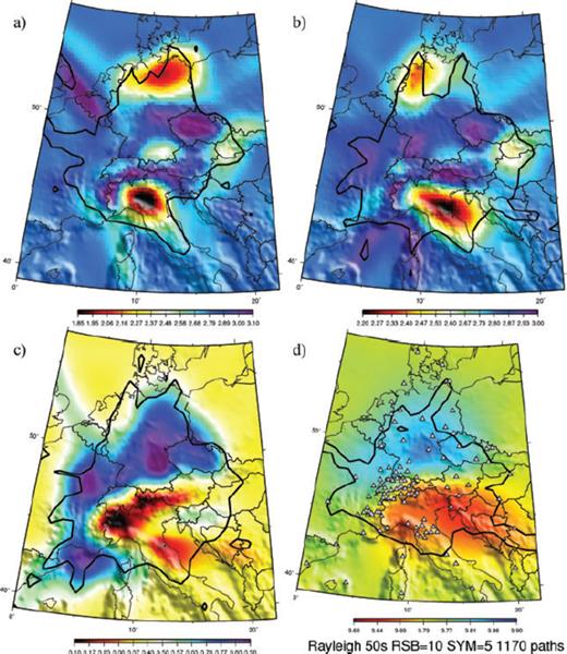
Rayeigh (left) waves group velocity maps at (a) 8 s (b) 16 s (c) 35 s. (d) 50 s.
8 s second surface waves are mostly sensitive to the upper crust (5–8 km). The Alpine arc and Bohemian Massif are associated with high velocities that can reach 3.2 km s−1. At 16 s, surface waves are sensitive to the middle crust. The main structures from the 8 s map are still present, but in addition the French and Swiss Jura is visible with high velocities reaching 3.0 km s−1. 35 s waves are mostly sensitive to the crustal thickness: in regions where the crust is thin, surface waves sample mantle higher velocities, whereas in regions where the crust is thick, they are associated with slower crustal velocities. The 35 s group velocity map shows a great contrast between area of average crustal thickness (Germany, central France, with high velocities), and areas where the crust is particularly thick (e.g. the Alps with low velocity, suggesting a thick crustal root).
3.4 Resolution of group velocity maps
The resolution of the group velocities maps depends mostly on the density of paths and on their azimuthal distribution. In our case, these two parameters depend on the geometry of the network and on the distribution of the noise sources that can limit the number of available paths for some directions. Resolution matrices are computed during the inversion as described by (Barmin et al. 2001). Each row of the resolution matrix is a map representing the resolution for one cell of the model. It quantifies how the obtained group velocity at one node depends on the measurements performed at others nodes. We define the resolution length at each node of the model as the distance for which the value in the matrix resolution has decreased by a factor 2. If the azimuthal distribution of paths is homogeneous, the resolution length is not expected to depend on the azimuth: the measurements obtained at one node depend on the measurements performed at adjacent nodes, with no preferential direction. However, because of the heterogeneous distribution of the stations and especially because of the uneven distribution of the noise sources in the 5–10 s period band the distribution of paths is not homogeneous: we have more paths oriented in the southeast direction than in others directions. As a consequence, the shape of our resolution surface is roughly elliptical: the resolution is better in the northeast direction than in the southeast direction (Fig. 7).
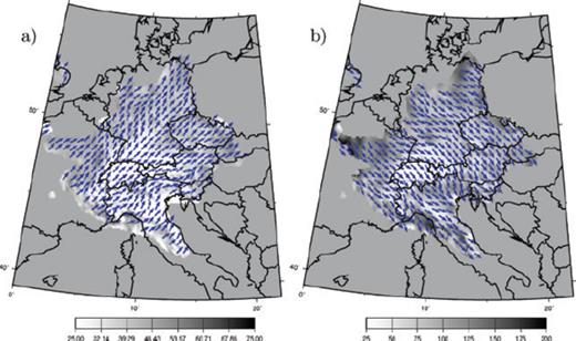
(a) Azimuth for which the resolution length of the 5 s Rayleigh group velocity map is the shortest. The color scale indicates the value of the resolution length for this direction. (b) idem for the direction where the resolution length is the larger.
At each node of the model, we measure the resolution length in direction corresponding to the direction of maximum and minimum resolution length. By averaging these two values we define the average value of the resolution length. Fig. 6(a) shows the average resolution length for the 5 s Rayleigh group velocity map in the area where we have at least 5 paths per cell. Maximum resolution is in Switzerland where the path density is the highest. In this area, we have a resolution length of 25–30 km. Peripheral to the central Alps (Southern Germany, eastern Austria, south-east France), the average resolution varies between 40 and 65 km. Outside this area the resolution is about 70 to 90 km.
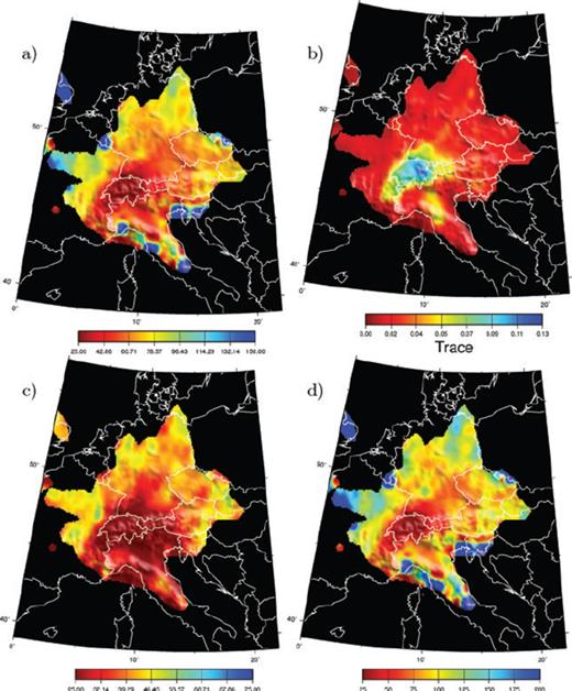
Resolution of the 5 s Rayleigh wave group velocity map. (a) Resolution length averaged in all directions (b) Trace of the resolution matrix (c) Value of the resolution length in the best direction (d) Value of the resolution length in the worst direction.
In the 5–10 s period band, we found that the resolution length is not isotropic. This is not observed at longer periods. Figs 7(a) and (b) show respectively the directions of maximum and minimum resolution length, and the average value of the resolution length. Two main factors explain that the resolution length depends on the azimuth in the 5–10 s period band: (1) the noise recorded in Europe is dominated by noise coming from the northern Atlantic ocean. The quality of the Green functions reconstruction is better for path oriented towards the Northern Atlantic Ocean, than in the perpendicular direction and (2) the convergence of the correlation towards the Green function is easier for short paths than for long paths.
As a result, in Germany where the interstation distance is large, we have more reliable group velocities measurements for path oriented towards the Northern Atlantic Ocean than in other directions. The resolution is about twice better in the northeast direction (40–45 km) than in the southeast direction (75–125 km). In Switzerland we have a higher path density and the interstation distance is much lower than in other areas. In this context, the convergence of the correlation towards the Green function depends less on the azimuth, and the resolution length is almost isotropic (i.e. we have the same value in the best and worst direction). This observation was made for the period band 5–10 s.
4 3-D Inversion
4.1 Method
Group velocity maps provide information about laterally varying surface wave velocities with respect to the period. From each cell of the model we extract the period-dependent velocities of Rayleigh waves from all the computed group velocity maps (5 s, 8 s, 12 s, 16 s, 18 s, 20 s, 25 s, 30 s, 35 s, 40 s, 50 s, 60 s, 70 s, 80 s), obtaining one dispersion curve for each cell.
Dispersion curves reconstructed for every cell are then inverted to obtain corresponding 1-D VS profiles. We use a simple four-layer parametrization: sedimentary layer, upper crust, lower crust and mantle. We use a non-linear Monte Carlo inversion with two iterations (Shapiro et al. 1997). In the first step of the inversion, we conduct a random search over much of the model space. We allow large variations of both the S velocity and the depth of each interface, and we tolerate large misfit values. The initial model is chosen with a Moho depth of 30 km, and a lower crustal limit at 15 km. Since our shortest period observations are at 5 s, we cannot constrain the thickness of the sedimentary upper crust. We use the sedimentary thickness provided by Crust2.0 (http://mahi.ucsd.edu/Gabi/rem.html) for the initial model. We allow for the thickness of the sedimentary layer to vary up to 1 km during the inversion. In the second step, we use the model with the lowest misfit from the first step as the ‘new’ initial model. Because we emphasize locating the crust-mantle boundary, we allow the VS to vary by 0.1 km s−1 in each layer, but we allow for large changes in layer thickness. We restrict the Moho depth to be between 20 and 60 km, and the sedimentary layer to less than 5 km thickness. As the solution of the inversion is non unique, we keep 10 best models.
4.2 Example of 1-D VS Profiles
Fig. 8 shows three examples of S-wave velocity profiles obtained at three cells of our model corresponding to diverse geological settings, the Po plain, the Austrian Alps, and the southern Germany. For each example, we show group velocity in the right panel with black dots and the dispersion curve associated with the 10 best VS profiles in solid lines on the left panel. For all the examples, we were able to model VS profiles which fit the measured dispersion curves. Although the inversions provide non-unique solutions, the depth of Moho in the series of chosen models varies only slightly. In Southern Germany, we found a Moho depth of about 30 km, that corresponds to a standard crust. In the Austrian Alps, the thickening of the crust is clearly visible, with a Moho depth of 45 km. In the Po Plain, all selected inverted models show a similar sedimentary layer at 2.5 km, and a Moho depth of 33 km.
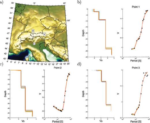
(a) Map showing the location where we present S-wave profile obtained after inverting Rayleigh wave dispersion curves. (b)–(d) Inversion of Rayleigh wave dispersion curve into S-wave velocity profile at 3 cells in the Po Plain, the Austrian Alps, and the Southern Germany. The right panel shows the measured Rayleigh waves dispersion curves (black dots) and the dispersion curves associated with 10 best Vs Profiles shown with solid lines on the left panel.
4.3 Map of Moho depth
Figs 9(a) and 10(a) show the inverted depths of the Moho. Whereas the inversion of group velocities was performed independently at each grid cell, the resulting distribution of crustal thickness is spatially consistent. The Moho depth varies between 25 and 55 km and two main areas can be distinguished: the European plate and the Adriatic plate. The boundary separating the two provinces corresponds to the southern terminus of the Alpine crustal thickening. A third unit, the Ligurian plate, is located at the southernmost part of the studied region (see Fig. 1). The main features of the Moho topography are explained by the interaction between these 3 units. The European lower crust is subducting southward under the shallower north-dipping Adriatic plate. At the same time, the Adriatic lower crust is subducting southward beneath the Ligurian plate. The Adriatic plate is compressed between the European plate in the North and the Ligurian plate in the South. In this area, beneath the northern Po Plain, we found the Moho at about 30 km. The central and western Bohemian Massif is characterized by a Moho at around 28 km. The transition from the average Moho of the Bohemian Massif and the thick crust of the Alpine region is very sharp and outlines the geometry of Alpine subduction. We find the Moho depth varying between 30 and 55 km within the Alps with maximum crustal thickness in southeastern Switzerland and east of the France-Italian border close to the Ivrea Zone.
![Results of the inversion of Rayleigh wave group velocity maps: a) Map of the Moho depth [km] b) Misfit of the Inversion [km s−1].](https://oup.silverchair-cdn.com/oup/backfile/Content_public/Journal/gji/178/1/10.1111/j.1365-246X.2009.04132.x/3/m_178-1-338-fig009.jpeg?Expires=1749871647&Signature=FHyIUtbiLynrcxe7-fdIOgTAyQsfxpWg1JEKqAifoS0iwfuPV4Bn8yatYeseANp5JaDo34wHs9wexswFslgm0C1WxHN5mhRC4w8wrYQU6gJ-BcttE5vsOJkNwL2LNvfyVK3mbhjdkMgu6qjhkgRsrigLujlkU2IqhQVU6GeF5sPDYvKk2vA6Tc5lGYxD5fPoUPDz3-meLleG7vmMIK9ddVeOTqLgi~gLhr24VSflNsGbqfPGN2GCosyaosp1nSj2fOR4UnU0AuA6nzFZiHuMkf~zOTh20ZHYE-92xJz~jqsk0zXGzqtkKWUjtbzZwG1GQ0Dw2ZE0LzpBN0dbVCvCHQ__&Key-Pair-Id=APKAIE5G5CRDK6RD3PGA)
Results of the inversion of Rayleigh wave group velocity maps: a) Map of the Moho depth [km] b) Misfit of the Inversion [km s−1].
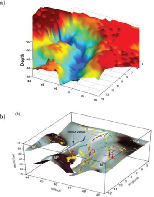
3-D view of the Moho depth a) from our results b) From Waldhauser et al. (1998).
The misfit of the inversion is shown in Fig. 9(b). Misfit of the model and measured data (<0.7 km s−1) within the central and western Alps is remarkably low. The model is characterized by higher misfit north of the Alps where the path density is smaller.
4.4 Comparison with other studies
The Alpine region has been studied intensively using controlled source and earthquake tomography. These studies provide insight into the crustal and upper mantle velocity structure (e.g. Marchant & Stampfli 1996; Waldhauser et al. 1998; Paul et al. 2001; Waldhauser et al. 2002; Marone et al. 2003; Bleibinhaus & Gebrande 2005; Thouvenot et al. 2007). Dèzes & Ziegler (2001) presented a Moho map of Europe resulting from the compilation of several seismological and gravimetric studies. The overall shape of their Moho map matches our results at locations where we have a high density of data coverage (southern Germany, Switzerland and Austria). Our Moho model within the alpine orogenic root is strikingly similar to the one obtained by Waldhauser et al. (1998). That study relied on published seismic reflection and refraction data of about 250 profiles across the Alpine region. They determined the simplest geometrical configuration of the Moho consistent with this data set. Their Moho map within the Alpine arc shows an overall good agreement with our result (Fig. 10). Although our results shares the same main characteristics there are one noticeable difference: Waldhauser et al. (1998) shows a fluctuation within the Adriatic plate at the southern most part of their model (around 44°N, 7°E), that is not visible in our model. However we believe that this difference is mostly due to our poor path coverage in this area.
5 Conclusion
We used 1 year of ambient noise records at 150 three components broadband European stations. Rayleigh wave Green's functions were retrieved by correlating the noise records between all station pairs. We selected the best waveforms using a criteria based on signal to noise ratio and time symmetry. About 3 500 reliable Rayleigh waves group velocities measurements at period below 50 s, and about 1 500 measurements at period above 50 s met these criteria. We used these measurements to perform Rayleigh wave tomography at periods ranging from 5 to 80 s using a 25 × 25 km grid below 50 s. The resulting group velocities maps feature numerous velocity anomalies that are correlative with known geological units.
At each cell of our model, we extracted Rayleigh waves dispersion curves from our group velocities map, and invert them using a two step Monte Carlo algorithm to determine the depth of the Moho in the Western Alps (Switzerland, Austria, southern Germany). Our results clearly show thickening of the crust below the Alps. Our map of Moho depth shares striking similarities with the compilation of Waldhauser et al. (1998) in region where we have a high density of paths. This comparison confirms that seismic noise can be efficiently used to obtain high-resolution Rayleigh wave group velocity maps at periods up to 80 s and 3-D images of the crust and the upper mantle. This method provides spatially continuous seismic velocity distributions on large areas. The resolution of the obtained model depends mostly on the density of stations and the inherent properties of surface waves. It is is not limited by the uneven distribution of earthquakes. At period less than 10 s the resolution length is not isotropic as the noise is strongly directional.
Acknowledgments
All the seismic data used in this study have been obtained from the IRIS DMC (http://www.iris.edu/), the ORFEUS database (http://www.orfeus-eu.org/), the ETH Zürich, and the Commissariat à l'Energie Atomique (CEA, France). We thank V. Levin and Stefania Danesi who helped us to obtain the data from the RETREAT experiment and Helle Pedersen for providing the data from LGIT. This research has been supported by the Commissariat à l'Energie Atomique (CEA, France), the European Community (project NERIES) and the Agence Nationale de la Recherche(ANR, France) under contract COERSIS ANR-06-CEXC-005.
References
Appendix
Resolution of Group Velocity Maps
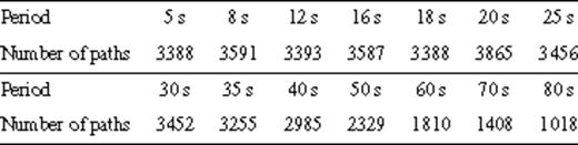
Number of Rayleigh wave group velocity measurements obtained at each period.
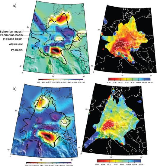
Group velocity maps (left) and the resolution length (right) at (a) 5 s and (b) 16 s. On the resolution maps we show only the area where we have at least 10 paths per cell.
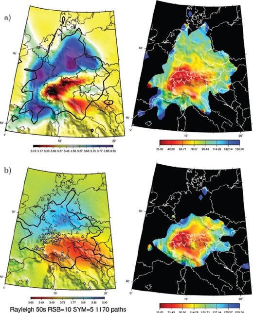
A2 Group velocity maps (left) and the resolution length (right) at (a) 35 s and (b) 50 s. On the resolution maps we show only the area where we have at least 10 paths per cell.
