Green's functions and radiation patterns in poroelastic solids revisited

Summary

1 Introduction

The equations for wave propagation in a fully fluid-saturated porous medium were first proposed by Biot 50 years ago Biot (1956a, b, 1962). Finding solutions of the two coupled poroelastic partial differential equations (PDE) in the presence of body force source terms is an important problem of wave mechanics in porous continua. In particular, if the source term is assumed to be a Dirac's delta function in time and space the solutions are referred to as Green's functions.

Green's functions have been obtained, under various assumptions, by various authors over the last decades. However, the Green's function differ since several combinations of field variables and source terms are possible in a poroelastic continuum. One set of field variables to represent the two PDEs are the solid displacement u and the relative solid-fluid displacement w. Another representation is based on u and the fluid displacement U. The third representation is a combination of a vector and a scalar variable, namely the solid displacement u and the pore-fluid pressure p. Each of these sets of field variables allows different source terms to be introduced. It is therefore not surprising that these different representations lead to a number of publications on Green's function in poroelasticity which are apparently different.

The first authors who derived Green's function for the dynamic poroelastic problem were Burridge & Vargas (1979). Their solution is based on the representation of the poroelastic wave equations using the solid displacement u and the relative solid-fluid displacement w as field variables. Burridge & Vargas (1979) applied the method of potential decomposition in conjunction with the Laplace transform. Explicit solutions were given for the far-field using the saddle point method. As only one type of source, which is a single force vector, is acting on the bulk phase but none on the fluid phase this solution solves the problem only partly. Using the Fourier transform method Norris (1985) derived Green's function in terms of the field variables (u, U). In addition to a source acting on the bulk phase a source vector in the fluid phase was added. In this work no explicit expression of Green's functions including all source types were given. Using a similar approach, Green's functions for poroelasticity were derived by Philippacopoulos (1998) and Lu et al. (2008). Norris (1994) used a different approach based on integration over a closed surface to derive Green's functions for poroelasticity.

Another way to determine Green's function for the equations of poroelasticity is to exploit the analogy with the PDEs of thermoelasticity (Kupradze 1979). This is possible since the PDEs of thermoelasticity and poroelasticity are mathematically equivalent (Norris 1992). The PDEs of poroelasticity can be represented in terms of one vectorial and one scalar field (u, p) (Bonnet 1987). Using the method of Kupradze, the frequency-domain Green's functions were derived by Bonnet (1987) and Boutin (1991). The source term acting on the fluid phase is a volume source V while the source in the bulk composite is a vector force F. In addition to the 3-D space Green's function the solution for the 2-D Green's function was also presented. Bonnet (1987) and Boutin (1991) pointed out that a source vector acting on the fluid phase (as used in Norris 1985) is unphysical.

Green's functions for coupled problem of elastic and electromagnetic wave propagation in porous media were presented by Pride & Haartsen (1996). These solutions can be reduced to the poroelastic Green's functions by neglecting the electromagnetic coupling terms (Müller & Gurevich 2005). On the basis of the field variables (u, w) representation, these Green's functions are given in the frequency space domain and are analogous to those given by Norris (1985). The advantage of the solution presented by Pride & Haartsen (1996) is that Green's functions were presented in the most explicit form separated in far-field and near-field contributions.

All Green's functions described above are presented in the frequency domain. In the presence of the Darcy dissipation term (Biot 1956a, b) it is not possible to analytically transform the results back into time domain without any further assumptions. A closed-form time domain solution for the case without viscous dissipation was given by Norris (1985). Two authors obtained Green's functions in time domain including the viscous dissipation term. Chen (1994a, b) gives solutions for 2-D and 3-D space using the Laplace transform method, however introducing approximations in the Laplace domain. Another approach is presented by Schanz & Pryl (2004) also using inverse Laplace transform method.

The solutions discussed here can be used to implement point sources in a number of seismic forward modelling algorithms in porous media, such as reflectivity (Allard et al. 1986), finite differences (Wenzlau & Müller 2009). The analytical solutions obtained in the paper can be used to benchmark the results of these algorithms. Furthermore, even when the source is physically located in a non-porous region of the medium, such as a fluid-filled borehole, explicit modelling of such geometrical configuration may require a prohibitively small grid size. This problem can be overcome by approximating the borehole as a series of point sources (Kurkjian et al. 1994). This approach requires the computation of the point source response. Thus, the poroelastic point source solutions presented in this paper can also help model the effect of a borehole in a poroelastic formation (including the effect of flow between the reservoir and the borehole).

In this paper, we provide a consistent formulation of Green's functions in poroelastic solids. The similarities and differences between the approaches described above are highlighted. In Section 2, we present the equations of linear poroelasticity. We provide a comparative review of Green's function of poroelasticity in Section 3. Radiation patterns for various source types are illustrated in Section 4. The concept of moment tensors is introduced to describe consistent source mechanisms in poroelastic solids including fluid and solid dipole sources as well as double-couple sources. Their radiation characteristics are also illustrated with the help of radiation patterns.

2 Equations of Poroelasticity

A theory wave propagation in fully saturated porous media was developed by Biot (1956a, b, 1962). The wave equations of dynamic poroelasticity (Biot 1962) can be represented in the frequency domain as

1

2

where w = φ(U−u) is the relative fluid-solid displacement, φ is the porosity, u is the average bulk displacement, and u is the absolute fluid displacement. ρ and ρ_f are the densities of the bulk and the fluid phase where ρ = φρ_f+ (1 −φ)ρ_s, with ρ_s being the density of the grain material.

The viscosity is denoted as η, and the permeability is k. The permeability is frequency dependent and we adopt the dynamic permeability model of Johnson et al. (1987):

3

where the transition frequency ω_t separates the regimes of low-frequency viscous flow and the high-frequency inertial resistance. According to Pride (1994), m is a dimensionless factor describing pore-space geometry, a_∞ is the tortuosity, k₀ is the hydraulic permeability, and Λ, which has the dimension of length, represents a weighted volume-to-surface ratio. m lies between 4 ≤ m ≤ 8. In the low-frequency limit, expression (3) reduces to the hydraulic permeability k₀.

σ and p are the total stress tensor and fluid pressure, which are related to the displacement vectors via the constitutive relations

4

5

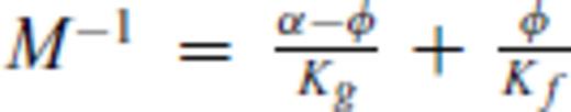In eqs (4) and (5)μ is the shear modulus of the solid frame, α = 1 −K/K_g is the Biot–Willis coefficient (Biot & Willis 1957), is the so-called pore space modulus and the saturated P-wave modulus is defined by H = K_sat+ 4/3μ. K_sat is the bulk modulus of the saturated medium that is related to the bulk moduli of the fluid K_f, solid K_g, and dry skeleton K by the Gassmann (1951) equation

6

Eqs (1)–(6) constitute the framework of wave propagation in fluid-saturated porous solids. To obtain Green's functions, appropriate source terms have to be introduced in eqs (1) and (2).

3 Green's Functions in Poroelasticity

In elastodynamics, the Green's function approach is commonly used. The representation theorem of elastodynamics relates the displacement field ũ, excitation force , and Green's function in time domain (Aki & Richards 2002) in the form of a convolution

7

This equation can be expressed in the frequency domain as

8

Using eq. (8), it is possible to compute the displacement field for any point and any frequency for arbitrary excitation. For further properties of Green's function in elastodynamics, we refer to the textbook of Aki & Richards (2002).

A similar approach can be used to derive Green's function for poroelasticity. Eqs (1), (2), (4) and (5) can be represented as a pair of coupled wave equations by inserting the constitutive relations (4 and 5) into the equations of motion (1 and 2). However, depending on which of the three field variables (u, w or p) is eliminated, the set of wave equations consists of either six or four wave equations. Choosing u and w as field variables, one obtains two vector wave equations, whereas choosing u and p one obtains one vector and one scalar wave equation. Introducing source terms into these sets of equations allows to derive Green's functions that are different for both sets of equations. These two different Green's functions are reproduced in the next section based on the work of Pride & Haartsen (1996) and Boutin (1987).

3.1 Solid and relative fluid-solid displacement representation

To obtain wave equations for the homogeneous and isotropic poroelastic wholespace including the solid and relative displacement (u, w) as field variables the stress tensor σ_ij and the pore pressure p have to be eliminated from the governing eqs (1) and (2). By substituting eq. (4) into eq. (1) and eq. (5) into eq. (2), we obtain the following matrix differential equation:

9

where L_u,w is the matrix differential operator

10

In this equation is

11

and I is the identity tensor. Time dependence is assumed as exp(−iωt). Source terms in the form of body forces F and f are introduced on the right-hand side, which act on the bulk and the fluid phase, respectively. Assuming source terms in the form of Dirac delta functions

12

13

where r′ is the location vector pointing to the source position and r indicates the observation point, a solution of eq. (10) involving the corresponding Green's tensors can be expressed as

14

Green's tensor G^F,u describes the solid displacement u response due to a bulk force F₀ excitations. G^f,w describes the relative displacement w due to a force F₀ acting on the fluid phase. The other Green's tensors can be interpreted in a similar way.

Explicit expressions for these Green's tensors can be obtained using the Fourier transform method. To do so, eq. (9) is transformed into the spatial wavenumber domain resulting into a system of six algebraic equations. This system of equations can be solved for Green's tensors in frequency-wavenumber domain. The spatial response can be obtained by applying the inverse Fourier transform in spherical k coordinates. This yields (Pride & Haartsen 1996):

15

In eq. (15), the Green tensors are separated in components with transverse , longitudinal and near-field polarizations; is the unit direction vector pointing from the source to the observation point. and are the amplitudes of the transverse and longitudinal components. They are specified through the type of source indicated by ξ = {F, f} and the type of field indicated by η = {u, w} and the slownesses of the fast and slow compressional waves, s₁, s₂, and the shear wave, s₃. Explicit expression of these three wave slownesses is given in Appendix A. The expressions for the amplitudes and is given in Appendix B. Green's functions as defined in (14) and (15) can be easily reduced to the elastodynamic Green's function. In this case, only Green's function G^F,u exists since in an elastic solid only the solid displacement field u due to a body force vector F₀ is excited. Then, in eqs (15) one has to set the slow P-wave slowness to zero.

Eqs (15) are equivalent to the fundamental solutions provided by Norris (1985). The solution from Norris (1985) was considered by Bonnet (1987) as overdetermined as a scalar source term is sufficient to describe sources in the fluid phase. Such a solution was derived by Boutin (1987) and is outlined in the next section.

3.2 Solid displacement and pore pressure representation

The correspondence between thermoelasticity and poroelasticity was pointed out by Norris (1992). In particular, the pore-fluid pressure is the poroelastic counterpart of the temperature as scalar field variable in thermoelasticity. Eliminating the stress tensor and the relative displacement vector w from eqs (1), (2), (4) and (5) results into a vector wave equation for the solid displacement vector u and into a scalar wave equation for the pore-fluid pressure

16

with the matrix differential operator L_u,p defined as

17

ρ_t and are defined as

18

The dry P-wave modulus is defined as P_dry = K+ 4/3 μ. In eq. (16), two source terms are introduced, where F is a body force acting on the bulk phase (the same as in eq. 8), while the scalar source term V corresponds to a volume injection applied within the fluid phase. Assuming that these sources have the form of Dirac delta pulses

19

20

eq. (16) can be represented with help of eq. (8) in terms of Green's functions

21

As in eq. (14), four Green's tensors appear, however, their structure is different. The solid displacement response u due to a body force vector on the solid phase F₀ is a tensor of rank 2, G^F,u. The pressure response p due to the same force and the displacement response due to a volume injection source are vectors, G^F,p and G^V,u. Finally, Green's function connecting the scalar source V to the fluid pressure p is of scalar nature, G^V,p.

The problem of determining Green's functions can be solved in analogy to thermoelasticity by using the method of Kupradze (1979, pp. 94). This method can be summarized as follows (a detailed outline of the method is also given in Sahay (2001, Section 4.1). The impulse response can be obtained by solving

22

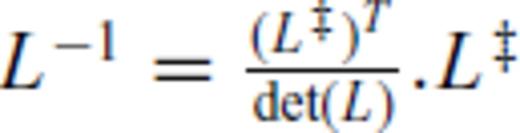where L⁻¹ is the inverse of the differential operator in eq. (17), which can be represented as is the cofactor matrix of L and τ is the solution of the scalar equation .

The (u, F) response G^F,u is identical to that of eq. (15). Due to the symmetry of eq. (21) Green's functions G^V,u and G^F,p are the same. This means that the displacement response u due to a volume source V and the pressure response p due to a single force vector F can be expressed as

23

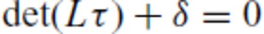where η = {u, p} and ξ = {V, F}. The amplitudes are given in the Appendix B. It is interesting to observe that the pressure field can be separated into a far-field term (first term proportional to 1/r) and a near-field (first term proportional to 1/r²). The scalar Green's function describing the pressure response p due to a volume source V is

24

where the amplitudes are listed in the Appendix B.

Green's tensors (15), (23) and (24) fully describe a poroelastic medium as they provide solutions for all possible combinations of field variables (u, w, p) and for all possible forces (F, V). Note, however, that the single force in the fluid f is an unphysical source, as a fluid can only sustain hydrostatic pressure. This was already pointed out by Bonnet (1987).

Below we show that this inconsistency can be overcome by introducing the concept of moment tensor sources, thus replacing the single body force in the fluid phase by the body force equivalent of an explosive source.

4 Radiation Patterns

The radiation characteristics of waves emanating from various sources in poroelastic continua have only been investigated by Molotkov & Bakulin (1998). However, their work is restricted to the high-frequency range of Biot's theory. We generalize this work by analysing radiation characteristics in the full frequency range for relevant source configurations. A useful way to present the radiation characteristics of sources in elastic continua is presented by Chapman (2004). Here we follow this approach to construct radiation patterns of sources in poroelastic continua.

Radiation patterns show the directional behaviour of the displacement magnitude ǀu ǀ generated by different source configurations. For a fluid-saturated porous medium the field variables can be either solid displacement u, relative displacement w or pore pressure p. Based on eq. (8) all Green's functions of poroelasticity can be represented in terms of field variables in the generic form

25

where u^P,S represents the displacement of the longitudinal (P) or shear (S) waves. The right-hand side of eq. (25) consists of the scalar product of the source excitation (either body force F or injection volume V) and the polarization (one of ) multiplied by the corresponding amplitude

26

where L, T are defined in the Appendix B. Similarly, the scalar response p can be represented as

27

where

28

The right-hand side of eq. (27) represents the possible combinations of polarizations and source terms that produce a fluid-pore pressure field.

4.1 Point force source

4.1.1 Far-field

According to eq. (25) and Chapman (2004, Sec. 4.5.5.1) the P-wave radiation pattern is given by . Using spherical coordinates, the unit vector can be expressed as

29

where θ and κ are the angles from the z and x axes, respectively. The radiation pattern for the P wave is then

30

The S-wave radiation pattern is constructed as follows. The unit basis vectors of the spherical coordinate system satisfy the identity

31

Thus, the S-wave polarization can be expressed as . The polarization of the S wave is in the plane perpendicular to the propagation direction . If the z-axis is vertical, and the x−y plane is horizontal, it is common to introduce the notion of SH and SV waves. The horizontal component is

32

yielding the radiation pattern of a SH wave

33

The vertical component can be expressed as

34

From eq. (34) we get the radiation pattern of a SV wave as

35

Assuming a body force with z component only, i.e., F = (0, 0, F_z)^T acting on a poroelastic solid, the radiation patterns of the solid displacement u and relative solid-fluid displacement are illustrated in Figs 1–3 using the frequency of 100 Hz and the material parameters as specified in Table 1. It can be observed that the shape of the radiation patterns is identical to the elastodynamic case. The P-wave displacement is largest in the direction of the applied force, whereas the S-wave displacement is largest perpendicular to the direction of the force vector. The amplitude of the S wave is larger than that of the P wave. In addition, the radiation pattern of the slow P wave has the same shape as that of the fast P wave, however its amplitude is significantly smaller (its amplitude has been amplified by a factor 10⁸ to make it visible in Fig. 1).

Figure 1.

Radiation pattern of solid displacement u due to a point force; the numbers 2 × 10⁻¹² to 6 × 10⁻¹² denote the displacement in meters along the radial axis; the radiation pattern of the slow P wave is enhanced by the factor 1 × 10⁸.

Open in new tabDownload slide

Figure 2.

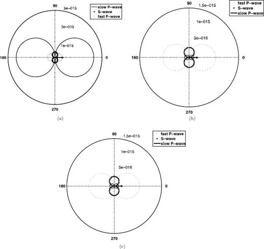
Radiation pattern of fluid displacement U due to single force for slow P wave, fast P wave and S wave, respectively; the numbers along the radial axis denote the displacement in meters; results are given for three different frequencies (a) 15 Hz, (b) 25 Hz, (c) 100 Hz.

Open in new tabDownload slide

Figure 3.

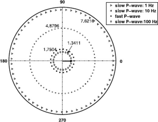
Pressure field p due to a single force F for the slow and the fast P wave; the numbers 1.7504–7.6216 denote the pressure in Pascal along the radial axis; The slow P-wave dispersion is illustrated for three frequencies: 1 Hz, 10 Hz and 100 Hz.

Open in new tabDownload slide

Table 1.

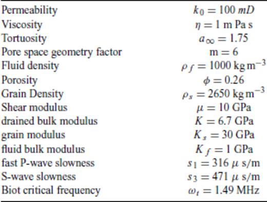
Material parameters of a typical sandstone used for the computations.

Open in new tabDownload slide

As a poroelastic medium is a two-phase system, the two P waves are differently manifested for different field variables. Comparing Figs 1 and 2(c) showing the solid and fluid displacement for 100 Hz, respectively a difference in magnitude of factor 4 from solid to fluid displacement can be observed. The slow P wave is easier to observe in terms of the fluid displacement especially for smaller frequencies (Figs 2a and b). Here the contribution of the fast P wave and S wave becomes significantly smaller than the slow P-wave displacement.

In Fig. 3, the pressure response p due to a single force F acting in z-direction (compare eq. 23) is computed for various frequencies. In this case only the fast and slow compressional waves exist. The values computed are plotted on a logarithmic scale. For low frequencies, the slow P wave (1-10 Hz) has a bigger amplitude than the fast P wave. For higher frequencies, the slow P-wave amplitude decays rapidly. An analogous case is the pressure field due to a volume source (eq. 24). The difference is that the slow P-wave amplitudes are larger while the fast P-wave amplitudes are smaller. The low-frequency limit of this case was studied by Chandler & Johnson (1981), Rudnicki (1986) and Müller (2006).

4.1.2 The near-field

At distances smaller than one wavelength the near-field terms become noticeable (Wu & Ben-Menahem 1985). The polarization of the near-field is and the leading-order amplitude decays as 1/(ωs_ir²) (while the far-field decays with 1/r). Using again identity (31), the near-field polarization can be expressed as

36

Assuming a force acting in z-direction and using eqs (29), (34) and (32) we find the near-field polarization

37

The radiation pattern of the near-field is illustrated in Fig. 4. The form is the same for elastic and poroelastic media, only the amplitude differs. In source direction the amplitude is smaller than in perpendicular direction. This already indicates the difference in amplitude of P waves and S waves. Looking at eq. (23) it is obvious that the second term also decays like near-field terms but has the same polarization as the far-field. This means that for a pressure field due to a force vector (or displacement due to volume source) part of the energy decays with 1/r² but with the same directivity as the far-field.

Figure 4.

The radiation characteristics of the near-field. Only the geometry is illustrated without rock parameters.

Open in new tabDownload slide

4.2 Moment tensor sources

Single body forces, as presented in the previous section are often not sufficient to describe real physical sources. For example, if a seismic vibrator or a hammer is used as a source acting on the surface of a poroelastic solid, a single body force representation is sufficient. However, as isolated forces cannot exist inside a closed system (e.g. the earth), it is necessary to introduce the concept of moment tensors (Backus & Mulcahy 1976a, b). The concept of moment tensors is widely acknowledged in elasticity (Aki & Richards 2002; Rudnicki & Freund 1981). In earthquake seismology they are used to describe dislocation type sources. Moment tensors are used as well to describe explosive/pressure sources and higher order type of sources such as dipoles. Such source types are mostly used in exploration seismology and borehole acoustics. The displacement field can be expressed in frequency domain as

38

This means that in the frequency domain the displacement field can be computed as a product of the spatial derivative of Green's function and the moment tensor M_jk. The components of the moment tensor in form of its equivalent body forces are illustrated in Fig. 5 (Aki & Richards 2002). A review on the use of moment tensors can be found in Jost & Herrmann (1989).

Figure 5.

Body force equivalents of the moment tensor components (after Aki & Richards 2002).

Open in new tabDownload slide

A similar approach can be used to study moment tensor sources in poroelastic media. To use moment tensor sources, expressions eqs (25) and (27) have to be modified accordingly

39

where an additional multiplication with the slowness s_j appears as a consequence of the spatial derivative in eq. (38). On the left-hand side, the field quantity can be either a displacement (u, w) or the pressure p. The components of the moment tensor are

40

From eq. (40) and Chapman (2004, Sec. 4.6.2), we deduce that the radiation pattern of moment tensor sources for P waves is . Introducing spherical coordinates yields

41

In analogy to the body force source we obtain the SV radiation pattern by substituting eq. (34) into yielding

42

The radiation pattern for SH waves is using eq. (32)

43

These expressions allow to construct various moment tensor sources such as explosive, dipole and double-couple sources as exemplified next.

4.2.1 Monopole source

An explosion source can be represented by an isotropic moment tensor of the form

44

Introducing eq. (44) into eq. (14) allows to generate physically realizable sources in the fluid phase. The fluid phase cannot sustain a single force vector f, however, substituting the isotropic moment tensor M_ij = M^f₀δ_ij into eq. (14) yields

45

46

The two terms including sources acting on the solid phase G^F,u and G^F,w support the full moment tensor while those terms containing source vectors in the fluid phase (G^F,w and G^F,u) only support an explosive source with magnitude M^f₀. In other words, due to the use of moment tensors a physical meaning is given to Green's functions (14), which support force vectors in the fluid phase.

4.2.2 Dipole source

A dipole source can be realized either in the solid or in the fluid phase. In the solid phase, it can be thought of as tensile stress on a fault surface. Assuming the fault surface to be the x−y plane, yields a momentless force couple acting along the z-axis expressed in terms of moment tensors as (Chapman 2004)

47

The P-wave radiation pattern is then obtained by setting corresponding terms in eq. (41) equal to zero. We obtain for the P-wave radiation pattern

48

and for the SV wave using eq. (42)

49

The radiation patterns for a dipole source acting on the bulk are illustrated in Figs 6–9. Fig. 6 gives a qualitative impression how a dipole source radiates into 3-D space. The P-wave radiation pattern in Fig. 6(a) has a similar form to its equivalent for a single force vector, however, its cones are more directionally shaped. The S-wave radiation in Fig. 6(b) of a dipole source are two doughnuts with zero radiation in axial direction. Both radiation patterns are symmetric with respect to the force direction.

Figure 6.

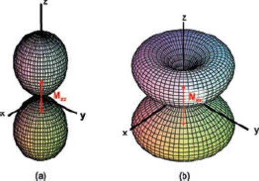
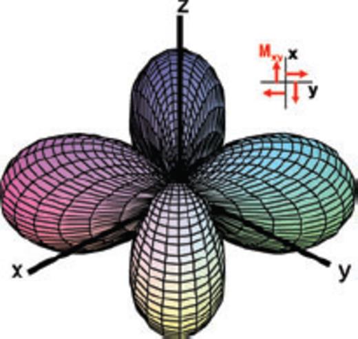
(colour online) Geometry of a 3-D radiation pattern for a dipole source acting on the solid phase; (a) P wave (b) S wave.

Open in new tabDownload slide

Figure 7.

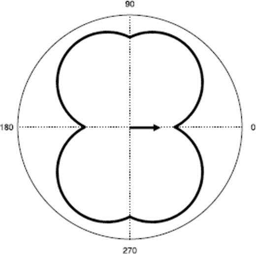
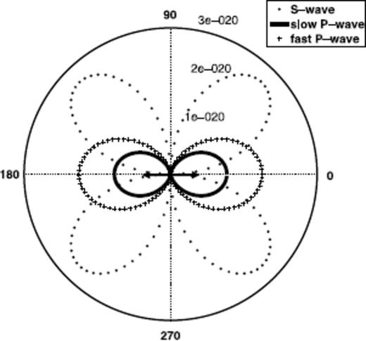
Dipole radiation pattern for solid displacement u; the numbers denote the displacement in meters along the radial axis; Cross-section perpendicular to the x-y plane; the slow P-wave radiation pattern is amplified by factor 3 × 10⁵.

Open in new tabDownload slide

Figure 8.

Dipole radiation pattern for the relative displacement w; the numbers denote the displacement in meters along the radial axis; Cross-section perpendicular to the x-y plane.

Open in new tabDownload slide

Figure 9.

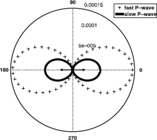
Dipole radiation pattern: pore pressure p; Cross-section perpendicular to the x-y plane; the numbers 5 × 10⁻⁵ to 0.00015 denote the pressure in Pascal along the radial axis; the slow P-wave displacement is amplified by factor 2 × 10²; no shear wave is radiating in the fluid phase.

Open in new tabDownload slide

Figs 7–9 give a quantitative interpretation of a dipole source acting on a poroelastic medium. The responses for a medium described by the parameters in Table 1 are computed in terms of the solid displacement u, the relative displacement w and the pore pressure p. Similar to the single force case it can be observed that the solid displacement response is stronger by a factor of 5 compared to the relative displacement. The slow P wave is amplified by a factor of 3 ×10⁵ for the solid displacement while it is not amplified for the relative displacement. Obviously, the slow P wave is stronger emphasized for w even though the overall magnitude is smaller. The strongest response for both P waves can be observed in the pressure field. The slow P wave is amplified by a factor of 3 × 10⁵ but still has a significantly larger amplitude than for u and w.

4.2.3 Fluid dipole source

As a source in the fluid phase can only consist of a volume source that can be either a volume injection V or an explosion, the fluid dipole source cannot be represented by the moment tensor concept. To overcome this difficulty, we use the concept introduced by Wang (2000) (section 5.8). A dipole source acting on the fluid phase can be thought of as a fluid sink distribution and a fluid source distribution displaced by vector d. The pressure field can be expressed as

50

This means that the pressure field of a dipole is the negative directional derivative of a pressure field due to a volume point source multiplied by the distance of the source and the sink. Using eq. (21) the pressure field (50) can be written as

51

Computing the gradient of both sides of eq. (24) yields the pressure field for a fluid dipole due to a pair of volume source and sink. Using the parameters from Table 1, the radiation pattern of such a dipole is illustrated in Fig. 10. The distance is assumed as ǀd ǀ = 1 m and the orientation of the dipole is along the z-axis.

Figure 10.

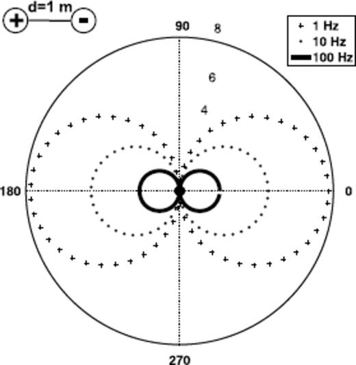
Fluid dipole radiation pattern: logarithm of the pore pressure p of the slow P wave for three frequencies; the numbers 4 − 8 denote the pressure in Pascal along the radial axis; point in the centre is the fast P wave that is negligibly small compared to the slow P wave.

Open in new tabDownload slide

4.2.4 Double-couple source

Another source type that can be described using moment tensors is a double-couple source. For a fault in the x−z plane with slip in x-direction the moment tensor is reduced to its off-diagonal components

52

Eq (41) for the P-wave radiation pattern reduces then to

53

Its 3-D radiation is qualitatively illustrated in Fig. 11. It has the form of a four-leaved clover with maximum energy radiated in the x−y directions and zero energy in the direction of the coordinate axes. Two diagonal lobes are rotationally symmetric with respect to x = y.

Figure 11.

(colour online) 3-D P-wave radiation pattern of a double-couple source.

Open in new tabDownload slide

The SH-radiation pattern in the x−y plane is

54

The 3-D radiation pattern (Fig. 12a) is again a four-leaved clover but it is rotated by 45° with respect to the z-axes. For the SV wave, the radiation pattern is given by

55

and is illustrated in Fig. 12(b). It has eight lobes, one in each quadrant radiating maximum energy in the diagonal direction. The radiation patterns of a double-couple source are also illustrated in Figs 13–15.

Figure 12.

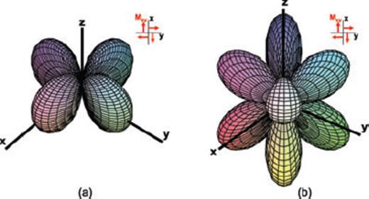
(colour online) 3-D radiation pattern of a double-couple source; (a) SH wave (b) SV wave.

Open in new tabDownload slide

Figure 13.

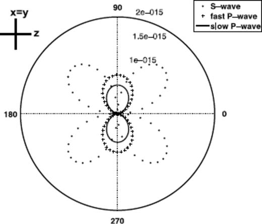
Double-couple radiation pattern: solid displacement u; the numbers 1 × 10⁻¹⁵ to 2 × 10⁻¹⁵ denote the displacement in meters along the radial axis; the slow P wave displacement is amplified by 5 × 10⁵.

Open in new tabDownload slide

Figure 14

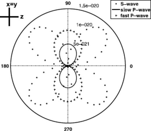
Double-couple radiation pattern: relative displacement w; the numbers 5 × 10⁻²¹ to 1.5 × 10⁻²⁰ denote the displacement in meters along the radial axis.

Open in new tabDownload slide

Figure 15.

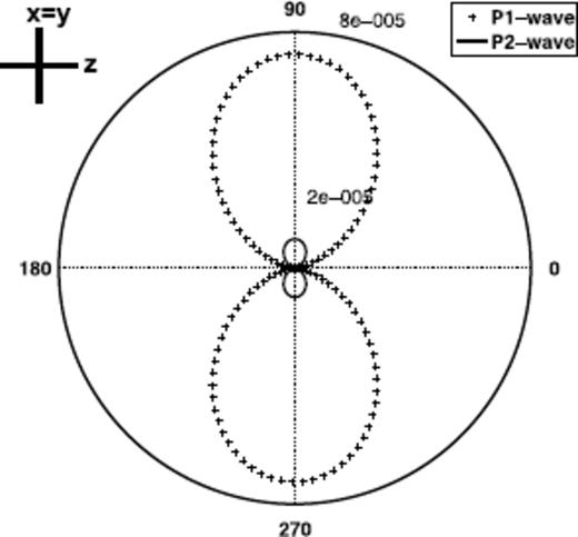
Double-couple radiation pattern: pore pressure p; the numbers 2 × 10⁻⁵ to 8 × 10⁻⁵ denote the pressure in Pascal along the radial axis; the slow P-wave radiation pattern is amplified by 1 × 10⁵.

Open in new tabDownload slide

5 Conclusions

A review and comparison of different formulations of Green's functions for dynamic poroelasticity is provided. We conclude that previously reported sets of Green's functions can be used in a complementary sense such that all possible combinations of field variables and source types are included. We think that the unified presentation of Green's functions resolves the apparent contradictions between existing formulations. As expected, the shape of the radiation patterns of the fast compressional and shear wave is identical to their elastodynamic counterparts, however, complemented with the radiation pattern of Biot's slow wave. The relative magnitudes of the field variables shown in the radiation patterns can be very different for different source types. In particular, for any source acting in the fluid phase the pressure field is dominated by the Biot slow wave having compressional wave polarization. We introduce the concept of moment tensors for dynamic poroelasticity that allows us to overcome the inconsistency in Green's function formulation with respect to point force sources in the fluid phase.

Acknowledgments

We thank A. Bakulin (WesternGeco, Houston) who suggested to work on this topic at hand. The work of TMM was kindly supported by the Deutsche Forschungsgemeinschaft (contract MU1725/1-3).

References

Appendices

Appendix A: Biot Bulk Wave Slownesses

The bulk wave slowness in a poroelastic medium is given by

(A1)

where s₁, s₂ and s₃ are fast, slow compressional and shear slowness respectively and C = αM. The coefficient γ is defined as

(A2)

Appendix B: Amplitudes of Green's Functions

The amplitudes appearing in the expression for the Green tensors (15), (23) and (24) are given by

(B1)

Author notes