A method of fast, sequential experimental design for linearized geophysical inverse problems

Summary

1 Introduction

In exploration geophysics, standardized or ad hoc surveys cannot guarantee optimally informative data sets; that is, data sets whose inversions assure high model accuracy or minimal model uncertainty. For an arbitrary heterogeneous target, it is reasonable to conjecture that there exists an ideal survey that optimizes the information content of the data and that standard survey geometries must almost certainly be suboptimal in comparison.

The deliberate, computational manipulation of geophysical surveys in order to create data with superior information characteristics is termed optimal experimental design (OED). Tangentially, the terms survey and experiment will be used interchangeably. OED is distinguished principally by the fact that it treats design as a computational problem, and its prime objective is to create compact sets of observations that produce superior data quality. Thus, experimental design seeks to maximize the connection between the data collected and the model from which they derive.

Geophysical constitutive equations are (typically) non-linear functions that can be cast in terms of a forward operator g that maps a model m to data d by means of an observation at ω, viz.,

1

A set of observations,

2

constitutes an experiment, which governs collection of the data set; the set of all experiments is experiment space; the set of all data corresponding to individual observations is data space; and the set of all earth models is model space. Each experiment can be quantitatively ascribed a ‘quality metric’ indicating how strongly it informs the connection between data and model space, and the object of the designer is to search experiment space for the highest quality mapping between data and model space.

This article examines linear or linearized experimental design, which proceeds from the linearization of eq. (1):

3

where G is the sensitivity (Jacobian) matrix, comprising the M×D partials of g(m, ω_i) with respect to the discretized model parameters m_j:

4

The Jacobian and its inverse, G and G*, respectively, are the objects upon which linearized experimental design typically operates (e.g. Atkinson et al. 2007). Curtis & Spencer (1999) and others have pointed out that because eq. (3) is a linear approximation, it is valid only in the neighbourhood of the Taylor expansion point in model space, implying that G is only technically valid in this neighbourhood. If G depends on m, and the design objective function operates on G, then the experimental design depends on m. For non-linear inverse problems, an experimental design should ideally be optimal with respect to the true solution and with respect to all points in model space through which the inversion passes on its trajectory to the true solution. Approaches to the fully non-linear design problem can be found in the literature on Bayesian experimental design methods (e.g. Sebastiani & Wynn 2000; van den Berg et al. 2003) and in novel methods for reducing non-uniqueness in non-linear problems (Winterfors & Curtis 2008), but this article does not delve into these. Instead, linearized design theory is adopted because its methodologies are currently more practicable, though less general, than non-linear experimental design. However, we introduce an adaptive design procedure that benefits from the expedience of linearized design, potentially circumventing the computational complexity of non-linear design.

The chief problem with geoscientific survey design is computational expense. There have been two reasons for this: first, design is a challenging combinatorial optimization problem (Haber et al. 2008); second, many of the proposed design objective functions are expensive to calculate. With regard to the former, Curtis (1999a), Maurer et al. (2000), Barth & Wunsch (1990) and others have used global search algorithms like the genetic algorithm, simulated annealing, etc. to find critical points of their design objective functions. Such algorithms are ideal for combinatorial optimization problems like experimental design, but they are too slow to be practical for many real problems. There is however an exceptional class of fast algorithms - so-called greedy algorithms- that forms the basis for the design methods introduced in this work. More is said about these later.

Nearly all geoscientific design objective functions operate on G or G*, as pointed out above (Barth & Wunsch 1990; Rabinowitz & Steinberg 1990; Maurer & Boerner 1998a, b; Curtis 1999a, b; Curtis & Spencer 1999; Curtis & Maurer 2000; Maurer et al. 2000; Stummer et al. 2002, 2004; Friedel 2003; van den Berg et al. 2003; Curtis et al. 2004; Furman et al. 2004; Narayanan et al. 2004; Routh et al. 2005; Wilkinson et al. 2006a; Furman et al. 2007). These objective functions are readily understood in terms of the eigenspectra of G (Curtis 1999a, b), and indeed many proposed objective functions explicitly operate on the eigenspectrum (Barth & Wunsch 1990; Curtis 1998; Maurer & Boerner 1998a; Curtis 1999b; Maurer et al. 2000). However, Maurer et al. (2000) point out that eigen-analysis takes O(N³) operations, making it computationally expensive. Even for objective functions that do not require eigen-analysis but operate indirectly on eigenvalues through the trace or determinant of (G^TG)⁻¹ (Kijko 1977; Rabinowitz & Steinberg 1990; Maurer et al. 2000; Narayanan et al. 2004), the computational complexity still remains high, owing to the expense of inverting G^TG and/or taking its determinant.

Mindful that computational expense has been a hindrance to practical OED, this paper introduces an efficient sequential design technique inspired by the works of Stummer et al. (2002, 2004), Wilkinson et al. (2006a) and Curtis et al. (2004). This approach is an example of greedy optimization (e.g. Papadimitriou & Steiglitz 1998), which trades global optimality for faster computation times. The well-known design objective function is used throughout, and, critically, this function is made computationally efficient through the use of special update formulae. Additionally, a simple, adaptive design procedure is introduced that may serve as an alternative to (currently) impractical non-linear design methods and which can be employed in near real time. We demonstrate the methods on a synthetic single-borehole DC resistivity problem. While the chosen example is somewhat artificial, we emphasize that the paper is on survey design and this example does not detract from that focus.

2 Methods

2.1 The OED objective function and update formulae

A common objective function in experimental design theory, and the one used in this article, is

5

which is minimized over the space of possible experiments (Box & Lucas 1959; Rabinowitz & Steinberg 1990; Steinberg et al. 1995; Sebastiani & Wynn 2000; Narayanan et al. 2004). Since , the design problem can also be expressed as the maximization problem,

6

where Ω is the space of all possible experiments. The stationary point(s) of eq. (5) have been shown to minimize the model entropy (Sebastiani & Wynn 2000; van den Berg et al. 2003) or the volume of model uncertainty (Narayanan et al. 2004), which are mathematically equivalent measures of global model uncertainty for linearized problems. Below we develop a novel approach for finding quasi-stationary points of eq. (5) without the need to directly calculate expensive determinants or matrix inverses.

2.1.1 Rank-one updates toand

This section establishes update formulae for rapidly evaluating or when rows are added to A. This anticipates the situation where observations are sequentially added to an existing experiment, which corresponds to adding rows to the Jacobian matrix. Proofs for all update formulae here can be found in the Appendices.

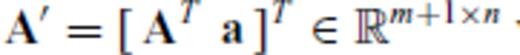
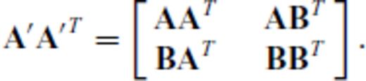
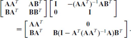
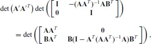
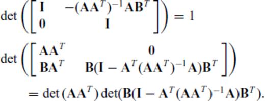
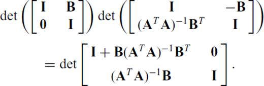
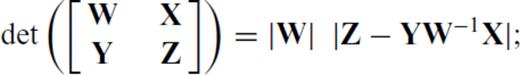
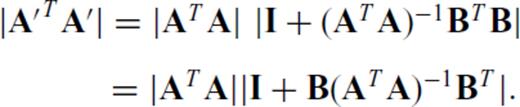
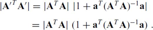
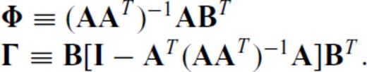
Given a block matrix , where , and m+p ≤ n, the determinant of A′ A′^T is given by

7

Dividing by and substituting a^T for B (i.e., p = 1) yields

8

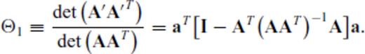
If m+p > n, the update for is

9

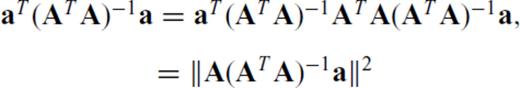
Dividing by , substituting a^T for B and manipulating terms yields

10

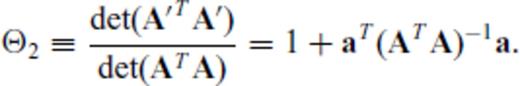
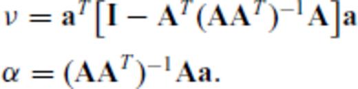
Because and are assumed known and fixed, maximizing Θ₁ or Θ₂ with respect to a satisfies the design criterion in eq. (6). The utility of this fact is made clear in Section 2.3, when the design algorithm is developed. Importantly, eqs (8) and (10) involve only matrix-vector products, which are computationally more efficient than explicitly evaluating determinants and inverses.

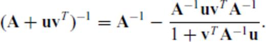
2.1.2 The Sherman-Morrison formula

The Sherman-Morrison formula (SMF) is an identity relating the inverse of a matrix to the inverse of its rank-one update. Formally, the SMF states

11

The SMF provides a computationally inexpensive way to update a matrix inverse without resorting to a full inverse calculation. Let where , and m+ 1 ≥ n. If A^TA is invertible, then

12

Since (A^TA)⁻¹ is assumed known, evaluating (A′^TA′)⁻¹ requires only a few matrix-vector products, which is more efficient than performing the full numerical inverse.

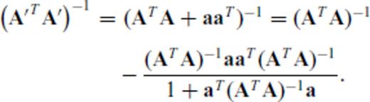
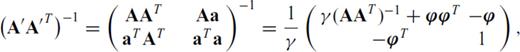
The situation is more complicated for A′A′^T. If AA^T is m×m, then A′ A′^T is . The object is to relate the inverses of two matrices of different dimensions. It is straightforward to show that

13

where

14

Eq. (13) provides a way to evaluate (A′ A′^T)⁻¹ cheaply, by avoiding a full inverse computation.

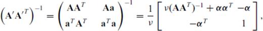
Collectively, the Sherman-Morrison and determinant update formulae provide an efficient way to quickly find observations satisfying eq. (6) without explicitly evaluating inverses or determinants. These formulae will be critical for the speed of our design algorithms introduced below.

2.2 OED considerations for DC resistivity

In practice, four electrodes are needed to make any single DC resistivity measurement, two as the source dipole and two as the receiver dipole. Noel & Xu (1991) and others (Xu & Noel 1993; Daily et al. 2004; Stummer et al. 2004) have proven that, for any resistivity survey of N geoelectrodes, there are a total of

15

four-electrode observations available for experimentation, accounting for reciprocity and polarity switching. Noel & Xu (1991) have further shown that the maximum number of independent measurements is

16

That is, if one has identified a set of S_N independent resistivity observations, then any other observation can be expressed as a linear combination of these. If N = 20 geoelectrodes, for example, there are 14 535 possible four-electrode measurements but only 170 of these are independent. This is one of the reasons why resistivity inversion is nearly always non-unique: the amount of potential information a survey can offer is far smaller than is suggested by the number of available observations.

Considering a generic linearization of the DC resistivity forward problem,

17

the fact that there are at most S_N independent observations means that the maximum attainable rank (MAR) of G cannot exceed S_N:

18

In other words, G can never have more than S_N non-zero singular values. This concept is examined in Section 2.3.1.

2.3 Basic OED algorithm

Before describing the new design algorithm, an important detail should be pointed out. The eigenvalues of G^TG and GG^T are identical up to zeros. Because the determinant operates on these eigenvalues (it equals their product), G^TG and GG^T effectively convey the same information about the quality of a survey, but in two different ways. The reason update formulae are given for inner and outer products is because in the early stages of the algorithm, there will be fewer observations than model parameters, so GG^T will be full rank while G^TG will not; in later stages, G^TG will be full rank while GG^T will not. Because their eigenvalues are the same, the trick will be to use GG^T when the design problem is ‘underdetermined’ and G^TG when it is ‘overdetermined’. This avoids zero eigenvalues which could render a determinant-based objective function useless.

Geoelectrical inverse problems are almost never full rank, however, and special consideration is made to accommodate this in Section 2.3.1. Nevertheless, the purpose of this paper is to introduce a design technique useful for a wide class of problems, so the main algorithm is introduced first and specific modifications for geoelectrical problems are discussed afterward.

The following nomenclature is used in the basic OED algorithm:

Open in new tabDownload slide

Basic sequential OED algorithm:

• 1

  Set k = 1 and find the observation in whose sensitivity kernel, g, is of maximum length (note: , so eq. 6 is satisfied). Set G_b = g^T.

• 2

  If , update (G_bG^T_b)⁻¹ using SMF; if , evaluate (G^T_bG_b)⁻¹ explicitly; else if , update (G^T_bG_b)⁻¹ using SMF.

• 3
  If use eq. (8) to evaluate the candidacy of observations in for transferal to . Eq. (8) can be efficiently executed by

  

  Else if , use eq. (11), which can be efficiently executed by

  

  Note that .
• 4

  Identify the winning candidate in that maximizes either or and transfer it to .

• 5

  Set where g is the sensitivity kernel in G_M corresponding to the winning candidate observation identified in step 4.

• 6

  Increment k arrow k+ 1.

• 7

  Stopping criterion, e.g. if k is less than some desired number of observations, go to 2; else exit.

The algorithm described above is plainly sequential; it proceeds by identifying the best observation to add to an experiment (conditional on the observations already in the experiment), adding it, and repeating until a stopping criterion is met. This formulation allows for repeat observations in the survey design, but it can easily be modified if this is undesirable. This is an example of a greedy algorithm (e.g. Papadimitriou & Steiglitz 1998), which is a method of optimization that proceeds by making locally optimal updates to a solution given the solution currently at hand. Only under strict circumstances can greedy optimization algorithms give rise to globally optimum solutions, which is largely due to the fact that they do not exhaustively search the entire space of possible solutions. The utility of such algorithms lies in the fact that they execute far more quickly than global optimization algorithms. The question is: does the value gained in computing efficiency offset the value lost in deviation from a globally optimum experiment? We look at this question later in our synthetic examples.

2.3.1 Maximum attainable rank

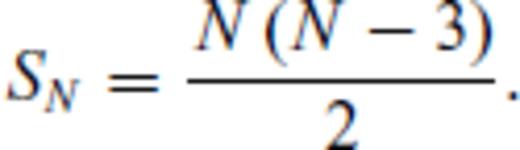
Section 2.2 raised the possibility that the inverse problem is inherently ill posed, meaning the model parameters cannot be fully resolved, no matter what is the number of data observations. The MAR, denoted , defines the highest rank any row-deleted submatrix of G_M can attain, which is plainly

19

Special care is needed in survey design when the inverse problem is inherently ill posed, which happens if ζ <. In such cases, any row-deleted submatrix, G_b of G_M, that has more rows than the MAR must also have non-trivial left and right null spaces and hence . This makes Θ₁ and Θ₂ both degenerate (they vanish or become indeterminate), rendering them useless in our algorithm.

There are a number of ways of dealing with this problem; here, we focus on a form of information compression via singular value decomposition (SVD). If it is unknown a priori that the inverse problem is inherently ill posed, it shall become apparent when Θ₁ goes to zero for all candidate observations before the number of observations in the base experiment reaches . This is because Θ₁ is maximized at each design step, so must be non-negative and vanishes only if ζ < . In fact, it should be clear Θ₁ automatically vanishes for all candidate observations at iteration ζ+ 1, when the number of observations exceeds the MAR by one.

To circumvent this problem, we use the SVD of G_M,

20

where G_M has ζ non-zero singular values. G_M can be exactly expressed by its truncated singular value decomposition,

21

such that , and . We transform G_b and G_M by right multiplication with to produce

22

so that the number of columns in G′_b and G′_M is now ζ (). Critically, is an isometric projection operator - it maps points in model space to a transformed domain while preserving relative distances and angles. Due to this property, the rows of G′_b and G_b have the same L₂ norms, and the angles between their row vectors are also preserved. This means

23

where the σ_i's are the non-zero singular values of G_b and all the singular values of G_b′. The same applies for G′_M and G_M. Effectively, right multiplication by eradicates the zero singular values in G_b and G_M, compressing the available information into a lower dimensional space where Θ₁ and Θ₂ are non-degenerate.

The following modification to step 3 can be made:

Sequential OED Algorithm: Modification 1 (Diagnosis)

3′. If k < , evaluate candidacy via

.

If Θ₁(j) = 0 for all j, the inverse problem is ill posed. Calculate the truncated SVD of G_M (G_M = ); evaluate G′_b and G′_M, vis-à-vis (22);

Update G_b←G′_bG_M←G′_M and ←ζ.

Else, if k ≥ , evaluate candidacy via

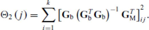
Note that j = 1, …, s.

If, on the other hand, it is known a priori that the inverse problem is inherently ill posed, it is possible to perform the compression at the beginning of the algorithm, precluding the diagnostic modification above. The following step can simply be included at the beginning of the basic algorithm:

Sequential OED algorithm: Modification 2 (Foreknowledge)

0. If the problem is inherently ill posed, determine G′_M by eq. (22) and update G_M←G′_M.

The main detriment to modifications 1 and 2 is the singular value decomposition. It is worth noting though that the SVD and associated ‘matrix compressions’ need to be evaluated only once. Once the compression is done, neither Θ₁(j) nor Θ₂(j) will evaluate to zero for all j because the zero singular values of G_M have been removed. This approach ‘frontloads’ the additional computational expense of the SVD and matrix compression. Nonetheless, if G_M is large, it may be infeasible to calculate its SVD. In that case, it may be possible to perform the compression through modified Gram-Schmidt orthogonalization. In fact, any truncated orthogonalization of G_M should suffice for the compression step.

Another way to get around the problem of determinant-based survey designs for ill-posed inverse problems is to design with respect to the regularized inverse problem. Constraints usually force the inverse problem to be well posed, which would free the designer from the SVD approach proposed here. Note that if data noise is independent and identically distributed (iid), the posterior model covariance matrix is C_m≡σ²_d (G^TG)⁻¹. Clearly, then Θ_D (eq. (5)) is directly proportional to the determinant of C_m. For regularized inverse problems, the model covariance matrix is

24

for iid data noise, where L is a generic regularization operator, and λ is parameter from 0 to 1 that governs the tradeoff between data rms error and the constraint imposed by L. It is thus natural to replace Θ_D with

25

The problem with this objective function - which is why it has not been adopted here - is that λ is a dynamic variable in the inversion, changing from iteration to iteration by the Levenberg-Marquardt algorithm. If λ were fixed, one could easily adapt the basic algorithm to accommodate Θ′_D, but different values of λ will mediate different survey designs. On the other hand, since this approach employs linearization, it effectively considers a single iteration of a non-linear inversion. It is therefore possible (and sometimes appropriate) to incorporate fixed λ in such cases, though we have not done so here. Haber et al. (2008) consider design methods for fixed λ.

2.3.2 MAR and experiment size

If the MAR is ζ, should the survey be deliberately designed to have exactly ζ design points, or is there added value in designing a larger survey?

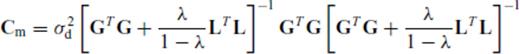
This is answered in part by considering the well-posed case, where ζ = . It is well known that the posterior model uncertainties decrease as data set size increases. The simplest form of posterior model covariance, mentioned in the last section, is C_m≡σ²_d(G^TG)⁻¹, where σ²_d is the variance of iid data noise. If each observation were repeated once, creating an augmented Jacobian G′ =[G^TG^T]^T, the posterior model covariance would become . The posterior model variances are halved by doubling the size of the experiment. There is clearly added value in this case to design surveys with more than ζ = observations. As discussed previously, an explicit relationship exists between the posterior model covariance matrix and the design objective function in eq. (5). Minimizing eq. (5) minimizes a global measure on the covariance matrix, so there is a direct connection between the design criterion, posterior model uncertainties and survey size.

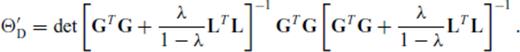
The situation is actually no different when the MAR is less than . If the inverse problem is inherently ill posed, model regularization is used to stabilize the inversion and to produce a unique solution. Taking as the posterior model covariance matrix the expression in eq. (25), if the experiment is again doubled, the posterior model covariance matrix is again approximately . The exact factor by which C_m is divided is more complicated (and depends on λ), but the gist of the argument is unchanged. Increasing the survey size beyond the MAR reduces posterior model uncertainty, and this is true irrespective of whether the MAR is less than or equal to the number of model parameters.

2.4 Borehole resistivity modelling and inversion

The synthetic example we have chosen to test our OED method on is a simple, single-borehole DC resistivity problem. Researchers have examined various aspects of axially symmetric borehole DC resistivity modelling and inversion for more than two decades (e.g. Yang & Ward 1984; Zemanian & Anderson 1987; Liu & Shen 1991; Zhang & Xiao 2001; Spitzer & Chouteau 2003; Wang 2003). These methods model the earth with a set of rectangular prisms that are treated as being axially symmetric about the borehole. Axial symmetry imposes a strong assumption on the lithological structure of the earth, for there are only a limited number of scenarios where this symmetry attains, particularly horizontal layering. Despite the strong restriction, axially symmetric geoelectrical imaging is useful in settings where data can only be collected from a single borehole, despite the limitation that the azimuthal position of a discrete three-dimensional anomaly cannot be pinpointed because of the non-directionality of source and receiver electrodes.

The borehole problem is cast in cylindrical coordinates (Fig. 1), and the forward and inverse problems are discretized using a transmission network analogy (Swift 1971; Madden 1972; Zhang et al. 1995; Shi 1998) adapted to cylindrical coordinates. The inversion is executed by non-linear least squares, using an L₁-norm regularization constraint on the gradient of the model parameters. Formally, the inversion objective function is

26

where d is the data vector, G is the Jacobian matrix and m is the model vector. The Levenberg-Marquardt algorithm (Levenberg 1944; Marquardt 1963) is used to regulate λ. Expanded details of the inversion can be found in the Appendix.

Figure 1.

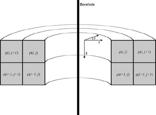
Cartoon of the borehole model. With a single borehole, resistivity is treated as being azimuthally invariant, reducing the problem from 3-D to 2.5-D.

Open in new tabDownload slide

2.5 Synthetic trials

The discretized model in Fig. 2 was used for testing the design method. The model depicts a 100-Ωm background with 20- and 500-Ωm embedded anomalies. The resistive anomaly has been deliberately placed partially in the ‘outer space’ region (Maurer & Friedel 2006) of the survey electrodes. It is widely recognized that the sensitivity of resistivity arrays drops off rapidly outside their ‘inner space’, the rectangular region adjacent to the array and bounded by the outermost electrodes. This is why, for example, dipole-dipole surveys produce geometric distortions of the inversion image at tomogram edges (Shi 1998). The model therefore simulates any situation where a survey has not, or cannot, incorporate anomalies in its inner space, or simply where no prior information was available to guide electrode placement. We have deliberately placed an anomaly straddling this ‘inner/outer space’ to establish whether the design method can provide any improvement there. To be clear, the purpose of the design criterion is to improve overall imaging accuracy through minimization of expected model uncertainties; it is not simply to improve image resolution in the ‘outer space’. The design technique might indeed improve resolution in this region, but this should be understood as a tangential benefit mediated by the true objective of the design criterion as just stated.

Figure 2.

Resistivity model. Ten electrodes (arrows) are placed at equispaced intervals of 1 m along the borehole, from the surface to a depth of 9 m. Background resistivity is 100 Ωm and anomalies A and B are 20 and 500 Ωm, respectively. The discretization is an irregular mesh, as suggested by the grid overlay, with cell size increasing as the distance from the survey. The mesh extends beyond what is shown here to accommodate boundary blocks needed for modelling accuracy (see Fig. 3). A total of 416 cells (model parameters) are used.

Open in new tabDownload slide

Ten borehole electrodes were simulated from the surface to a depth of 9 m at equispaced 1-m intervals. With 10 electrodes, eq. (15) indicates that there are 630 possible unique four-electrode observations. A 26 × 16 irregular mesh was used (including boundary condition cells), with cell sizes increasing proportionally as their distance from the borehole array (Fig. 3), so there are 416 model parameters in the inverse problem.

Figure 3.

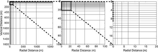
The 26 × 16 discretized mesh, at three different magnifications, that is used for forward and inverse modelling. The 10 borehole electrodes are shown in the right-hand panel.

Open in new tabDownload slide

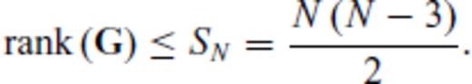
Eq. (16) tells us that the MAR for 10 electrodes used in four-electrode setups is 35. Since there are 416 model parameters, the un-regularized inverse problem is ill posed. The design algorithm thus employs modification 2 in Section 2.3.1, compressing the dimensions of G_M from 630 × 416 to 630 × 35. This eliminates zero singular values and ensures that the design algorithm will operate properly for experiments of more than ζ observations. This dimension reduction has the added advantage of making the design algorithm faster.

2.5.1 Random, standard and designed experiments with no prior information

Designed experiments are compared with randomly generated ones in a Monte Carlo simulation. Experiments were designed for a homogeneous earth model but deployed on the heterogeneous model in Fig. 2, which is one way of designing surveys when no prior geological information is available. Survey performances were evaluated for increasing numbers of observations, from 28 to 140. For each experiment size, 25 random experiments were generated and their data were synthesized and inverted. A dipole-dipole survey of 28 observations and the ERL survey (Earth Resources Lab, M.I.T.) with 140 observations were also compared as standard surveys (see Appendix for details).

2.5.2 Two-stage design with prior information

An approach to non-linear design problems is to create adaptive survey strategies that take advantage of linearized design. We propose an adaptive design strategy that executes in two stages. In stage one, a standard (or optimized) data set is collected and inverted to produce a reference model. The first stage can take advantage of prior information if any is available, but such information is neither needed nor assumed. In stage two, a survey is tailored to the reference model and a second data set is collected and inverted. The reference model serves as prior information in stage two.

The technique is demonstrated by taking as a reference the inversion result from a dipole-dipole data set of 28 observations (stage one). In stage two, experiments of 28 and 140 observations were designed with respect to the reference model and were compared with dipole-dipole and ERL surveys, both of which were also used as second-stage surveys. Additionally, a Monte Carlo study was conducted using 100 random 28-observation surveys, which were compared as second-stage surveys with a designed experiment of the same size.

2.5.3 Greedy design

The primary contribution this paper makes to geoscientific survey design is not a new objective function - as noted earlier, determinant-based design objective functions have been around a long while - but rather a greedy optimization approach for finding stationary points of this objective function. To demonstrate the computational savings of our design methodology and also to demonstrate the disadvantages of greedy optimization, we compare it with a genetic algorithm, which produces superior experiments (according to a determinant design criterion) but which takes longer to execute.

3 Results and Discussion

3.1 Random, standard and designed experiments

Fig. 4 shows Monte Carlo experiment performance curves comparing random, standard and designed experiments of different sizes. Three important features are apparent. First, designed experiments produce smaller model per cent rms errors than standard surveys. Second, designed experiments consistently produce smaller relative modelling errors than the p₅₀ for random experiments and are generally as small, or smaller, than the p₂₅ (meaning designed surveys are ∼75% likely to be superior to random surveys).

Figure 4.

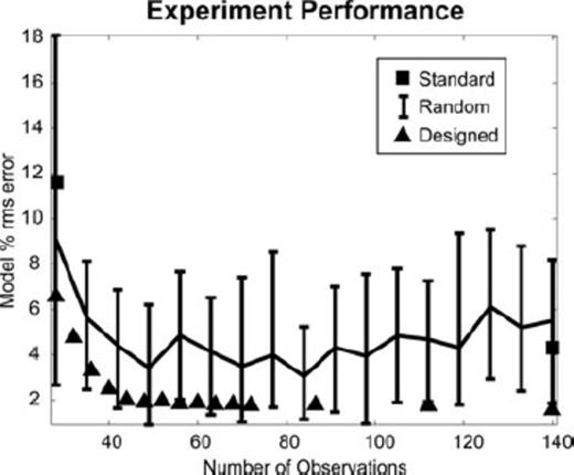
Experiment performances, measured by post-inversion model per cent rms error for the model in Fig. 2. Random, designed and standardized surveys are represented. The ‘random’ curve shows the approximate p₂₅, p₅₀ and p₇₅ for inversions done with 25 randomly generated surveys (25 for each experiment size). Survey designs were generated with respect to a homogeneous reference model but deployed on the model in Fig. 1. Data were noiseless.

Open in new tabDownload slide

Third, modelling errors asymptote for designed surveys after about 45 observations. This is probably associated with the MAR, which is 35 in this case. Modelling errors naturally decrease as experimental size increases, and the rate of decrease will be most rapid when experiments have fewer observations than the MAR, because each additional observation potentially reduces the solution null space by one dimension. However, the design performance curve does not asymptote exactly at 35 observations, which would be expected for noiseless data. This is probably because the conditioning of the Jacobian is initially poor at 35 observations, even though it has reached the MAR. Additional observations beyond this will further increase the determinant of G^TG, thereby improving the conditioning and quickly causing errors to asymptote.

While designed surveys produce smaller model per cent rms errors than most random surveys, they are evidently not superior to all such surveys. It is important to remember that the sequential OED algorithm is crafted to be expeditious, and it consequently produces experiments that are not necessarily globally optimal. This means that there is some probability that randomly generated experiments can outperform ones designed by this method. Still, the odds are in favour of the design methodology, as is clear in Fig. 4, and it is worth stressing that the designed surveys outperform both standard experiments in this demonstration. At the end of the day, globality can only be guaranteed by global search algorithms, but their computational complexity is high. We revisit this tradeoff in Section 3.3.

Another important point to keep in mind is that the surveys designed in this exercise were optimized with respect to a homogeneous earth, not the heterogeneous model in Fig. 2 on which they were deployed. It is a revelation that geoelectrical experiments designed for a homogeneous half space can produce such superior results for a heterogeneous earth. This is an indication of how much room for improvement there is in geoelectrical data acquisition.

3.2 Two-stage design with prior information

The preceding surveys were designed without prior information, but the design technique can easily be set up for adaptive experimental design, where surveys are adapted according to (prior) information that becomes available over time.

Fig. 5 shows results for two-stage design technique. With prior information this adaptive strategy performs well. The 28-observation design (panel a) reduced model per cent rms errors by over an order of magnitude compared to the initial survey. Importantly, the designed survey captured the correct shape of the 500-Ωm resistive anomaly, which was misrepresented in the original image. Compared with the 28-observation examples in Fig. 4, this small, adapted experiment performs exceptionally. Panel (b) shows the result for a 140-observation designed experiment. The model per cent rms error for this designed experiment is better than the result in panel (a) but only marginally, suggesting that the smaller experiment would practically suffice in view of financial considerations. Both designed experiments outperform the ERL survey shown at right in panel (b).

Figure 5.

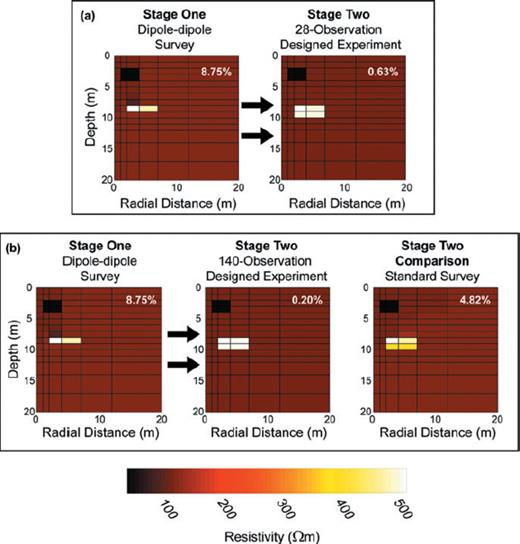
Results of two two-stage, adaptive designs. Post-inversion model per cent rms errors are shown in the top right corner of all panels. Data were noiseless. The stage-one survey in both examples is the 28-observation dipole-dipole survey (left-hand panels). (a) Results for a 28/28 design (28 observations for the dipole-dipole survey, 28 for the designed experiment). (b) Results for a 28/140 design (middle panel) and those for a 28/140 ‘standard’ survey (right-hand panel; stage one: 28-observation dipole-dipole survey; stage two: 140-observation ERL survey).

Open in new tabDownload slide

These results are encouraging: small, adapted experiments, using our sequential design methodology, can significantly improve data quality without resorting to computationally expensive non-linear design techniques. In panel (a), only 56 observations were made (28 for the dipole-dipole and 28 for the designed survey). By comparison, the ERL survey used 140 observations without producing a better image. The conclusion is plain: rather than collect a large data set, which might present a significant financial obstacle, this simple two-stage technique can be employed to produce superior imaging capabilities at a fraction of the cost.

To determine whether the 28-observation design produced a statistically significant improvement in the acquisition strategy, it was compared with 100 random experiments of 28 observations employed as second stage surveys. The histogram in Fig. 6 shows the result; the experiment designed with prior information from the reference model outperformed more than 95% of random surveys, showing that the technique produces experiments whose information content is statistically significantly superior.

Figure 6.

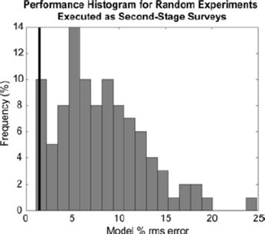
Histogram showing the frequency distribution of model per cent rms errors for random experiments of 28 observations executed as second-stage surveys, compared with an adapted experiment also executed as a second-stage survey (black line). The data were noiseless. The input model for all inversions was the stage-one dipole-dipole inversion in Fig. 5. The black line at left shows the model per cent rms error attained for the adaptively designed experiment of 28 observations. The model per cent rms error of the designed experiment is in the lowest 5th percentile, meaning it outperformed 95% of the random experiments.

Open in new tabDownload slide

3.3 Greedy design

Fig. 7 shows the CPU time for experimental designs of increasing numbers of observations. All computations were carried out on an HP laptop with dual 2 GHz processors and 2 GB RAM. The key point is that the sequential OED methodology executes in a matter of seconds. This is in contrast to traditional global search methods that must evaluate the objective function in eq. (5) thousands or millions of times. Importantly, global search methods must explicitly evaluate eq. (5) for each trial experiment, without the benefit of numeric tricks like the update formulae in Section 2.1. Consequently, global search methods require orders of magnitude more CPU time than are needed for our fast, sequential design algorithm.

Figure 7.

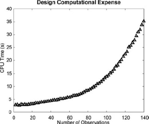
Computational expense for the sequential design algorithm.

Open in new tabDownload slide

The demonstration problem in this paper is small - there are only 630 possible observations and 416 model parameters, making G_M manageably small. Larger 2.5 D geoelectrical problems can easily have tens of thousands of permitted observations and thousands of model parameters. However, this should pose little problem for this design procedure because it relies on update formulae, an approach also adopted in part by Wilkinson et al. (2006b). Explicit evaluation of a determinant or matrix inverse is an O(n³) operation, but these are replaced by matrix-vector multiplications, which are O(n²) operations. The computational complexity is therefore probably comparable to the sequential design procedures outlined by others (Curtis et al. 2004; Stummer et al. 2004), though it is claimed that Stummer et al.'s procedure is actually O(n) (Wilkinson et al. 2006b). Moreover, that resistivity data sets are generally information-limited, as discussed in Section 2.2, means that the master Jacobian, G_M, can be usefully compressed to have only columns, as per eq. (16). As noted elsewhere, this operation needs to be performed only once, the consequence of which is that the dimensions of G_M can be losslessly reduced, making the design algorithm faster to execute. In this paper, we have used the truncated SVD to effect this compression but recognize that the SVD itself may be intractable for large problems. We have suggested that the compression operation can equally be effected through use of the modified Gram-Schmidt method or any other technique that rapidly finds an orthonormal basis spanning the range of G_M.

Fig. 8 compares the CPU time of our sequential design method with that for a genetic algorithm (a global search algorithm) maximizing the same design objective function. The same earth model in Fig. 2 was used in both design cases. The objective value () of each survey design is plotted against the number of observations.

Figure 8.

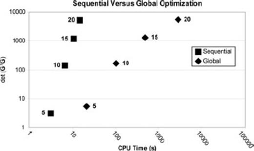
Sequential design versus global optimization. The design objective function, , is plotted against CPU time for designs produced by the sequential design algorithm (squares) and a genetic algorithm (diamonds). Numbers next to the ‘Sequential’ and ‘Global’ icons indicate the number of observations for which the experiments had been designed.

Open in new tabDownload slide

The conclusions to be drawn from Fig. 8 are clear. First, the slope of the sequential design curve is steeper than the slope for the global design curve. This means that the quality of sequentially designed surveys increases more rapidly per unit of computation time than that for globally designed surveys. Second, the disparity between the quality of sequentially and globally designed surveys decreases as the number of observations increase. In effect, the larger the experiment, the closer to global optimality comes the sequential design algorithm. Hence, the sequential design produces suboptimal surveys that approach optimality as the size of the experiment increases and at rate significantly faster than global optimization strategies.

4 Conclusion

A novel algorithm for linear(ized) sequential experimental design was developed and demonstrated. The design objective function was , which is common to design theory. This objective function is known to be a proxy for global model uncertainty, the maximization of which is a common experimental design objective. Determinant-based design objective functions are computationally expensive to evaluate, making them impractical for real-world application. Critically, we introduced update formulae that minimize this computational expense in a greedy, sequential algorithmic framework.

Several demonstrative examples were provided, showing the utility of the design technique for a simple 2.5-D borehole example. The first of these was a design problem with no prior information wherein experiments were designed with respect to a homogeneous earth model but deployed on a heterogeneous target. Designed experiments in this investigation were shown to be statistically superior to random or standard surveys deployed on the same target.

A novel, adaptive experimental design procedure was also introduced that avails itself of prior information and which proceeds by using computationally efficient linearized design theory. Results demonstrated that this adaptive sequential design method can be usefully applied in situations where incomplete or inaccurate prior information is available. Inversions using adaptively designed surveys produced statistically significant improvements in model errors as compared with random and standard surveys, suggesting that the approach can serve as an effective alternative to computationally expensive non-linear design techniques.

Of primary significance is the development of a greedy algorithm methodology that designs surveys by sequential, local optimization of the determinant-based objective function. This methodology is further enhanced by update formulae that reduce computational complexity from O(n³) to O(n²). In contrast, it was shown that a comparable global search algorithm takes orders of magnitude more time to produce an OED. On this fact alone, it is easy to appreciate that this design technique can realize substantial time savings compared with global methods.

Lastly, it was seen that the quality of sequentially designed experiments approaches global optimality as the size of the experiment increases. Thus, the new algorithm not only requires a fraction of the computation time but it also approaches global optimality as the size of the experiment increases.

References

Appendices

Appendix A: Dipole-Dipole Survey

The dipole-dipole survey is tabulated below. A and B designate the positive and negative transmitter electrodes, respectively; M and N designate the positive and negative receiver electrodes, respectively.

Open in new tabDownload slide

Appendix B: Erl Survey

Open in new tabDownload slide

Appendix C: Proofs For Updates To

Given a block matrix , where , B∈^p×n and m+p ≤ n, the determinant of A′ A′^T is given by

(C1)

Proof: The auto-outer product of A′ is

(C2)

Transform (C2) by the following right multiplication:

(C3)

Taking determinant produces

(C4)

and taking advantage of the fact that the determinant of a block upper (or lower) triangular matrix is the product of the determinants of its diagonal blocks (Golub & Van Loan 1996), the second and third determinants in eq. (C4) reduce to

(C5)

Substituting (C5) into (C4) completes the proof.

Dividing (C1) by and substituting the vector a^T for the matrix B, we have

(C6)

Because I−A^T (AA^T)⁻¹A is idempotent, Θ₁ can also be expressed as

(C7)

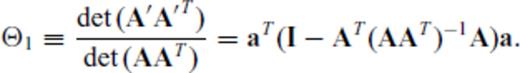
Tangentially, eqs (C6) and (C7) express the squared norm of the projection of a onto the row null space of A (because A^T (AA^T)⁻¹A is the projection matrix of A).

Appendix D: Proofs For Updates To

Given a block matrix , where , and m+p > n, we can find the determinant of A′^TA′ by starting with the expression

(D1)

which expands to

(D2)

By virtue of the identity

(D3)

it follows that

(D4)

hence,

(D5)

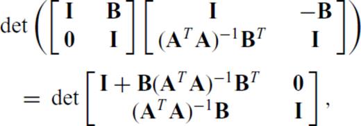
Defining B = a^T yields

(D6)

Note that

(D7)

so

(D8)

Dividing by yields

(D9)

This last expression is well-known in design theory and is used for designing so-called D-optimal experiments (e.g. Atkinson et al. 2007). It was independently published by Fedorov (1972) and Wynn (1970).

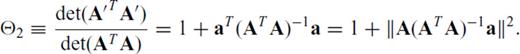
Appendix E: Proofs for Updates to (AA^T)⁻¹

Proofs of the SMF for updates to (A^TA)⁻¹ can easily found in any good reference. However, updates to (AA^T)⁻¹ are not so straightforward, as the dimensions of AA^T change if one or more rows are appended to A.

Given a block matrix , where , and m+p > n, it is straightforward to algebraically derive the inverse of A′ A′^T, which is

(E1)

where

(E2)

Defining B = a^T, eq. (E1) simplifies to

(E3)

where

(E4)

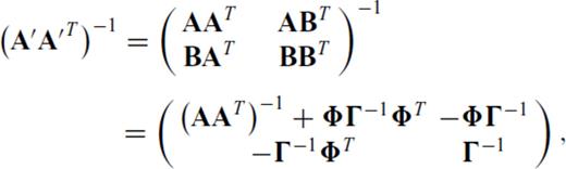
Appendix F: Forward and Inverse Modelling

The model was discretized into an irregular mesh with cell size increasing as a function of distance from the borehole electrodes (Fig. 3). Resistivities were treated as azimuthally invariant, per Fig. 1. The large, distant blocks are needed to help accurately predict electrical potentials and electrode sensitivities near the borehole. Modelling was done through an adaptation of the transmission network analogy for cylindrical coordinates.

The inversion was done by non-linear least squares and is described below. The objective function combines data rmse and L₁ smoothness regularization:

(F1)

where d is the data vector, G is the Jacobian, m is the model parameter vector, ∇m is the spatial gradient of the model, λ is the tradeoff parameter between data rmse and the model smoothness constraint. The tradeoff parameter varies dynamically from iteration to iteration and is controlled by the Levenberg-Marquardt algorithm.

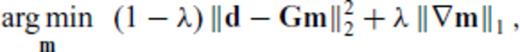
Consider the 1-norm of ∇m in eq. (F1); this is called total variation regularization in inverse theory and is inspired by methods of image reconstruction and denoising from digital imaging theory (Rudin et al. 1992). It has the nice property that it permits sharp boundaries in the solution of inverse problems (Rudin et al. 1992), which is why it has been adopted in this work.

In addition, the inversion has been further stabilized by bounding resistivity values to between 0 and 10⁴Ωm. This was effected through the simple parameter substitution,

(F2)

where m_i is the resistivity of the ith cell and is the substitute variable for which the inversion formally solves. The chain rule is used to express the partials of the forward operator, call it g, with respect to γ. If and then

(F3)

Non-linear updates in the inversion code therefore take the form

(F4)

where Δd is the residual between observed and predicted data.

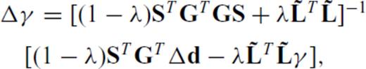
The matrix relates to the L₁ norm of ∇m and depends on a modification to the ordinary first difference matrix, L. The 1-norm of the gradient of m is approximated by

(F5)

using Einstein notation. Following the ideas of Scales & Gersztenkorn (1988), the partials of (F5) with respect to m are given by

(F6)

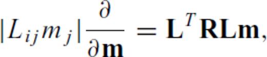
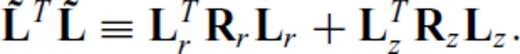
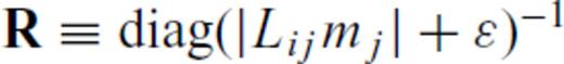where and ɛ is a small pre-whitening term to prevent blow-up if any element of L_ijm_j is zero. Letting L_r and L_z denote the ordinary 1st-difference operators in the radial and depth directions, respectively, we therefore define the partials of ∥∇m∥₁ as

(F7)

and hence

(F8)