Transient electromagnetic response of a loop source over a rough geological medium Free

Summary

Introduction

The central goal of electromagnetic (EM) induction geophysical studies of the non-magnetic and non-polarizable Earth is to infer the subsurface electrical conductivity distribution based on terrestrial, marine, airborne, downhole or satellite measurements of electromagetic fields that develop in response to transient excitation of the subsurface by an internal or external, natural or artificial, source or array of sources. Electrical conductivity σ(r) appears along with the magnetic permeability of free space μ₀ as the product μ₀σ(r) in the governing pre-Maxwell diffusion equation. Traditionally, the geological medium is characterized by a piecewise smooth spatial distribution of electrical conductivity. However, such a description cannot always be justified if it is accepted that most physical properties, including electrical conductivity, of geological media are often spatially rough across many decades of length scale (e.g. Pilkington & Todoeschuck 1993; Painter 1996; Tennekoon et al. 2005; Molz & Hyden 2006). It has recently been shown (Weiss & Everett 2007) that a fractional diffusion equation can provide the basis for a simple and straightforward extension of classical EM induction, which naturally takes into account the inherent roughness of geological media. We define a rough physical property as one which exhibits persistent spatial correlations over a wide range of length scales so that it possesses a power-law wavenumber spectrum (Everett & Weiss 2002).

In this paper, the transient EM response is computed for a horizontal loop source, excited by a step-off current, that is located on a rough half-space in which the electrical conductivity is characterized by a spatially uniform roughness parameter β, with 0 < β < 1. The solution to the rough geology problem explored in this paper generalizes classical solutions (corresponding to the limit β → 0) for the EM response of a loop over a uniform conducting half-space. The classical problem has been analysed by many workers including Wait (1951), Morrison et al. (1969) and Ryu et al. (1970). Additional details are found in Ward & Hohmann (1987). In the rough case, we formulate and then readily solve a governing fractional differential equation in the Laplace s-domain. The conversion of the Laplace-domain solutions into the time domain is performed using the Gaver-Stehfest (GS) algorithm (Gaver 1966; Stehfest 1970), which has previously been used in EM geophysics by Knight & Raiche (1982) and Everett & Edwards (1993), amongst others.

Frequency Domain Analysis

The analysis of the fields caused by a transient loop lying on a homogeneous rough medium starts from the conventional Ampere's law ∇ × B = μ₀J but with the added feature that it incorporates a generalized time-convolutional form of Ohm's law J = σ_β*E, so that

1

In eq. (1), σ_β is a generalized electrical conductivity. The time convolution operator and generalized conductivity in eq. (1) are defined below. The displacement current density J_D = ε₀∂E/∂t that normally appears in eq. (1) is safely neglected in EM induction studies. Equivalently, the characteristic angular frequency ω is sufficiently low so that σ ≫ ωε₀. In eq. (1), J_S(t) describes the horizontal loop source current density,

2

The axisymmetric loop, of radius a, is centred about the origin of a cylindrical coordinate system (ρ, φ, z) in which the vertical coordinate z is positive downward, so that Earth occupies the lower half-space z ≥ 0. Thus, the centre of the loop is located at ρ = 0. The delta function δ(t) indicates an impulse of strength I in the loop current that occurs at time t = 0. Later, we will consider step-on and step-off current excitations. The other relevant Maxwell equation is Faraday's law

3

The magnetic field B can be eliminated from eqs (1) and (3), leading to a convolutional vector diffusion equation for the electric field E, namely

4

As shown previously (Weiss & Everett 2007), the convolutional diffusion equation for the electric field E can be cast as a fractional diffusion equation. This is achieved here via the introduction of a generalized Ohm's law according to the convolution

5

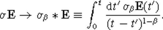
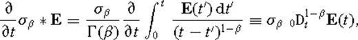
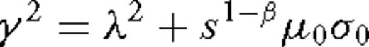
The generalized conductivity σ_β has dimensions of , where the usual dimensions of conductivity σ in SI units are [σ]= A V⁻¹ m⁻¹ = A² s³ kg⁻¹ m⁻³. Accordingly, we can write σ_β∼στ^−β, where τ is a parameter with dimensions of time, [τ]= s. Note that this form for the generalized electrical conductivity σ_β is appropriate for the anomalous diffusion coefficient of a spatially rough medium (Metzler & Klafter 2000). In fact, the quantity σ_β is referred to as the ‘anomalous electrical conductivity’ in Weiss & Everett (2007). The consequence of using the generalized Ohm's law (5) is that EM induction becomes an anomalous diffusion process in a geologically rough medium.

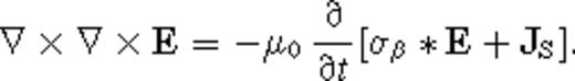
A generalized Ohm's law J = σ*E has been used in geophysics to model EM induction in a polarizable medium (e.g. Smith et al. 1988). Typically, modelling EM induction in such a medium is performed in the frequency domain, in which case Ohm's law becomes the product J(ω) = σ(ω) E(ω), and the governing Maxwell equations are solved for a given frequency assuming a time-harmonic source excitation. Here we employ a time-domain convolutional Ohm's law for the entirely different purpose of describing transient EM induction in a non-polarizable, but spatially rough medium.

The time derivative of eq. (5), which is required to solve the governing eq. (4), is

6

where we have introduced the fractional derivative or Riemann-Louiville operator (Metzler & Klafter 2000, their eq. 35)

7

and Γ is the Gamma function which serves simply as a normalizing constant. See Oldham & Spanier (1974) for a discussion on the origin and role of the Gamma function in the development of fractional derivatives. Inserting eq. (7) into the convolutional vector diffusion eq. (4) yields

8

which is the sought-after vector fractional differential equation for the electric field E(r, t) governing EM induction in a spatially rough medium. Note that, in the special case of a smooth medium in which the roughness parameter β → 0, the fractional diffusion eq. (8) reduces to the classical diffusion equation ∇ × ∇ × E = −μ₀∂/∂t[σE + J_S], as it should.

The fractional diffusion eq. (8) is conveniently solved in the Laplace s–domain since the Laplace L{ } of a fractional derivative of a function f(t) is analytic (Metzler & Klafter 2000), namely

9

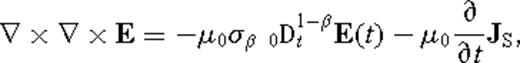
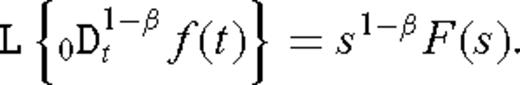
Note that the Laplace transform in eq. (9) reduces to the familiar formula in the case β → 0. It is assumed throughout that f(t) → 0 as t → 0₊, that is, the function f(t) vanishes as time t approaches zero backwards through positive values. This assumption is valid since we are Laplace transforming the impulse response. Taking a Laplace transform of the fractional vector diffusion eq. (8) yields

10

where e (s) is the Laplace-transformed electric field E(t) and j_S(s) is the Laplace-transformed source current density J_S(t). It is clear that the rough-geology problem is identical to the classical problem (Morrison et al. 1969; Ryu et al. 1970) except that, in the first term on the right-hand side of eq. (10), we have s^1−β instead of s.

The solution to eq. (10) can now proceed along standard lines. Since the loop source is axisymmetric and horizontal and lies atop a half-space defined by a plane of constant z, symmetry dictates that the electric field is azimuthally directed with no functional dependence on azimuth φ:

11

Inserting eq. (11) into eq. (10), taking a Hankel transform and enforcing the fundamental EM boundary conditions at the interface z = 0 leads, after some algebra, to the solution in the overlying air half-space as

12

where

13

and the reflection coefficient R is

14

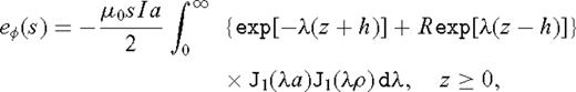
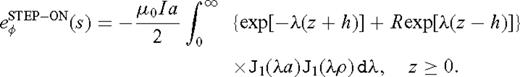
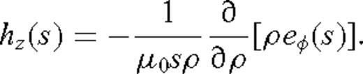
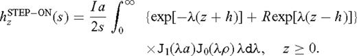
The function appearing in eq. (12) is a first-order Bessel function, whereas h is the loop height above the ground surface z = 0. As mentioned earlier, we are interested in the transient step-off response since that quantity is recorded by many commercial time-domain EM systems. It is convenient to first compute the step-on response, which in the Laplace domain, is found using the formula

15

where u(t) is the Heaviside step-on function defined by

16

The step-on response in the Laplace domain is therefore e_φ(s)/s, or

17

The azimuthal electric field component e_φ(s), at least in the underlying half-space, is interesting from a theoretical perspective since it is proportional to the eddy current density. However, e_φ(s) is not directly related to a practical field measurement. The vertical magnetic field h_z(s), on the other hand, is proportional to the actual voltage that develops in the loop, as measured by most commercial sensors. In the Laplace domain, h_z(s) is readily found from Faraday's law (eq. 3) as

18

Using eq. (18) along with the Bessel function identity

19

the step-on vertical magnetic field becomes

20

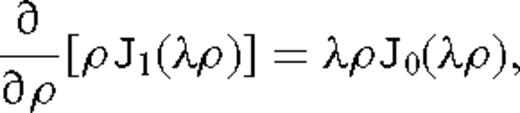
The function appearing in eq. (20) is a zeroth-order Bessel function. For convenience and without sacrificing physical insight into the behaviour of the transient EM response, we assume that both the transmitter and the receiver are located on the surface of the rough half-space. Setting h = 0 and z = 0 in eq. (20) results in

21

The commercial time domain EM systems generally measure the response to a rapid linear ramp-off in transmitter current. To a good approximation, unless otherwise noted, the ramp-off time is sufficiently short so that the ramp-off response is equivalent to the step-off response. Accordingly, we use the Heaviside step-off function is 1 −u(t) and compute the step-off response as the difference between the late-time, or DC, response and the step-on response:

22

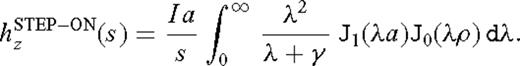
Time Domain Analysis

Although a multitude of approaches for inverting the Laplace transform (Davies & Martin 1979; Hüpper & Pollak 1999) are available, the popular GS method (Gaver 1966; Stehfest 1970) has long proven reliable for computing transient controlled-source EM responses in geophysics (Knight & Raiche 1982; Edwards & Cheesman 1987; Everett & Edwards 1993; Das 1995).

Suppose a function g(s) is available in the Laplace domain, and the corresponding function G(t) is required in the time domain. The GS approximation to G(t) is defined by

23

where the GS coefficients {c_j(n)} for j = 1, 2, …, n, with n even, are

24

A detailed derivation of the GS algorithm is given in Everett (1990). We find that the linear combination of terms appearing in eq. (23) provides accurate results for n in the range 12–18, when programmed in standard 64-bit arithmetic. The optimal number of GS coefficients, for a given set of model parameters, has to be determined by numerical experiment. Larger values of n (>18) lead to excessive rounding errors as successive terms in the series alternate in sign and can grow large in magnitude. The use of smaller values of n(<12) provides less accuracy. In general, the GS algorithm is stable for transient functions G(t) such as EM responses, which exhibit no discontinuities, sharp peaks or rapid oscillations. Note that, according to eq. (23), the Laplace domain function g(s) needs to be known only at the n real values of s given by s_j = j ln 2/t where j = 1,2,…, n. Thus, the GS algorithm does not require complex variables which simplifies the computer programming. For reference, the GS coefficients for n = 8– 18 are given in Table 1.

Table 1.

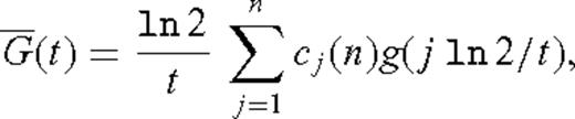
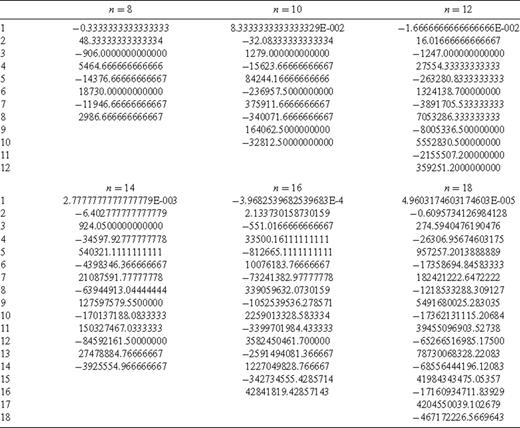
Gaver-Stehfest coefficients for n = 8 through 18.

Open in new tabDownload slide

Results

The essential goals of this paper are threefold: (1) to develop the mathematical formulae for the transient loop response of a rough geological half-space; (2) to present some EM response curves as a starting point for developing a better understanding of the physics that is introduced by associating a roughness parameter β to the geological medium; (3) to expose the practitioner to the range of transient EM response waveforms that might be found in actual field measurements. The papers by Everett & Weiss (2002) and Weiss & Everett (2007) provide field evidence that certain EM loop responses appear to be consistent with an underlying, spatially homogeneous rough medium. Additional field studies are, of course, necessary and encouraged, but beyond the scope of this paper.

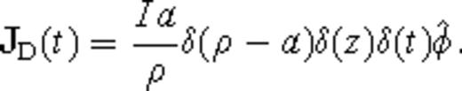
In view of the foregoing remarks, in Fig. 1 are shown step-off transient EM responses for a canonical set of typical but otherwise arbitrary model parameters: a loop of radius a = 1.0 m and current I = 1.0 A situated at height h = 0.1 m above a ground of uniform conductivity, σ = 0.1 S m⁻¹. The nominal distance from the transmitter (TX) to the receiver (RX) is L = 100 m. The responses shown in the figure are generated by using the GS algorithm to invert the step-off Laplace-domain EM response given in eq. (22), which is proportional to the measured RX signal. The roughness parameter β is varied between β = 0.0 (the classical case) and β = 0.5, as shown in each of the panels. The solid line in the top left-hand panel making a 68.2° dip angle to the horizontal axis of the log-log plot of transient RX voltage marks the slope of the late-time asymptotic response. The slope has the familiar γ = −5/2 value (Ward & Hohmann 1987) that is associated with the t^−5/2 late-time power-law decay of classical EM signals diffusing into a uniform half-space. The γ = −5/2 value is well known to be independent of the loop radius, current and height as well as the conductivity of the ground and the TX-RX separation distance. The other panels in the figure show equivalent step-off responses computed for increasingly larger values of the roughness parameter β, with the classical response (light grey lines) shown for comparison. A systematic decrease in the slope γ magnitude of the late-time response is apparent, from γ = −5/2 for the classical case to γ = −3/2 for the β = 1/2 case. The differences in the responses are certainly large enough to be detected in field data. The value of the late-time slope is thus readily measurable and could be used by practitioners as diagnostic of an apparent roughness of the ground. A simple analytic relationship between γ and β has not been found although, as shown in Fig. 2, the formula γ∼β− 2 roughly holds for β > 1/4.

Figure 1.

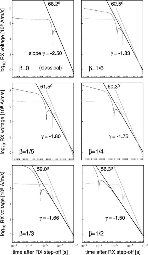
Step-off transient RX voltage as a function of roughness parameter β. The classical response (top left-hand panel) is shown in grey in the other panels for comparison with the situations when β > 0. The dotted curve in each panel represents a negative transient.

Open in new tabDownload slide

Figure 2.

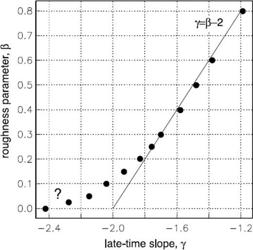
Relationship between late-time slope γ and roughness parameter β based on Gaver-Stehfest computations. The question mark as β approaches zero is explained in the text.

Open in new tabDownload slide

The accuracy of the GS algorithm is not sufficient to compute the response to ‘very late’ times well beyond t = 0.1 s. Dr Tilman Hanstein (private communication, 2008) has used a fast Hankel transform method to extend the response calculations out to three decades later in time. He has found that the relation γ = β− 2 may actually extend to lower values of β than is indicated by the GS results shown in Fig. 2, with possibly an irregularity at β = 0. Confirmation of the low-β, ‘very-late’ time behaviour is beyond the reach of the GS algorithm and the scope of this paper. For this reason, a ‘question mark’ has been added to Fig. 2. Nevertheless, the behaviour of the ‘very late’ slope when the roughness parameter β approaches zero has no practical relevance because the effects found by Dr Hanstein are only visible in a time range, which is far beyond the times for transient electromagnetics (TEM) land systems with the separate loop configurations. For all practical purposes in which conventional TEM land systems are used, the results in Fig. 2 shall provide a reliable indication of the late-time slope that would be observed in the field at low β values.

While the t^−5/2 classical power-law decay does not depend on the ground electrical conductivity σ or TX-RX separation distance L, it is of interest to inquire whether EM late-time transients from a rough geological medium are similarly robust with respect to these model parameters. Shown in Fig. 3 is the step-off response with roughness parameter β = 1/3 for the canonical model, except that electrical conductivity σ is varied from 0.1 to 0.3 to 1.0 S m⁻¹. The TX-RX separation distance L is similarly varied from 50 to 100 to 200 m in Fig. 4, all other model parameters retaining their nominal values. It is readily seen that the late-time asymptotic slope of the step-off response, in this case γ = −5/3, remains invariant with respect to adjustments in the parameters σ and L. These results suggest that the power-law slope γ = −5/3 is a characteristic late-time feature of EM signals diffusing into a geological half-space described by roughness parameter β = 1/3.

Figure 3.

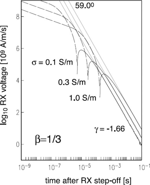
Step-off transient RX voltage as a function of electrical conductivity σ, for roughness parameter β = 1/3.

Open in new tabDownload slide

Figure 4.

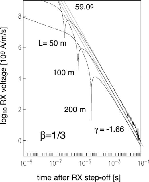
Step-off transient RX voltage as a function of TX-RX separation distance L, for roughness parameter β = 1/3.

Open in new tabDownload slide

An important feature of step-off EM transient responses is the zero-crossing time τ_H, which measures the time after step-off that it takes for the induced voltage in the RX loop to change sign. The sign reversal may be viewed conceptually as the passage of the subsurface eddy current ‘smoke ring’ vortex beneath the RX loop (Nabighian 1979). A field measurement of the zero-crossing time is diagnostic of the subsurface electrical conductivity and, in fact, is sometimes used to define an apparent ground conductivity. The zero-crossing is easily recognized; it occurs at the time at which the cusp appears in the log-log plots of the transient step-off responses. Weiss & Everett (2007) present a theoretical argument, based on the treatment of EM induction in a rough geological medium as a continuous time random walk (Metzler & Klafter 2000), which suggests that the zero-crossing time τ_H should scale with the TX-RX separation distance L according to τ_H∼L^2/(1−β) (Note that the α parameter used in Weiss & Everett 2007, is related to the β parameter used in this paper by ). We can check their scaling relation by computing step-off EM transients and plotting the zero-crossing time as a function of TX-RX separation, for a number of different roughness values. This has been done and the result appears in Fig. 5. The computed zero-crossing curves τ_H(L) have been plotted on a log-log scale for roughness parameters varying from β = 0 to 1/2. A power-law relationship between τ_H and L is confirmed by the straight line nature of the plots. In the general case, to a remarkable precision, we note that the slope m is related to the roughness parameter β by the formula m = 2/(1 −β). This result confirms the power-law relation τ_H∼L^2/(1−β) that was suggested by Weiss & Everett (2007) and lends strong support to the concept that EM induction in a rough geological medium is equivalent to a continuous time random walk undertaken by the current elements of the eddy current vortex. Shown in the inset to Fig. 5 are the τ_H(L) data from the Brazos (TX) floodplain, which have been earlier analysed by Weiss & Everett (2007). The data are fit remarkably well using a roughness parameter β = 0.12 with conductivity σ = 0.6 S m⁻¹. Fitting the remarkably linear τ_H(L) curve using a traditional layered or smooth conductivity model σ(z) requires a large number of model parameters.

Figure 5.

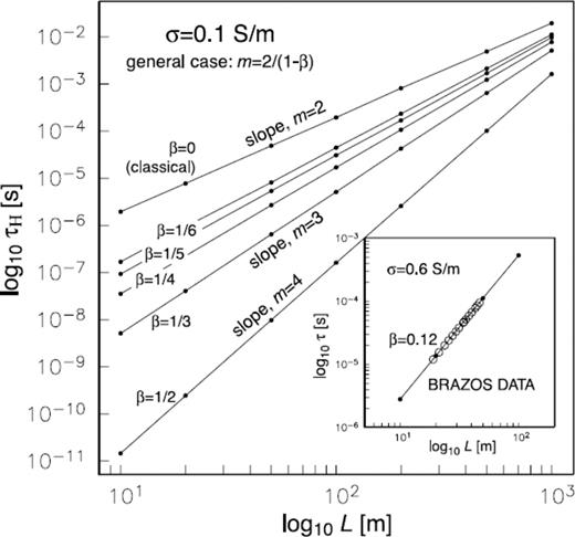
Log-log plot of RX voltage zero-crossing time τ_H(L) as a function of roughness parameter β. The Brazos County data, which fit the anomalous diffusion concept, are shown in the insert.

Open in new tabDownload slide

The results obtained so far in this paper have indicated that the slope of the late-time step-off transient EM response over a uniform conducting half-space is indicative of the roughness parameter β. Departures from the classical γ = −5/2 value vary systematically with roughness parameter β. However, in practical EM systems, especially as the loop size gets larger, it is difficult to transmit a perfect step off. Unwanted transient oscillations similar to a Gibbs phenomenon occur in a TX loop current I(t) that is abruptly switched off. For this reason, manufacturers will design a linear ramp-off function that takes the TX current from its steady value I₀ down to zero over a short period of time, typically measured in μs and known as the ramp-off time τ_R. Since practical instruments will record the ramp-off response, it is of interest to this study to examine the effect of a typical ramp-off time τ_R on the late-time slope γ of the classical EM transient response. In this way, we can determine whether there is any ambiguity between geological roughness β and ramp-off time τ_R in so far as possible departures from the classical value γ = −5/2 of the late-time slope may be concerned. The classical ramp-off response is readily computed by convolving the linear ramp function with the classical impulse response, a standard calculation (Fitterman & Anderson 1987). The result is shown in Fig. 6 for ramp-off times varying from 0 to 100 to 500 μs. It is readily observed from the figure that the ramp-off time τ_R has only a very small effect on the slope of the late-time response. The angle of the late-time response slope with the log-log horizontal axis changes from 68.2° for the classical case to 69.0° for the τ_R = 500 μs case. The associated change in γ is much smaller than the changes in γ that were seen in Fig. 1 as the roughness parameter β was varied. Furthermore, the slope γ magnitude increases as the ramp-off time increases from zero, whereas ǀγǀ in Fig. 1 decreases as the geological roughness increases from zero. Thus, it seems clear that practitioners would not mistake any subtle shift in the late-time slope associated with a finite ramp-off time with the much larger, and opposite-polarity, shift in γ that is caused by geological roughness.

Figure 6.

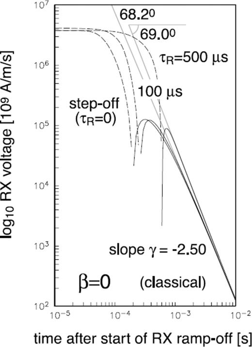
Ramp-off transient RX voltage as a function of ramp-off time τ_R.

Open in new tabDownload slide

As a final illustration of the practical interpretation of EM transient responses acquired over a geologically rough terrain, it is of interest to inquire whether an observed departure from the classical γ = −5/2 value of the late time slope may also be caused by layering of the electrical conductivity structure. Indeed, in Fig. 7 we show computed step-off classical responses for two-layer earth models, alongside the response of the canonical half-space model. The responses of a resistor-over-conductor (r/c) and a conductor-over-resistor (c/r) are shown. Note that, indeed, the late-time slopes of the two-layer model responses depart significantly from the γ = −5/2 value exhibited by the response of the canonical half-space model. It therefore appears that a field measurement of the late-time slope of the transient response cannot be used to distinguish between layering and apparent roughness. However, as shown in Fig. 8, the zero-crossing curve τ_H(L) provides vital information, which can resolve ambiguities. The τ_H(L) curves for the two-layer models are non-linear, in contrast to the linear moveout of the classical half-space model. Indeed, a linear τ_H(L) moveout curve is generated for any value of roughness β, as we earlier have shown in Fig. 5. Specifically, the r/c model zero-crossing curve contains a kink at L∼ 40 m, whose origin is due to the presence of the subsurface conductivity contrast at h∼L/2 = 20 m. The c/r model zero-crossing curve flattens out with increasing L due to the underlying resistive layer, which, as is well-known, tends to shorten the zero-crossing time at large TX-RX separations. To summarize, both layering and geological roughness generate departures from the classical late-time slope value of γ = −5/2. However, an apparent roughness generates a linear τ_H(L) moveout curve, unlike the layered models. Thus, a rough geological model can be distinguished by a practitioner from a classical layered model by examining in field responses both the late-time slope and the shape of the zero-crossing moveout curve. Although it is conceivable that a multilayered model could generate a power-law τ_H(L) moveout curve, such a model would require several or more model parameters to describe. A spatially uniform rough geological model would require only the specification of a single parameter β to explain the same power-law moveout behaviour.

Figure 7.

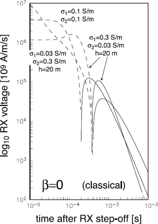
Step-off transient RX voltage for 2-layer conductivity models.

Open in new tabDownload slide

Figure 8.

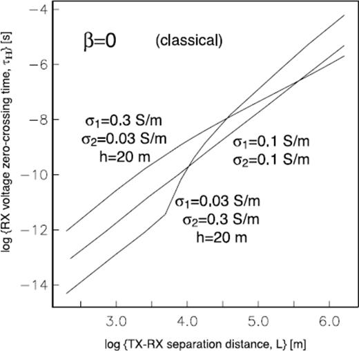
Log-log plot of RX voltage zero-crossing time τ_H(L) for two-layer conductivity models.

Open in new tabDownload slide

Conclusions

It is being increasingly recognized by Earth scientists that geological media are inherently rough with persistent, long-range spatial correlations in physical properties, including electrical conductivity, that span many decades in length scale. Traditional EM modelling algorithms utilize unrealistic piecewise smooth representations of the geoelectric structure. Motivated by previous controlled-source EM field studies (Everett & Weiss 2002; Weiss & Everett 2007) along with recent advances in fractional diffusion equations in the context of continuous-time random walks (Metzler & Klafter 2000), we have developed equations for computing the transient EM response of a loop switched off in the presence of a spatially rough geological half-space. Certain interesting properties of the late-time slope γ and the zero-crossing curve τ_H(L) have been explored. Knowledge of these properties enables practitioners to recognize the signature of rough geology in their field observations. It has been shown that geological layering can be distinguished from geological roughness, and that the effect of a finite TX-current ramp-off time is not a significant impediment to a putative roughness parameter β determination.

The commonly used in-loop configuration is not considered here since the fractal nature of the geology is identified in our work through the anomalous moveout, from the transmitter, of the subsurface eddy current vortex. This is described in detail in Weiss & Everett (2007). The zero-crossing curve, constructed using a variable TX-RX offset configuration, lends itself to a ready examination of the possible effects of fractal geology. The technique described in this paper is practical in the sense that once TEM47 sounding curves are acquired, they can be readily checked for anomalous fractal effects on the late-time slope γ and the zero crossing curve τ_H(L). The resolution of individual fractal layers is an important question; a layered-earth solution to the fractal diffusion equation is currently under development. Finally, it is recommended that additional controlled-source EM field studies should be carried out in different geological settings to provide support for the theory set forth in this paper and to develop relationships between the apparent roughness parameter β and important geological variables such as lithology, porosity, fracture density, and clay and water content.

Acknowledgments

The author held useful discussions with Michele Caputo, Tony Gangi, Tilman Hanstein, Chester Weiss and GJI editor Oliver Ritter during the preparation of this paper.

References