


Summary
The Wilkes Land margin of East Antarctica, conjugate to the southern Australian margin, is a non-volcanic rifted margin that formed during the Late Cretaceous. During 2000–01 and 2001–02, Geoscience Australia acquired ∼10 000 line km of seismic reflection and refraction, magnetic anomaly and gravity anomaly data over the margin. We have used the seismic data to estimate the sediment thickness along the margin. The data reveal a deep (>11 km) rift basin that contains over 9 km of sediments seaward of the Totten Glacier, western Wilkes Land. The limits of oceanic and continental crust that underlies the thick post-rift and the significantly thinner pre- and syn-rift sediments are equivocal. Seismic reflection data suggest a 30–100 km wide continent-ocean transition zone (COTZ) along the margin. The COTZ extends over 400 km seaward of the shelf break off the eastern Wilkes Land/Terre Adélie sector of the margin. This seaward salient, referred to here as the Adélie Rift Block, is associated with anomalously shallow bathymetry, an atypical continental margin free-air gravity edge-effect anomaly, and an absence of seafloor spreading related magnetic anomalies. Off the central and western Wilkes Land margin, the COTZ extends ∼200 km from the shelf break and encompasses the magnetic anomaly previously interpreted as Chron 34y. It is clear, however, that this is not a seafloor spreading anomaly since oceanic crust was not emplaced in the Australia-Antarctic Basin until after 83 Ma. Integrated gravity and magnetic anomaly modelling indicates that the magnetic anomalies are likely to be caused by ridges of serpentinized mantle peridotites exhumed during rifting. Process-oriented gravity modelling indicates that the Wilkes Land margin lithosphere is characterized by a relatively high effective elastic thickness (Te) of ∼30 km, whereas preliminary models of the southern Australian margin are characterized by a lower average Te of ∼15 km. This contrast between the two margins is interpreted to reflect changing lithospheric rigidity since breakup in the Late Cretaceous. Whereas the southern Australian margin was heavily sediment-loaded during the Late Cretaceous but largely sediment starved throughout the Tertiary, the Wilkes Land margin was less extensively sedimented during the Late Cretaceous and early Cenozoic but loaded by thick sediments from the Late Oligocene to Middle Miocene. This contrast in loading histories allows discrete estimates of Te to be constrained rather than average estimates. We interpret this to suggest that the Te of stretched lithosphere increases through time following rifting.
1 Introduction
Rifted continental margins surround almost the entirety of the basins of the Atlantic, Indian and Arctic Oceans and parts of the western Pacific Ocean. Although they differ greatly in their tectonic evolution, subsidence and uplift history and deep-structure, two end-member margin types have been recognized: volcanic and non-volcanic (e.g. Eldholm et al. 1995). Volcanic margins are characterized by seaward-dipping reflector sequences, a relatively narrow continent-ocean transition zone (COTZ) and high-velocity (P-wave velocity > 7.2 km s−1) lower crustal bodies. Non-volcanic rifted margins are characterized by tilted fault blocks and half-grabens, a relatively broad COTZ and, on some margins, exhumed mantle rocks. The 5500 km long conjugate rifted margins of Wilkes Land, East Antarctica and the southern margin of Australia have been identified as examples of non-volcanic margins by a number of authors (e.g. Sayers et al. 2001; Colwell et al. 2006).
Weissel & Hayes (1971, 1972) interpreted magnetic anomaly data from the southeast Indian Ocean to indicate that breakup between Wilke's Land, Antarctica and Australia occurred during the Eocene. In accord with this interpretation, Falvey (1974) interpreted a prominent reflector on seismic profiles of the Otway basin as the Eocene ‘breakup unconformity’. However, subsequent studies of magnetic anomaly data (Cande & Mutter 1982; Tikku & Cande 1999), seismic stratigraphy (Boeuf & Doust 1975; Denham & Brown 1976; Willcox 1978; Totterdell et al. 2000) and subsidence and uplift history (Hegarty et al. 1988) demonstrated that breakup and rifting occurred during the Late Cretaceous (∼85–110 Ma), some 35–60 Myr earlier than suggested by Weissel & Hayes (1971, 1972) and Falvey (1974).
During 2000 and 2001, Geoscience Australia (GA) acquired a high-quality, marine geophysical data set along the continental margin of Wilkes Land, from 28°–164°E (Stagg et al. 2005; Colwell et al. 2006; Close et al. 2007). The data were acquired during two surveys (GA-228 and GA-229) and include >20 000 line km of bathymetry, gravity and magnetic data, multichannel seismic (MCS) reflection data and wide-angle seismic refraction data from non-reversed sonobuoys. Previous surveys in the region have been carried out by the Institut Francais du Pétrole (IFP; survey ATC-82; Wannesson et al. 1985), the United States Geological Survey (USGS; survey L1–84-AN; Eittreim & Hampton 1987a) and the Japanese National Oil Corporation (JNOC; surveys TH-82, TH-83, TH-94 and TH-95; Tsumuraya et al. 1985; Tanahashi et al. 1987; Ishihara et al. 1996; Tanahashi et al. 1997). However, these surveys are of limited extent relative to the regional data set acquired during surveys GA-228 and GA-229. In recent years, the Polar Marine Geosurvey Expedition (under the auspices of the Ministry of Natural Resources of the Russian Federation) has been acquiring an extensive grid of deep-seismic reflection and refraction and other geophysical data from west to east along the margin; however, these data were not available to our study.
The aim of this paper is to constrain the thermal and mechanical properties, crustal architecture and deep structure of the Wilkes Land margin utilizing the recently acquired geophysical data. The seismic stratigraphic framework of Close et al. (2007) provides constraints for backstripping and gravity modelling, which are used to constrain the effective elastic thickness (Te) and deep structure of the margin. Preliminary studies of two seismic profiles of the Great Australian Bight (GAB) sector of the southern Australian margin have also allowed analysis of the symmetry of the conjugate margin pair. We show that average Te values for the Wilkes Land and GAB margins are 30 and 15 km, respectively. In conjunction with consideration of the sediment loading histories, we interpret this to indicate that stretched continental lithosphere increases in Te with time, from relatively low values during and soon after rifting to higher values later on.
2 Geological Setting
The continental margin from western Wilkes Land to George V Land (∼105°–160°E; Fig. 1) formed during the extension and breakup of Australia and East Antarctica. This extensional event culminated with the onset of seafloor spreading in the Late Cretaceous. Due to the greater density of marine geophysical and geological data off the eastern Wilkes Land to George V Land sectors, past research on the margin has focused on these sectors relative to the central and western Wilkes Land sectors.
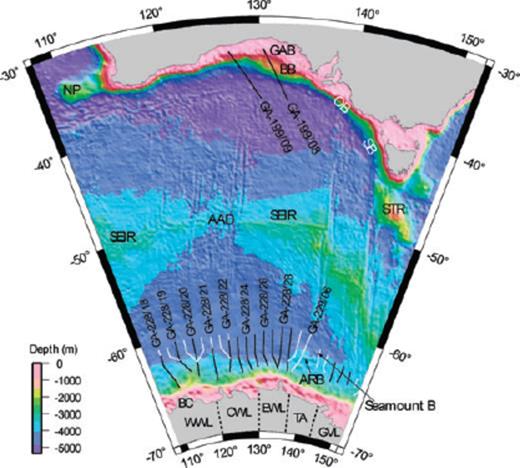
Regional setting of the Wilkes Land margin and major geographic and morphologic features. Profile locations for surveys GA-228 (black) and GA-229 (white) are illustrated on the Wilkes Land margin and for survey GA-199 in the Great Australian Bight (GAB). Seamount B is the location of the dredge samples reported by Yuasa et al. (1997). AAD, Australian-Antarctic Discordance; ARB, Adélie Rift Block; BB, Bight Basin; BC, Budd Coast; CWL, central Wilkes Land; EWL, eastern Wilkes Land; GVL, George V Land; NP, Naturaliste Plateau; OB, Otway Basin; SEIR, Southeast Indian Ridge; SB, Sorell Basin; STR, South Tasman Rise; TA, Terre Adélie; WWL, western Wilkes Land.
Wannesson et al. (1985) noted the presence of a basement high and associated region of shallow bathymetry offshore from Terre Adélie (Fig. 1). They interpreted this high as an ‘anomalous oceanic zone’, partly on the basis of seismic character and the interpretation of a ‘continuous oceanic Moho’ beneath the region and partly due to the interpretation of seafloor spreading anomalies in the region by Cande & Mutter (1982).
Consistent with the interpretation of Wannesson et al. (1985), Eittreim & Smith (1987b) attribute a persistent reflector beneath the outer part of the rift basin to the oceanic Moho and, hence, interpret the zone of ‘elevated basement’ as oceanic crust. Accordingly, Wannesson et al. (1985) and Eittreim & Smith (1987b) suggested that the continent-ocean boundary (COB) was located south or landwards of the ‘elevated basement’. However, the interpretations of Tanahashi et al. (1987, 1997) differ markedly. Tanahashi et al. (1997) reported continental rocks (including granite, gneiss, slate and diorite) dredged from seamounts located seawards of the ‘elevated basement’. Yuasa et al. (1997) also reported in situ peridotite blocks dredged from a seamount with ‘fertile subcontinental characteristics’, inferring that oceanic crust was not being actively produced in this area at the time of seamount emplacement. Tanahashi et al. (1997) therefore interpreted the ‘marginal high’ to be stretched continental lithosphere and suggested that the COB is located seawards of the ‘elevated basement’.
The ‘anomalous oceanic zone/elevated basement/marginal high’ interpreted by previous workers correlates with a block of highly stretched, deeply subsided and extensively faulted continental crust imaged in MCS data from surveys GA-228 and GA-229 (Colwell et al. 2006; Close et al. 2007). Colwell et al. (2006) labelled this region the ‘Adélie Rift Block’ (ARB) and Close (2004) identified its spatial correlation with a region of gravity anomalies atypical for a continental margin and a complete absence of seafloor spreading magnetic anomalies.
Traditionally, the primary constraint on the extent of oceanic crust at rifted continental margins has been provided by magnetic anomaly data. However, in the Australia-Antarctic Basin (AAB), it is not possible to use these data in isolation due to their complexity (Fig. 2).

(a) Location of magnetic profiles and lineations of Chrons 11, 21 and ‘34y’ and the 2500 m isobath. (b) All GA-228 and selected GA-229, JNOC (‘th’) and ‘USNS R/V Eltanin’ (‘EL’) magnetic anomaly profiles across the Wilkes Land margin correlated to a synthetic profile. Filled squares correspond to the lineation previously interpreted as Chron 34y. Chron lineation labels ‘n’ and ‘r’ designate normal and reverse polarity, respectively. Model assumes a 500-m-source layer with its depth fixed at 5.5 km and a remanent magnetization inclination of 75° and amplitude of 4 A m−1. Remanent declination was assumed to be 0° in accord with previous studies (e.g. Weissel and Hayes, 1972). HSR, half spreading rate.
The magnetic anomaly sequence in the southeast Indian Ocean was first interpreted by Weissel & Hayes (1972) in terms of an early Eocene age for continental breakup. A major revision of this age was proposed by Cande & Mutter (1982) who concluded that anomalies 19–22 of Weissel & Hayes (1972) could be better modelled as anomalies 20–34, assuming a slow spreading rate of ∼5 mm yr−1. Accordingly, they revised the age of separation from ∼53 Myr to 86–110 Myr, which corresponds to the long Cretaceous normal polarity epoch.
Tikku & Cande (1999) introduced a new spreading rate model for the Late Cretaceous to early Tertiary. The major departure from earlier models was the introduction of a period of ‘ultra-slow spreading’ (∼1.5 mm yr−1) between anomaly 31o and 24o time (∼68.7–53.3 Ma). They also demonstrated that plate reconstructions using rotation poles based on anomalies 34y, 33o and 32y resulted in ‘significant’ continental overlap in the eastern AAB, and that these anomalies may, therefore, not represent isochrons.
The interpretation of MCS reflection data from the southern Australian margin by Sayers et al. (2001) further revised the Australia-Antarctica breakup age. According to their interpretation, anomaly ‘34y’ (from Tikku & Cande 1999) overlies stretched continental, rather than oceanic crust. On the basis of their interpretation and the magnetic anomaly interpretation of Tikku & Cande (1999), Sayers et al. (2001) suggested that breakup occurred around Chron 33o time (∼79 Ma).
3 Marine Geophysical Data
The first regional, MCS data over the Wilkes Land margin were acquired onboard R/V Geo Arctic by GA Surveys GA-228 and GA-229 during the austral summers of 2000–01 and 2001–02. During these surveys, approximately 9000 km of 36-fold data were recorded on the margin from a 288 channel, 3600 m streamer, using a tuned 60 L airgun array source. The record length was 16 s and the resulting high-quality data provide clear imaging down to the lower crust and, in places, the upper mantle, as well as clear definition of the sedimentary packages.
A total of 19 non-reversed, expendable sonobuoys recorded wide-angle reflection and/or refraction data during surveys GA-228 and GA-229 coincident with MCS transects. All sonobuoy data were modelled at GA using SIGMA ray tracing software (Seismic Image Software Ltd., 1995, unpublished data). A starting model at each refraction station was constructed by depth-converting the interpreted reflection seismic section, using fixed interval velocities estimated from seismic stacking velocities. The model was then iteratively matched to the sonobuoy refraction and wide-angle reflection picks by adjusting layer velocities and depths while, at all times, preserving the layer geometries defined in the seismic reflection data.
Sediment thickness data were compiled by Close et al. (2007) from all the available seismic reflection data available, including the GA, USGS, IFP and JNOC survey data. The velocity model used for the depth conversion of interpreted seismic horizons was based on stacking velocities derived from semblance analysis and velocities derived from the sonobuoy modelling. However, as there has been very limited drilling on the Antarctic margin there are no check-shot surveys available to calibrate these velocities.
4 Magnetic Modelling
We have compared the observed magnetic anomaly profiles to calculated magnetic anomaly profiles of the Wilkes Land margin (Fig. 2). The observed anomalies were computed using the IGRF 2000 model (IAGA, 2000) and have been projected onto a north-south azimuth. The calculated anomalies are based on the geomagnetic reversal time scale of Cande & Kent (1995) and a similar spreading rate model to that assumed by Tikku & Cande (1999). The main difference between our model and that of Tikku & Cande (1999) is an increased spreading rate of 7.5 mm yr−1 from 21y to 22y and the extension of ultra-slow spreading (1.5 mm yr−1) from 22y to 32y. Fig. 2 shows that south of the Southeast Indian Ridge (SEIR), the observed and calculated anomalies compare well, at least for Chron 21 and younger anomalies. The anomaly sequences corresponding to Chrons 11–13, 16–17 and 19–21 are modelled particularly well. Correlating the observed anomaly sequence older than Chron 21, however, is difficult, as the along-strike continuity of the anomalies is extremely poor.
The only common feature of magnetic profiles from the Wilkes Land margin south of Chron 21 is a positive anomaly with an amplitude of ∼200 nT and a wavelength of ∼50–150 km (filled squares in Fig. 2). This anomaly was previously interpreted by Weissel & Hayes (1972) as anomaly 22 and by Cande & Mutter (1982) as anomaly 34y. Although the anomaly does not exhibit a consistent amplitude or wavelength along-strike, it remains the most distinctive magnetic anomaly older than Chron 21.
Off eastern Wilkes Land and Terre Adélie observed anomalies older than Chron 21 are poorly correlated, and there is no equivalent to anomaly 34y of Cande & Mutter (1982). This indicates that breakup was likely not synchronous along the incipient SEIR and that oceanic crust emplacement occurred much later in the eastern sector of the AAB than it did in the central and western sectors. However, due to the uncertainty in identifying the oldest seafloor spreading anomalies in the AAB, we are unable to date the breakup of Australia and East Antarctica with any degree of certainty on the basis of magnetic data alone.
The poor continuity of lineated magnetic anomalies older than the Eocene indicates that either older oceanic crust from the AAB did not acquire a strong thermoremanent magnetization (TRM) at the time of emplacement, or processes have subsequently acted to alter the original TRM. We believe that alteration is the most likely explanation. One possible cause is the slow spreading rate at the SEIR prior to Chron 21, which caused the AAB to remain narrow for a period of tens of million years. During this period young oceanic crust, and possibly even the SEIR, could have been blanketed by sediment derived from the adjacent continents. Hydrothermal alteration of oceanic crust (e.g. Levi & Riddihough 1986) in the AAB from breakup until the Middle Eocene may therefore contribute to the discontinuity in lineated magnetic anomalies and the associated uncertainties in interpreting the age and origin of the observed anomalies.
5 Seismic Data
5.1 Seismic stratigraphy and sediment thickness distribution
Close et al. (2007) identified four megasequences in seismic reflection profile data from the Wilkes Land margin (referred to as MS4, MS3, MS2 and MS1); this paper follows their interpretation and nomenclature. The megasequences are bounded by basement (continental, oceanic and transitional), three regional seismic unconformities (labelled ‘tur’, ‘maas’ and ‘eoc’ in Figs 3 and 4) and the seafloor. On the basis of seismic character correlations with equivalent seismic sequences on the southern margin of Australia, Colwell et al. (2006) and Close et al. (2007) interpreted horizon ‘tur’ as being of early Turonian age, horizon ‘maas’ as Maastrichtian and horizon ‘eoc’ as early Middle Eocene.
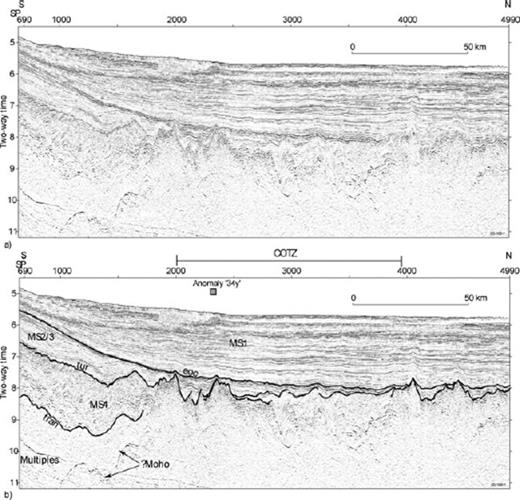
Time migrated MCS profile for line GA-228/24 from central Wilkes Land. (a) Uninterpreted profile and (b) interpreted profile. The prominent unconformities that separate MS1, MS2/3 and MS4 are evident. Modified from Close et al. (2007). See Figs 1 and 2(a) (bold ship-track profiles) for location.

The broad geometries of sequences MS1-MS4 offshore of central Wilkes Land (∼120°–135°E) and the character of the bounding unconformities are illustrated in the MCS profile for line GA-228/24 off central Wilkes Land (Fig. 3). Line drawings of MCS profiles from lines GA-228/18 (western Wilkes Land), GA-228/24 and GA-228/28 (eastern Wilkes Land) are included in Fig. 4 to illustrate the regional variation in sediment thickness, seismic sequence character, depth to basement and crustal structure along the margin.
Close et al. (2007) also produced isochore maps in two-way-time (TWT) for megasequences MS2/MS3 and MS1 and an isochore map of the total post-rift section along the Wilkes Land margin; the total post-rift isochore map is shown here as Fig. 5. The isochores show that the post-rift sediments are generally thick along the margin and in the adjacent deep-ocean basin but are particularly thick in a major depocentre off western Wilkes Land, which they named the Budd Coast Basin (BCB). The BCB contains a maximum observed thickness of 5 s TWT (∼9 km) of post-rift sediments, the major part of which comprises sediments of megasequence MS1, and its location suggests that the sediments were largely derived from a subglacial basin currently occupied by the Totten Glacier.
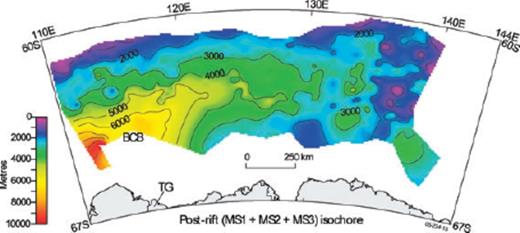
Total post-rift sediment isochore for Wilkes Land, comprising megasequences MS1, MS2 and MS3. BCB, Budd Coast Basin; TG, Totten Glacier. Modified from Close et al. (2007).
5.2 Continental, transitional and oceanic crust
Interpretation of the seismic reflection profile data, together with the sonobuoy refraction and wide-angle reflection data, shows that continental crust underlies the landward (southern) ends of all MCS profiles. The sonobuoy data are summarized in Table 1 and the corresponding locations are illustrated in Fig. 6. Three sonobuoys recorded arrivals with refraction velocities of between 5.4 and 6.6 km s−1 (H, K and R in Table 1 and Fig. 6), coincident with the reflection horizon ‘tran’ (Fig. 3). This is interpreted to indicate the presence of crystalline continental crust below megasequence MS4. Where the Moho is imaged beneath the slope and rise, the continental crust (between the Moho and horizon ‘tran’; e.g. Fig. 3) thins rapidly from ∼10 to <4 km over a distance of ∼80 km. Deeply subsided, stretched continental crust is interpreted to extend for up to 250 km seaward from the shelf break.
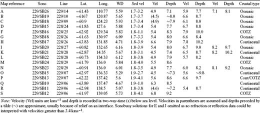
Sonobuoy locations and solutions for surveys GA-228 and GA-229 from Stagg et al. (2005).

Wilkes Land continental margin showing: sonobuoy deployment locations (letters correspond to Table 1); COTZ extents used in this study; alternative COTZ outer limit from Colwell et al. (2006) off western Wilkes Land and magnetic anomaly lineations of Chrons ‘34y’ and 21.
Oceanic crust is interpreted at the seaward ends of all the GA-228 and GA-229 seismic profiles along offshore Wilkes Land. This crust is characterized by a relatively transparent reflection character and a generally rugged, highly reflective upper surface (e.g. Fig. 3, seaward end of the profile). The velocity structure interpreted from refraction modelling is also characteristic of oceanic crust. Refraction velocities from 4.5 to 5.4 km s−1 were modelled from the upper oceanic crust (as interpreted from seismic reflection data), within the average range of normal layer 2 oceanic crust (Bratt & Purdy 1984; White et al. 1992). Velocities of 6.6–6.7 km s−1 were recorded at five sonobuoy locations from the lower oceanic crust, indicating the presence of a distinct oceanic layer 3 (Raitt 1963; White et al. 1992). The thickness of overlying layer 2 crust at these locations ranges from 1.3 to 2.6 km, which is a typical range for this layer (White 1984; White et al. 1992).
Mantle velocities (>8 km s−1) were recorded at only two sonobuoys over oceanic crust (I and N in Table 1 and Fig. 6). The thickness of layer 3 crust at these locations was 1.7 and 3.0 km, significantly less than the average oceanic Layer 3 thickness of ∼4.6 km (Raitt 1963; White et al. 1992). A total crustal thickness of 4.9–5 km is computed at these locations, about 2 km thinner than the average oceanic crustal thickness (not affected by fracture zones and hotspots) of 7.1 km (White et al. 1992). These data conform to previous studies, which found that oceanic crust formed at spreading rates slower than <15 mm yr−1 are significantly thinner than crust generated at faster spreading rates (Muller et al. 1999), and that these total thickness variations are, primarily, a function of changes in layer 3 thickness (e.g. Mutter & Mutter 1993).
Between the seaward edge of thinned and strongly faulted continental crust and the landward edge of seismically distinctive oceanic crust, we have interpreted a broad COTZ that ranges in width from ∼30 to >100 km. The COTZ is characterized by the presence of basement ridges (e.g. SPs 1750–2500, Fig. 3; SPs 4000–4500, Fig. 4c), shallow-crustal discordant bodies and areas of thick pre-rift and syn-rift sediments (e.g. Colwell et al. 2006; Fig. 6.6–5). Overall, the COTZ crust is far more reflective and is more highly structured than normal oceanic crust.
The COTZ can be clearly identified along the margin except off western Wilkes Land, where extremely thick and highly reflective post-rift sediments limit the seismic penetration of the underlying crust. Colwell et al. (2006) interpreted a very broad (∼175 km) COTZ in this area, and the outer limit of their COTZ is located immediately landward of Chron 21 (Fig. 6). O'Brien & Stagg (2007) also followed that interpretation, while noting that the outer edge of the COTZ (their COB) was interpreted in the most seaward possible location. Based on an alternate interpretation of seismic reflection data and evidence from interpreted seafloor spreading magnetic anomalies, Close (2004) delimited the outer limit of the COTZ a substantial distance (up to 100 km) landward of Colwell et al. (2006). Here we follow the COTZ interpretation of Close (2004) (Fig. 6).
The outer limit of the COTZ is located ∼200 km from the shelf break along western and central Wilkes Land (Fig. 6). However, off eastern Wilkes Land/Terre Adélie, in the region of the ARB, the outer limit of the COTZ is interpreted at more than 400 km seaward of the shelf break. This interpretation is supported both by the dredge samples of continental rocks collected on JNOC survey TH-95 (Tanahashi et al. 1997; Yuasa et al. 1997) and by the seismic reflection character that shows a large thickness of obvious rift-stage sediments at this location (Fig. 7).

Detailed section from survey line GA-229/06 across the northern flank of the Adélie Rift Block (location shown in Fig. 6). The reflector patterns and faulting evident below the ‘maas’ horizon confirm that the ARB does not comprise oceanic crust.
The basement highs within the COTZ may represent shallow, intrusive igneous bodies associated with Jurassic magmatic activity. However, it is more likely that they represent peridotite ridges or exhumed mantle, as proposed by Close (2004) and Colwell et al. (2006). This interpretation is supported by the dredging of in situ peridotite rocks of interpreted continental affinity (Yuasa et al. 1997), in close proximity to continental basement rocks dredged from low-relief seafloor highs off Terre Adélie (Tanahashi et al. 1997). Off central and eastern Wilkes Land the location of basement ridges coincides with the seaward termination of the Moho horizon in MCS data. A lack of typical mantle velocities also characterizes the transition zone crust of the Iberian Abyssal Plain margin (Dean et al. 2000). If the basement ridges observed off the Wilkes Land margin are in part exhumed mantle, then they are likely to be serpentinized peridotite ridges similar to those interpreted off the Iberian margin. Sayers et al. (2001) have similarly interpreted a basement ridge on the conjugate southern Australian margin as a peridotite ridge.
6 Gravity Anomalies and Gravity Modelling
6.1 Free air anomaly data and the continental margin edge effect
Fig. 8 illustrates the satellite-derived free air anomaly (FAA) data on the Wilkes Land margin (Sandwell & Smith 1997) and ship-track FAA data from surveys GA-228 and GA-229. We have used the geopotential coefficient model of Rapp & Pavlis (1990) to remove the long wavelength (spherical harmonic degree and order 12 and lower) negative FAA associated with the Australia-Antarctic discordance (Weissel & Hayes 1972; Veevers 1982) from the satellite-derived and ship-track data.
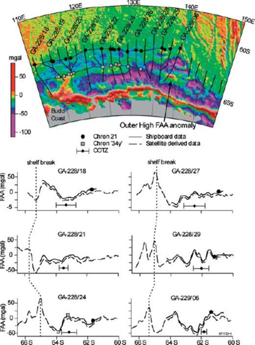
(a) Marine gravity anomaly field for the Wilkes Land margin (Sandwell & Smith, 1997) with Chrons 21 and ‘34y’. (b) Survey GA-228 and GA-229 shipboard (solid) and satellite derived (dashed) FAA data.
One of the most prominent features of the marine free-air gravity field is the ‘edge effect’ observed at continental margins, which typically comprises a peak over the shelf break and a trough over the continental slope/rise. This high-low ‘couple’ is observed along much of the Wilkes Land margin. The edge effect high exceeds 60 mGal in the eastern sector only and the low is typically no more negative than −40 mGal. Profiles extracted from the satellite-derived FAA field (Fig. 8), coincident with GA-228 survey lines and extended south to the Wilkes Land coast, illustrate the variation in and the variability of the edge effect anomaly along the margin. However, it should be noted that although the qualitatively good correlation between satellite-derived and shipboard FAA data is evident, the fidelity of the satellite-derived FAA data is questionable farther to the south as the extent of permanent sea ice is approached. This is due to the scattering effects of the sea ice and the relatively sparse satellite coverage at high latitudes relative to low latitudes (McAdoo & Laxon 1997).
The central Wilkes Land sector is characterized by a generally consistent edge effect anomaly. To the west and east, however, significant departures are evident. In the western sector, at the prominent Budd Coast headland (∼112°E), the absence of a distinct morphologic shelf break partially explains the discontinuity in the edge effect anomaly (i.e. the break in the peak at ∼111°E and the break in the trough at ∼115°E). The Budd Coast margin is also characterized by a number of large-relief sediment ridges extending from the upper continental slope, broadly oriented orthogonally to the margin. These sedimentary features correlate with positive FAA, indicating that they are, at least in part, uncompensated.
Off the eastern Wilkes Land/Terre Adélie sector (∼132°–142°E), the relatively broad edge effect low typical of central and western Wilkes Land is replaced by an ‘outer high’ and the low is split into two limbs encompassing the outer high (Fig. 8). This region is coincident with the continental fragment of the ARB. This margin sector is characterized by much thinner post-rift sediments, decreasing to less than 1 km thick in some areas.
6.2 Gravity modelling—a process oriented approach
The observed FAA at a continental margin can be considered as the result of all the processes that have shaped it through geological time. The ‘process-oriented’ method of modelling gravity anomalies (e.g. Watts 1988 in 2-D; Stewart et al. 2000 in 3-D) attempts to compute the gravitational contribution of rifting and sedimentation, with the aim of better understanding the contributions of other processes, such as magmatism (e.g. Watts & Fairhead 1997).
The method involves three main steps. First, sediments are flexurally backstripped and the depth to basement in the absence of sediment loads is calculated (Watts 1988). The present-day water depth (which can be considered as the unfilled portion of the depositional basin) is added to the flexural backstrip to determine the total tectonic subsidence (TTS; Sawyer 1985). The TTS depends on the Te, which is a measure of lithospheric rigidity and, therefore, a proxy for its strength. A high Te estimate typically results in a deeper TTS and vice versa. Second, the TTS is used to restore the crust and mantle structure at the time of rifting by assuming a pre-rift crustal thickness with a zero-elevation upper surface and a local (e.g. Airy) or regional isostatic compensation (e.g. Watts 2001).
The final step is to compute the gravity effect of the restored crustal structure (the rift anomaly) and the sediment load and its compensation (the sediment anomaly) and compare their sum to the observed FAA. The rift anomaly consists of a negative, associated with the TTS and the replacement of crust by water, and a positive, associated with crustal thinning and the replacement of crust by mantle. The sedimentary sequence generates a positive anomaly associated with the sediment load and flanking negative anomalies associated with both the replacement of crust by sediment and the associated displacement of mantle by crust.
Fig. 9 shows the results of applying the process-oriented method to line GA-228/18. This line, which is in the western sector, traverses some of the thickest sediments encountered on the Wilkes Land margin. The rifting anomaly shows a typical high-low ‘couple’ that reflects the initial configuration of the margin, whereas the sediment anomaly shows a broad positive anomaly that correlates with the thickest sediments. The anomalies have been computed assuming the zero-elevation crustal thickness and the densities of the crust, sediment and mantle summarized in Table 2. The sum anomaly depends on the value of Te that is assumed. For example, Te = 5 km predicts an anomaly that is relatively small in amplitude compared with that observed, whereas Te = 45 km predicts an anomaly that is too large. The best fit to both the amplitude and wavelength of the observed anomaly is for Te = 30 km (Fig. 9).
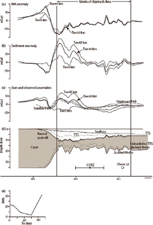
Process-oriented modelling demonstrated for line GA-228/18 for Te = 30 km (solid black). (a) The rift anomaly. (b) The sediment anomaly. (c) Comparison of the observed ship track (short dash) and satellite-derived (long dash) FAA data to the calculated sum anomaly. (d) Loaded and unloaded post-rift crustal structure based on TTS derived assuming Te = 30 km (i.e. crust-mantle boundary is estimated and not constrained by seismic data in this example). (e) The rms misfit as a function of Te illustrating a minimum for Te = 30 km.
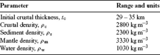
Parameters utilized in process-oriented modelling.
Although there is good agreement between observed and calculated FAA along line GA-228/18, we found it difficult to determine Te along lines over other margin sectors where the sediment thickness is smaller. However, Fig. 10 demonstrates that we were able to provide some constraints on the Te structure. The figure shows, for example, that Te = 5 km cannot explain the amplitude of the edge effect along lines GA-228/24 and GA-228/28 over the central and eastern sector. The high requires Te = 30 km, or greater, to explain both it and the flanking seaward low. The edge effect therefore fits the calculated anomalies reasonably well; however, the fit in the region of the COTZ is poor. We believe this is due to the much thinner sedimentary section and to the rugged topography of the COTZ basement (which comprises several large-amplitude ridges). However, even in this region where the rms error is relatively insensitive to Te, we can see qualitatively that the gravity anomaly is best fit by Te = 30 km.
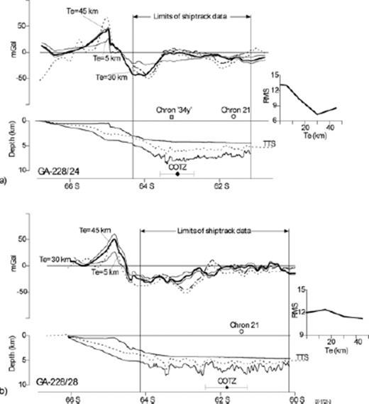
Process-oriented modelling results for (a) Line GA-228/24 and (b) Line GA-228/28. Gravity panels include ship-track data (dashed), satellite derived data (dotted) and modelling results for three Te values (5, 30 and 45 km as labelled). Crustal panels include the seafloor and the base of the post-rift sediments (solid) and the TTS (dashed).
The process-oriented modelling in Figs 9 and 10 implies a distinct crust and mantle structure that can be verified by seismic data. Unfortunately, Moho reflections in seismic reflection data and mantle velocities in sonobuoy refraction data on the Wilkes Land margin are limited to central and eastern Wilkes Land and Terre Adélie.
Fig. 11 illustrates the spatial correlation of the Moho interpreted from MCS data and the flexed Moho calculated from the modelled TTS, assuming an initial crustal thickness (tc) of 32 km, for line GA-228/28. Similar correlations are evident for lines GA-228/22, GA-228/24, GA-228/25, GA-228/26, GA-228/27 and GA-228/29. Additionally, a close correlation of sonobuoy-derived Moho depth and model derived Moho depth is also observed on lines GA-228/25, GA-228/27 and GA-228/29.
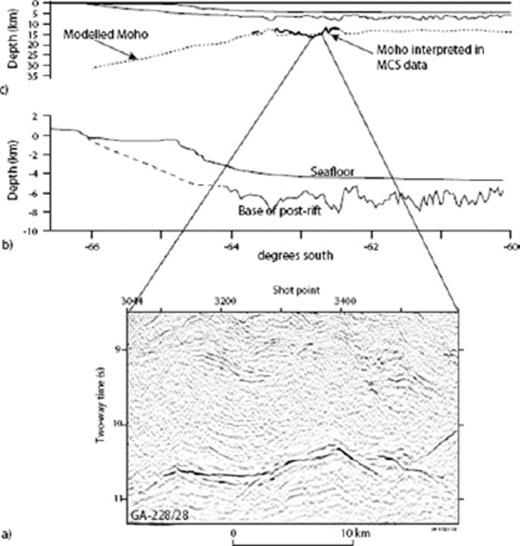
Crustal structure and seismic detail for line GA-228/28. (a) MCS data illustrating Moho reflections between 10–11 s TWT. (b) Post-rift sedimentary sequence (dashed line based on non-GA survey data). (c) An example of the close spatial correlation between Moho depths derived from backstripping and process-oriented gravity modelling (i.e. estimated) and constraints on Moho depth from MCS data (i.e. measured).
The best fitting tc of 30–32 km for eastern Wilkes Land and Terre Adélie is less than the assumed tc for western Wilkes Land of 35 km. This reflects the larger TTS and thick sediment accumulation for western Wilkes Land. If tc = 32 km is assumed for western Wilkes Land, then negative stretching factors result, which is untenable. Without more detailed refraction data, it is not possible to conclude whether the thickness of unstretched crust changes along the margin, or if the implicit modelling assumptions are in error. For example, if the initial subsidence associated with crustal thinning was regional and not Airy compensated, then a lower tc is tenable for western Wilkes Land. However, Collins et al. (2003) inferred that the continental crust of the conjugate Australian margin was thinner (i.e. a shallower depth to the Moho) for Tasmania (broadly conjugate to Terre Adélie and George V Land) relative to southwest Australia (conjugate to western Wilkes Land).
We have assumed thus far a zero strength lithosphere during rifting. The effects of incorporating finite strength during rifting have been considered by a number of authors (e.g. Cochran 1973; Weissel & Karner 1989), as has the possibility of a necking depth being important in the rifting process (Kooi et al. 1992). However, there is no consensus on how lateral and vertical variations in lithospheric strength affect the rifting process, and the importance of other factors such as the geotherm and strain rate have been demonstrated to be of equal, if not greater importance (e.g. Bassi 1995; Buck et al. 1999). The effect of incorporating strength during rifting, using the method of Stewart et al. (2000), was tested for the Wilkes Land margin. The results of these tests indicate that finite strength during rifting is not required to explain the FAA, and therefore that the assumption of local or Airy isostasy during rifting is a reasonable one that is consistent with the gravity data (Close 2004).
Process-oriented gravity modelling demonstrates that flexural compensation of continental margin sediments off Wilkes Land is important and indicates that the lithosphere is characterized by a Te of ∼30 km, which is relatively high for a rifted margin. Additionally, the Wilkes Land margin does not appear to be segmented with reference to its long-term strength, and variations in the edge effect anomaly are primarily functions of morphology and sediment distribution. However, the persistence of flexural isostatic anomalies (i.e. the anomalies remaining after subtracting the calculated sum anomaly from the observed FAA) indicates that process-oriented modelling cannot fully account for the density distribution within the Wilkes Land margin lithosphere. Where distinct flexural isostatic anomalies occur, it is possible to further investigate their origin and nature by modelling discrete bodies within the crustal section, which had previously been assumed to be homogenous.
7 Coincident Gravity and Magnetic Data Modelling
Although process-oriented modelling accounts for much of the amplitude and wavelength of gravity anomalies observed on the Wilkes Land margin, there are notable discrepancies within the COTZ that correlate spatially with high-relief basement ridges on the MCS lines (e.g. GA-228/22, GA-228/23, GA-228/26, GA-228/27 and GA-228/29). Coincident, positive magnetic anomalies are also observed on lines GA-228/22 and GA-228/23.
Fig. 12 shows the flexural isostatic anomaly (Te = 30 km) and the coincident magnetic anomaly on line GA-228/22 over the COTZ. The figure demonstrates that the anomaly pair can be explained by a relatively dense body, extending from the modelled Moho (i.e. from process-oriented gravity modelling) landward of the COTZ to the base of the post-rift section, with a magnetized upper section. A contrasting magnetic susceptibility is applied to the upper section of the ridge, as magnetization is proportional to degree of serpentinization, which we assume is greater at shallower depths.
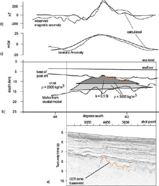
(a) MCS data from the COTZ on Line GA-228/22 with orange horizon marking top of basement ridge. (b) Crustal structure from process-oriented modelling and modelled body geometry (grey shade) with density (ρ) and magnetic susceptibility (k) as labelled (magnetic body is the dark grey upper section of the larger dense body). The orange horizon is as for panel (a) converted to depth. (c) Isostatic anomaly (Te = 30 km) and calculated gravity anomaly for light grey body in (b). (d) Observed magnetic anomalies compared with calculated anomalies assuming induction only for the dark grey body in (b). Calculated magnetic anomalies are assumed to be due to induction in the present-day geomagnetic field only (i.e. very low Königsberger ratio) and ambient magnetic field properties assumed are as for the present day Wilkes Land margin, that is, field strength = 66 000 nT, inclination = −80° and declination = −3° (IAGA, 2000).
We constrained the depth to the upper surface of the body using the MCS data, which also show the characteristic ridge topography and seismic character. The modelled density contrast is 200 kg m−3, which implies a density of 3000 kg m−3 for the basement ridge, as a crustal density of 2800 kg m−3 was assumed for the calculation of the flexural isostatic anomaly. The modelled susceptibility is 0.1 SI, which is within the range of measured values (0.01–0.15 SI) determined by Oufi & Cannat (2002), based on the analysis of variably serpentinized peridotite samples from Offshore Drilling Program (ODP) drilling.
We speculate that the relatively dense and high susceptibility body within the COTZ is a serpentinized peridotite ridge. A density of 3000 kg m−3 would correspond, for example, to ∼35% serpentinization (Horen et al. 1996). Unfortunately, the susceptibility does not vary systematically with the degree of serpentinization (Oufi & Cannat 2002). Instead, susceptibility remains low in partially serpentinized peridotites and then increases rapidly as a threshold of ∼75% alteration is reached.
Support for our interpretation comes from the recovery of in situ peridotites, with geochemical characteristics typical of continental mantle lithosphere, dredged from a seamount offshore Terre Adélie (Yuasa et al. 1997). The ridge is therefore interpreted to be analogous to the drilled mantle peridotite ridges on the West Iberia margin, which were interpreted to have been exhumed during a similarly non-volcanic, slow-rate rifting event (Pinheiro et al. 1996).
The magnetic anomaly in Fig. 12 corresponds in position with the ‘34y’ lineation discussed earlier (see Fig. 2). We therefore support the conclusions of Tikku & Cande (1999) and Sayers et al. (2001) that ‘34y’ is not a seafloor spreading anomaly. Our results suggest that the lineation is associated with serpentinized mantle peridotites. This, together with the lack of an easily correlatable magnetic anomaly sequence prior to the Eocene, makes it difficult to constrain the timing of the breakup and the onset of seafloor spreading between Antarctica and Australia, using magnetic anomalies alone.
8 Discussion
8.1. COTZ structure and crustal thinning
The Wilkes Land margin is characterized by low extension rates, which contribute to low melt generation, a key factor in allowing mantle exhumation (Pérez-Gussinyé 2001). However, a detachment surface at the crust-mantle boundary, similar to that suggested by Pérez-Gussinyé. (2001), for which there is evidence in seismic reflection and refraction data at the Iberian margin (Krawczyk et al. 1996), is not apparent in the seismic data from the Wilkes Land margin. If a décollement surface is absent, it indicates that mantle exhumation may occur through excessive thinning in the absence of magmatism.
A further factor important in the serpentinization and exhumation of the upper mantle is the amount of crustal and mantle extension (Pérez-Gussinyé 2001). High stretching factors (β ≥ 3–4, where β is the amount of crust and mantle extension) are important for the formation of deep crustal penetrating faults that allow conduits for sea water to cause serpentinization of the upper mantle.
The β distribution at rifted margins is an important constraint on dynamic models (e.g. Bassi 1991, 1995). It controls the amount of lithosphere thinning, and hence heating, at conjugate margin pairs, which, in turn, determines the degree to which rifting is a symmetrical or asymmetrical process (Buck et al. 1999). Additionally, estimates of β are integral to inferring the strain rate during rifting, a parameter that is believed to strongly influence the final width of extended continental crust (e.g. Bassi 1995).
We have used process-oriented gravity modelling, together with the available seismic reflection and refraction constraints to estimate the amount of extension across the central sector of the Wilkes Land margin. Fig. 13 shows β as a function of distance from the landward limit of the COTZ defined from MCS data (Fig. 6). The figure shows that the total width of extended continental crust is ∼350 km, and the distance from the shelf-break to the COTZ is ∼150–200 km. β increases approximately linearly from 1 at the southern limits of the analyses, to ∼2.5, 100 km landward of the COTZ. A sharp increase in β occurs towards the COTZ, and maximum values of ∼5 are attained at or just landward of the COTZ.
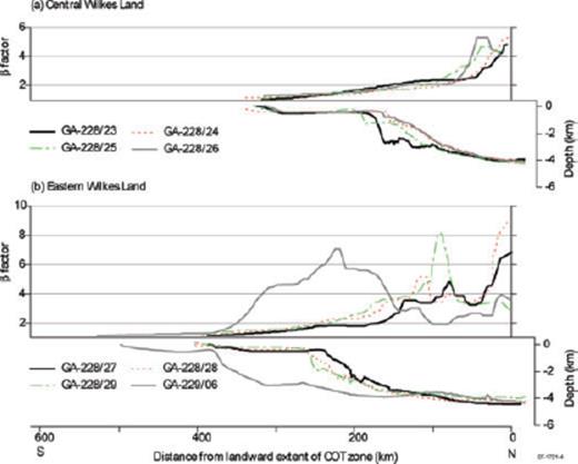
Degree of crustal stretching, β, as a function of distance from the landward limit of the COTZ for (a) central, and (b) eastern Wilkes Land. Bathymetry profiles (lower panels) are from ship track and GEBCO 1 × 1 min data (IOC et al. 2003).
The pattern of crustal thinning in the eastern Wilkes Land and Terre Adélie margin sector is far more variable than in the west. Lines GA-228/27 and GA-228/28 exhibit a relatively similar pattern to the central Wilkes Land transects, except that β values exceed 6 and 8 on these lines, respectively. Both lines also indicate a zone of increased crustal thinning (β > 4) at ∼100 km landward of the COTZ. The peak value of β on Line GA-228/29 (∼8) is coincident with this zone of increased crustal thinning, not at the landward limit of the COTZ. The total width of extended continental crust for lines GA-228/27–GA-228/29 is almost 400 km and the shelf-break to COTZ distance is 225–275 km.
The β for line GA-229/06, across the ARB, is markedly different from margin sector transects to the west. The distance from the shelf-break to COTZ on this line is almost 400 km. Additionally, the width of crust where β > 4, almost 200 km, is also much greater than in other margin sectors, and the region of maximum β is more than 150 km landward of the COTZ. This indicates that the ARB is an anomalous zone of stretched continental crust that was likely a continuation of the Australian continental crust as the rift initiated, but as the slow spreading Southeast Indian Ocean Ridge finally broke through the ARB, the locus of extension transferred north leaving the ARB attached to Antarctica and a point of massive thinning landward of the eventual breakthrough of oceanic crust. This is consistent with the interpretation of Colwell et al. (2006).
In Fig. 14 the β distribution calculated for the central Wilkes Land margin (line GA-228/24) is compared with other margins, including South Africa, Nova Scotia, Gabon, eastern USA, Brazil (Campos Basin), Goban Spur, Carolina and the Valencia Trough (western Mediterranean). The Valencia Trough and eastern USA curves are based on gravity modelling, flexural backstripping and crustal balancing studies (Watts 1988; Watts & Torné 1992). The South Africa curve is based on flexural backstripping (Young 1992). The Carolina, Brazil, Nova Scotia and Goban Spur curves (Watts & Fairhead 1997) were obtained by flexural backstripping previously published seismic reflection profile data (Beaumont et al. 1982; Hutchinson et al. 1983; Mohriak et al. 1990; Horsefield 1991). Results from the Otway Basin are based on the refraction data of Finlayson et al. (1998), those from West Iberia are based on flexural backstripping (T. Cunha, unpublished data, 2004) and those from the Great Australia Bight (GAB) margin are from this study. Fig. 14 shows that the Wilkes Land margin is an example of a wide rift. The results from the West Iberia, Nova Scotia and Gabon margins indicate that crustal thinning can occur over a broad region, up to 300 km landward of oceanic crust. These results are similar to the observed crustal thinning pattern for eastern Wilkes Land and Terre Adélie.
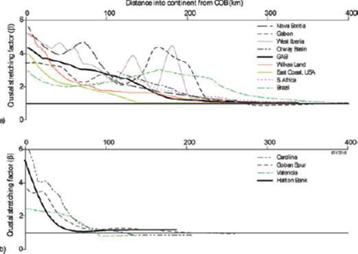
Comparison of crustal extension, as determined from a variety of methods, as a function of distance from the estimated location of oceanic crust. (a) Rifts characterized by broad zones of extension, and (b) narrow rifts where extension is focused within 100 km. The results from West Iberia and Gabon indicate that the locus of extension can occur at large distances from the point of eventual crustal rupture. See text for details of data sources.
The reasons for the large variations in the distribution of crustal thinning at rifted margins are not clear. Bassi et al. (1993) showed, for example, that the width of stretched continental crust on passive margins depends strongly on the initial thermal conditions. Narrow margins, such as the Flemish Cap margin could be produced using models of a thick, cold lithosphere, even after relatively small amounts of extension. Wide margins such as the Orphan Knoll margin, on the other hand, could be produced using models of thin, hot lithosphere. Buck et al. (1999), however, argued that narrow rifts do not need a pre-existing weakness, and that necking, magmatic addition and cohesion loss on faults are all ways that rifting may be localized in narrow zones. Wide rifts, on the other hand, are produced by delocalizing effects such as viscous flow, crustal buoyancy and flexure. Finally, Davis & Kusznir (2002) have argued that rifting does not produce narrow or wide margins but a continuum which ranges from ∼50 to ∼500 km. This emphasizes that a number of factors must be involved in rift margin formation.
8.2 Conjugate margin structure and evolution
The Southern Rift System (SRS; Stagg et al. 1999) of southern Australia extends for more than 4000 km from the Naturaliste Plateau in the west to the South Tasman Rise in the east (Fig. 1). The SRS contains several major depocentres, including the Bight, Otway and Sorell Basins. The sedimentary fill is interpreted as predominantly Late Jurassic and Cretaceous age, with the margin being largely sediment-starved during the Cenozoic, in sharp contrast to the Wilkes Land margin. The boundary between the rift and post-rift sediments of the Bight Basin is interpreted at the base of the Tiger Super-sequence (Turonian) of Totterdell et al. (2000).
We have used the process-oriented modelling method on two lines from GA survey 199 (GA-199/08 and GA-199/09) across the Bight Basin (Fig. 1). The parameters utilized were similar to those used for Wilkes Land (see Table 2) except that tc = 33 km. A lack of seismic refraction and/or reflection data that images the Moho in this region prevents tc from being constrained independently.
The model results illustrate that line GA-199/08 is sensitive to variations in Te (Fig. 15). We attribute this to the thick (>5 km) post-rift sediment thickness. Modelling with low Te (i.e. ≤ 10 km) underestimates the magnitude of the positive anomaly over the thickest sediments and overestimates the magnitude of the edge effect high. Conversely, for high Te (i.e. ≥ 30 km) the edge effect high is underestimated, and the high over the thickest sediments is overestimated (along with the gravity low seaward of this high). However, Te = 15 km yields a good overall fit between calculated and observed anomalies.
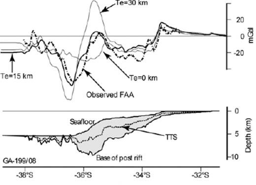
Bathymetry, base of post-rift sediments and TTS (lower panel) and process-oriented modelling results (upper panel) for line GA-199/08. Observed FAA data (dashed) are well fit by the Te = 15 km modelled profile (solid).
The bathymetry of the Wilkes Land and southern Australian margin differs with respect to the morphology of the continental shelf and also in respect to the absolute depth of the marginal abyssal plain (Fig. 1). The abyssal plain off southern Australia reaches depths of over 5250 m, whereas the typical depth, at the equivalent distance from the shelf-break, off Wilkes Land is ∼4750 m.
Although the seafloor is deeper off southern Australia, MCS data from surveys GA-228 and GA-199 illustrate that basement actually is deeper off Wilkes Land (Fig. 16a). Comparing the backstripped basement surfaces (i.e. the TTS; Fig. 16b), the sediment-corrected basement depths are comparable across lines GA-228/22 and GA-228/23 and GA-199/09. However, the TTS on lines GA-228/26 and GA-228/27 is some 1500 m ‘shallower’ than the conjugate line GA-199/08. The large calculated TTS may have contributed to the greater thickness of syn- and post-rift sediments observed in the Ceduna Subbasin, by producing greater accommodation space during the early rift stage.
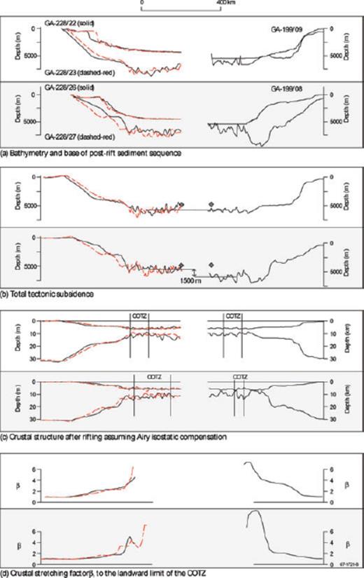
Comparison of a range of observed and derived parameters for the central Wilkes Land and Bight Basin conjugate margins. Profiles are compared landwards of anomaly 20. Line labels for (b)–(d) are as in (a). TTS, crustal structure and β in (b)–(d) are calculated assuming a Te of 30 km for the Wilkes Land transects and 15 km for the Bight Basin transects. Solid diamond symbols in (b) are the predicted depth of Chron 20 (∼43 Ma) aged oceanic crust based on Parsons & Sclater (1977).
Because of the lack of constraint on Moho depth on the southern Australian margin, it is difficult to determine the accuracy of the calculated crustal stretching factor (β) profiles (Fig. 16d). Therefore, it is also difficult to determine the degree of symmetry in extension across the margins. Broadly, extension increases linearly towards the COTZ along lines GA-228/22 and GA-228/23 and GA-199/09, whereas across lines GA-228/26 and GA-228/27 and GA-199/08, a sharp increase in β is observed towards the COTZ.
The FAA across this conjugate margin pair is not symmetric (Fig. 17a) due to the differences in the sediment distribution and morphology that are observed at these margins. There is also a very poor correlation in the magnetic anomaly profiles between lines GA-228/26 and GA-228/27 and GA-199/08 (Fig. 17b). However, a better correlation between lines GA-228/22 and GA-228/23 and GA-199/09 is evident. This is not surprising given that similar problems in identifying anomalies older than Chron 21 exist on the southern Australian margin (Veevers 1986; Tikku & Cande 1999).
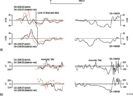
Comparison across the central Wilkes Land and Bight Basin conjugate margins of (a) FAA ship-track data supplemented by satellite derived FAA data landward of the limit of ship-track data (Sandwell & Smith, 1997) and (b) magnetic anomaly data. Profiles are compared landwards of anomaly 20.
The large-amplitude positive magnetic anomaly on lines GA-228/22 and GA-228/23, attributed here to serpentinized upper-mantle peridotite ridges, is mirrored at a similar distance landward from anomaly 20 on line GA-199/09. This magnetic anomaly corresponds to a positive FAA (Fig. 17d) and the location of the basement ridge interpreted by Sayers et al. (2001) as a serpentinized peridotite ridge. This symmetry indicates that the magnetic anomaly lineations previously attributed to Chrons 22 (Weissel & Hayes 1972) or 34 (Cande & Mutter 1982) likely have a common origin but not one that is associated with normal seafloor spreading.
In summary, our data suggest that the GAB and Wilkes Land margins are broadly symmetric, consistent with the interpretation of Stagg et al. (2005). The total width of extended continental crust on each margin is comparable, as are the basement depths when corrected for sediment loading. Previous studies, however, have interpreted the conjugate margin pair as asymmetric and the product of a mixed-mode simple and pure shear extension mechanism (Etheridge et al. 1989; Lister et al. 1991). According to these studies, the Australian margin is an ‘upper plate’ margin whereas the opposing Wilkes Land margin is a ‘lower plate’ margin. However, we see no evidence in our MCS data for upper-crustal detachment surfaces as predicted by the asymmetric rifting model (e.g. Wernicke 1985). We therefore concur with Sayers et al. (2001) and Stagg et al. (2005) in interpreting this margin pair as broadly symmetric and the product of lithosphere-scale pure shear.
8.3 Te and the strength of extended continental lithosphere
The Te of rifted margins is a useful parameter that reflects their long-term, steady state, thermal and mechanical evolution. In other regions, estimates range from a low of ∼5 km for the Valencia Trough (Watts & Torné 1992) and Baltimore Canyon Trough (Watts 1988) margins, through intermediate values at the New Zealand-Western Platform margin (Holt & Stern 1991), to a high of 40–60 km for the West Greenland and Labrador Sea margins (Keen & Dehler 1997). As pointed out by Karner & Watts (1982), Te at rifted margins reflects the average response of the lithosphere to sediment loading rather than at a particular time since rifting. Thus, average values may be low if the sediment accumulation rate was high early in margin evolution when the lithosphere was relatively hot and, hence weak, and high if the rate was high later in margin evolution when the lithosphere was relatively cool, and hence strong. This assumes that sedimentation is concentrated in the marginal basin and is not distributed uniformly throughout the ocean basin, as it is the change in loads at wavelengths relevant to flexure that is critical to the method used herein. Other factors that might influence Te are the pre-existing thermal and mechanical properties of the rifted lithosphere, thermal blanketing and increases in the sediment load and curvature of flexure (e.g. Watts 2001), which may lead to yielding.
Of particular interest to determining the relationship between Te and the age since rifting would be the case of discrete loading events on conjugate rifted margins. The Wilkes Land and GAB margins are unusual in that they do have highly divergent sediment loading histories. During the mid-Tertiary the Wilkes Land margin was subjected to large sediment loads, whereas the GAB margin was largely sediment-starved. Process-oriented modelling indicates that the Wilkes Land margin is associated with an average Te of 30 km, whereas the GAB margin is associated with an average Te of ∼15 km. The low Te interpreted for the GAB margin therefore indicates that immediately following rifting and through the Late Cretaceous, the lithosphere was relatively weak. However, the high Te interpreted for the Wilkes Land margin indicates that the lithosphere was relatively strong by the mid-Tertiary, when the major sediment load was emplaced. The asymmetry of the Wilkes Land and GAB margins, in terms of their Te, may not reflect differences in their initial structure, rather it demonstrates that Te may have increased through time.
Fig. 18 summarizes the results from the Amazon fan, the Bay of Bengal, the Taiwan foreland and the GAB-Wilkes Land margins. The figure shows that Te generally follows the depth of the 450 °C isotherm based on cooling plate models, suggesting that rifted continental lithosphere regains its strength as it cools following a heating event. This result is in accord with the yield strength envelope considerations of Pérez-Gussinyé. (2001) and the numerical modelling results of Burov & Poliakov (2001), who suggest that lithospheric rigidity initially decreases during early stages of the syn-rift but regains its strength during the later stages of the syn- and post-rift interval. It is difficult to assign a single controlling isotherm to the Te data, but Fig. 18 suggests that a similar controlling isotherm of 450 °C, as describes oceanic flexure data, is in accord with the data.
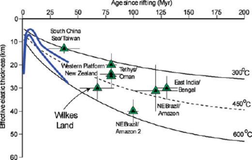
Plot of Te as a function of elapsed time between rifting and load emplacement (for discrete loads) on rifted continental margin lithosphere. Blue lines are the predictions of Burov & Poliakov (2001) based on numerical modelling. Estimates for NE Brazil/Amazon and NE Brazil/Amazon 2 from Rodger et al. (2006), for East India/Bengal from Krishna et al. (2000), for Tethys/Oman from Ali & Watts (in press), Western Platform New Zealand from Holt & Stern (1991) and for South China Sea/Taiwan from Lin & Watts (2002).
Our results do not explain why some old margins, such as the Baltimore Canyon Trough, have a low Te, and therefore rather than regaining their strength have apparently remained weak since rifting. Wyer & Watts (2006) have recently shown that the East Coast US margin is highly segmented with respect to its Te structure, and therefore only segments of the margin, such as the Baltimore Canyon Trough, are weak. They showed that the weak segments correlate with high β and, significantly, high curvatures, which could lead to yielding. We believe therefore that the low values at the Baltimore Canyon Trough are probably due to yielding, which acts to reduce the Te from what it would otherwise be based on age since rifting.
9 Conclusions
We draw the following conclusions from this marine geophysical study of the Wilkes Land rifted margin:
- (1)
Post-rift sediments up to 5 s TWT (∼8–9 km) thick are evident in seismic reflection data on the Wilkes Land margin. The post-rift sediments can be divided into two major post-rift sequences separated by a regional unconformity. The unconformity is interpreted to be Eocene in age (∼50 Ma) on the basis of correlations with the southern Australian margin.
- (2)
The COB trends subparallel to the coastline, except off eastern Wilkes Land and Terre Adélie where it forms a seaward salient of ∼200 km. The salient, which is underlain by stretched continental crust and pre- and syn-rift sediment, is interpreted to represent a deeply subsided marginal plateau.
- (3)
The magnetic anomaly, which previous workers have interpreted as seafloor spreading Chron 34 (the Cretaceous Long Normal Quiet Zone), coincides with the COTZ and is therefore unlikely to have formed by normal processes of seafloor spreading. Integration of the gravity and magnetic anomaly modelling with the MCS data indicate that the lineation is caused by one or more ridges of exhumed, partly serpentinized mantle peridotite.
- (4)
Process-oriented gravity modelling indicates that the lithosphere that underlies the Wilkes Land margin is characterized by Te∼30 km, whereas the conjugate southern Australian margin is characterized by a Te of ∼15 km. We attribute the relatively high Te modelled on the Wilkes Land margin to a relatively recent, glaciation-induced sediment load that was emplaced on lithosphere that increased its long-term strength with time. Therefore, the asymmetry of the Wilkes Land and GAB margins, in terms of their Te, may not reflect differences in their initial structure, rather it demonstrates that Te may have increased through time.
- (5)
Despite the apparent asymmetry in Te structure, the Wilkes Land and southern Australian margins appear to be broadly symmetric with regards to width of extended continental crust and inferred crustal structure.
- (6)
A consistent pattern of crustal thinning is evident for central Wilkes Land. A total width of extended continental crust of ∼350 km is observed. In contrast, the pattern of crustal thinning on the eastern Wilkes Land and Terre Adélie margin is far more variable, where the total width of extended continental crust is almost 400 km, and across the ARB, is over 500 km. This suggests that the ARB is an anomalous zone of stretched continental crust that was likely a continuation of the Australian continental crust as the rift initiated, but as the slow spreading SEIR finally broke through the ARB, the locus of extension transferred north, leaving the ARB attached to Antarctica and a point of massive thinning landward of the eventual COB.
Acknowledgments
The GMT software of Paul Wessel and Walter Smith was widely used for computation and figure drafting. Figure drafting was assisted by S. Mezzomo of Geoscience Australia. The authors acknowledge the helpful reviews of J. Hopper, T. Minshull and an anonymous reviewer. HMJS publishes with the permission of the Chief Executive Officer, Geoscience Australia. This research was supported by a Rhodes Scholarship to DIC and a NERC/ROPA award to ABW.
References
