Three-dimensional location and waveform analysis of microseismicity in multi-anvil experiments Free

Summary

1 INTRODUCTION

Deformation in the deep Earth is expected to be plastic and aseismic as high lithostatic pressures in the mantle tend to inhibit frictional sliding and brittle failure. Zones of deep-focus earthquakes occur, however, during subduction up to depths of 700 km (e.g. Estabrook & Bock 1995; Tibi 1999). In addition to seismological techniques, high pressure rheological laboratory experiments enable the study of fault development at the conditions of the Earth's mantle and the origin of these deep-focus earthquakes (e.g. Kirby 1987; Green & Burnley 1989; Green 1990, 1992; Green & Houston 1995; Dobson 2002).

Brittle behaviour of rock is often studied experimentally using in situ measurements of acoustic emissions (AEs) that are released during cracking and fault developments at crustal pressures (e.g. Lockner 1991; Sammonds 1992; Zang 1998; Lei 2000). In the past, records of microseismicity in experiments at mantle pressures were used to argue for relevant earthquake mechanisms but without paying attention to the actual source locations. Detection of AEs during faulting at high pressure was initially investigated by Meade & Jeanloz (1991), Green (1992) and Tingle (1993), who recorded sonic energy related to faulting using a single transducer set-up. There have been no experimental studies that describe fault development at high pressure using analytical tools similar to those used in modern seismology, which may be due to size of the rock specimens (1.5 mm diameter × 3 mm long), challenging the boundaries of AE techniques.

A first attempt to locate seismic sources in one dimension at high pressure using a two-transducer set-up was undertaken by Dobson (2002) and Dobson (2004), who demonstrated that AE activity takes place during periods of serpentine dehydration. More recently, high-pressure AE techniques have been extended to a four-transducer set-up (Jung 2006), which enables an estimate of 3-D locations of AEs as well as waveform analysis. Jung (2006) recorded events associated with brittle failure in tungsten as well as during serpentinite dehydration and were able to distinguish the mode of cracking. However, the technical challenges that are associated with these experiments call for further improvement. For example, hypocentres in three dimensions have not yet been resolved sufficiently on the small sample scale of these high pressure experiments, and could be significantly improved by taking into account more arrival time recordings, as well as an a posteriori estimate of the uncertainty in the arrival time measurements.

Here we present experimental results from high-pressure and high-temperature deformation experiments on olivine samples during which brittle failure was studied using AE monitoring. In order to do so, we employed a new eight-transducer set-up for multi-anvil deformation experiments. This paper describes the new technique, including more reliable location and waveform analysis, which will be useful for deep-focus earthquake studies.

2 EXPERIMENTAL PROCEDURES

2.1 Multi-anvil deformation experiments

Experiments were performed using a 1000-tonne split-cylinder multi-anvil press in the Mineral, Ice and Rock Physics Laboratory at University College London. In these multi-anvil experiments, an octahedral sample assembly with 14 mm edge length is placed between 8 tungsten carbide anvils with 8 mm corner truncations (Fig. 1a). This so-called ‘14/8’ assembly is suitable for experiments up to 16 GPa. A 3 mm long and 1.6 mm diameter rock specimen is placed inside an MgO sleeve at the centre of the assembly. A 0.025 mm thick molybdenum foil furnace and an outer, thermal-insulating, zirconia sleeve enables high temperature experiments up to 1000 °C. (Fig. 1b). Temperature is monitored using a W₉₇Re₃–W₇₅Re₂₅ thermocouple at the mid-point of the sample axis. Details of the pressure and temperature calibration are given by Poli & Schmidt (1998) and Mosenfelder (2000).

Figure 1

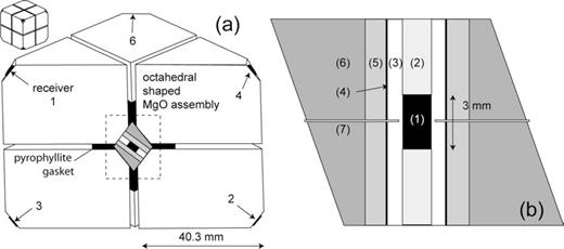
Multi-anvil sample assembly. (a) Cross-section of the assembly along the sample axis. The sample is located in the centre of the octahedral MgO cell. Adjacent anvils are separated by pyrophyllite gaskets. Arrows indicate positions of receivers. Receivers 1 and 2 are placed directly in line with the sample axis. Receivers 3–8 are placed at ±70.5° with the sample axis. (b) Detailed cross-section of the MgO cell: (1) sample, (2), steel buffer rods, (3) MgO sleeve, (4) Mo furnace, (5) ZrO₂ sleeve, (6) MgO octahedron and (7) thermocouple.

Open in new tabDownload slide

Although traditionally designed for hydrostatic purposes, multi-anvil assemblies can be used for deformation studies by placing additional ‘hard’ buffer rods at either end of the sample. The presence of the hard buffer rods generates a differential stress, with the maximum principal stress along the axis of the sample. This differential stress causes the sample to deform in axisymmetric compression and extension during pressurization and depressurization.

We note that it is not possible to measure the differential stress or strain history directly in our deformation experiments. The quantification of the stresses involved is a topic of future work, in which the AE-technique will be combined with synchrotron X-ray diffraction. In the current set-up, vertical compression rates are initially very fast, associated with high strain rate deformation (pressure cell shortens with 10⁻⁴ s⁻¹ during first 2 GPa) and high differential stresses. Such conditions will result in measurable AE, even up to pressures of 6 GPa at 900 °C.

As a proof-of-concept of the AE technique, we first tested the experimental set-up during six constant rate compression experiments on 8 mm long × 2 mm diameter polycrystalline corundum (Al₂O₃) samples. Two pre-cut notches were made on opposite sides of the sample in order to facilitate shear faulting in the sample during compression. We subsequently performed nine experiments during which we studied microseismicity associated with high-pressure deformation of dense (<2 per cent porosity), 3.0 mm long × 1.5 mm diameter San Carlos olivine samples. These samples were prepared by hot-pressing olivine powders (grain size: 200 (80 per cent) + 10 (20 per cent) μm) for 5 hr at 300 MPa and 900 °C, using a Paterson apparatus. In this paper we present results from two characteristic experiments that illustrate our principal findings.

2.2 Monitoring microseismicity

In our high pressure experiments, AEs associated with fracturing processes are detected by an array of piezo-electric transducers (microseismic receivers) that register the arrival of wave packets, or ‘hits’, at each receiver. We recorded and processed AE signals using the AMSY-5 high-speed multi-channel acquisition system from Vallen-Systeme GmbH. This system can record AE hits at a rate of 30 000 s⁻¹ and is additionally capable of recording a full waveform for each AE hit at a 10 MHz sampling rate (16 bit, 2048 samples). Received signals are amplified using programmable gain pre-amplifiers before being transmitted to the main recording system. The gain was set to 40 dB in the present experiments.

Each AE hit can be characterized by the recorder in terms of a number of user-chosen parameters; most importantly its trigger (‘first threshold crossing’) time, maximum amplitude (within a dynamic range of 0–100 dB) and energy (signal strength obtained by integrating the absolute amplitude value of the hit) (Fig. 2). We front-end filtered incoming data to reduce the amount of recorded noise from physical and electrical sources in the laboratory environment and, hence, to constrain the amount of data stored during each experimental run. AE signals and their waveforms were saved to disk when a predefined amplitude threshold of 44.9 dB (equivalent to 0.1 mV ‘threshold amplitude’) was crossed repeatedly for at least four times (Fig. 2). The waveform records are set to have a duration of 2048 samples (∼200 μs). These settings allowed full waveform recording (including a pre-trigger time of 40 μs) of all signals above the amplitude threshold while maintaining storage files at a manageable size of 2 GB of hard disk space.

Figure 2

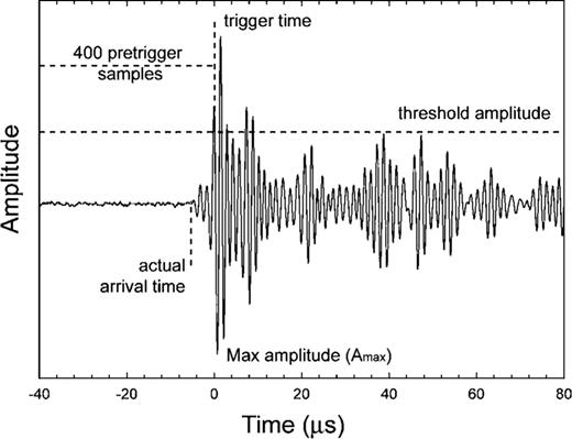
Sample waveform of a high frequency (830 kHz) acoustic emission during olivine deformation at 5.5 GPa pressure. The hit is recorded when the threshold amplitude is crossed more than four times. Note that the time of the first threshold crossing (trigger time) is not equal to the arrival time of the hit at the receiver.

Open in new tabDownload slide

2.2.1 Piezo-electric transducers

Microseismic events are collected at eight receivers that are attached to the back truncations of the eight tungsten carbide anvils (Fig. 3a). In order to generate enough space for the receivers inside the pressure vessel, special 28.5 mm edge-length carbide anvil cubes were manufactured (against the standard edge-length of 26 mm). Additional cable exits were also machined into the first-stage wedges and the pressure vessel cover (Figs 3b and c).

Figure 3

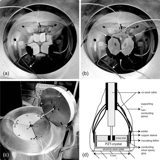
Receivers for AE monitoring in multi-anvil experiments. (a) Photograph of the 14/8 octahedral sample assembly on top of four anvils. Transducers are mounted on the back truncation of each tungsten carbide anvil. Note the cable of the bottom receiver (arrow). (b) Photograph of the entire assembly inside the pressure vessel. (c) Closed pressure vessel with exits for transducer cables. (d) Schematic cross-section of a transducer assembly. See text for details.

Open in new tabDownload slide

Each AE receiver consists of a 0.41 mm thick × 3.00 mm diameter piezo-electric crystal (lead zirconate titanate (PZT) with 150–1000 kHz bandwidth) suitable for detecting compressional P waves (Fig. 3b). Each transducer also has a 0.55 mm thick × 3.00 mm diameter brass backing plate. The advantage of PZT-based transducers over other materials, for example lithium niobate, is their high sensitivity, making them suitable to detect the low amplitude AE signals generated in small, millimetre-scale rock samples, even during high temperature experiments. Despite the 250 °C Curie temperature of PZT, our transducers were able to function efficiently during experiments at temperatures up to 1000 °C, because the transducer temperature at the back of the anvils never exceeded 150 °C.

An incoming longitudinal sound wave creates a strain pulse across the PZT crystal, which generates an electrical potential difference between the front and back face. A miniature co-axial cable is connected to the back face of the crystal through a 0.7 mm hole in the brass backing plate. The front face is connected to a 1.5 mm long × 3.96 mm diameter outer Cu-sleeve by glueing the PZT crystal and Cu-sleeve to an alumina wearplate with silver-doped epoxy. Two teflon insulators electrically isolate the back face of the PZT and the brass disk from the outer copper sleeve. The entire receiver assembly is potted in non-conductive epoxy resin to provide support and stability to the transducer during use. The transducer assemblies were coupled to the back truncations of the anvils with cyanoacrylate adhesive. Subsequent pulser tests confirmed that traveltimes from the front truncations of the anvils to the transducers were consistent to better than 0.05 μs.

2.2.2 Array size, traveltimes and velocity

During pressurization the sample assembly compacts significantly. As a consequence, the receiver array spacing decreases with increasing pressure. In order to calculate the change in receiver spacing with pressure, a calibration was made of axial shortening of the assembly as a function of confining pressure (Fig. 4). Most assembly compaction occurs in the initial 3 GPa, during which the MgO cell and the pyrophyllite gaskets are crushed and consequently configure into an essentially zero porosity solid pressure medium. Little compaction occurs at pressures above 4 GPa.

Figure 4

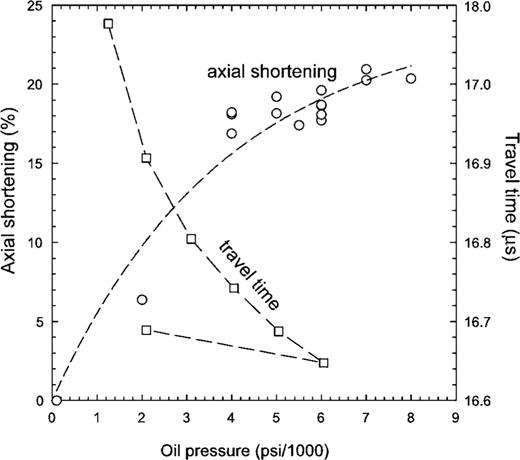
Assembly compaction with oil pressure. Left axis: circles indicate the axial shortening of the assembly along the sample axis. Most compaction occurs at oil pressures up to 3000 psi (∼3 GPa confining pressure). Right axis: squares indicate the change in P-wave traveltime with oil pressure for two opposing transducers directly above and below the sample during one complete cycle of compression and decompression. The traveltime decreases when the assembly compacts with increasing pressure. The assembly remains compacted during decompression.

Open in new tabDownload slide

P-wave traveltimes between pairs of opposite transducers (t_op) were calibrated at 1 GPa pressure intervals during each experiment, in order to determine average P-wave velocities (V_p) of the assembly at high pressure and temperature conditions. During calibration, each transducer is pulsed in turn to send bursts of high amplitude energy which are recorded at the remaining transducers. The arrival time detection of the pulses is very precise because the high amplitude and rapid rise of the pulsed waveforms are clearly distinguishable from background noise. Fig. 4 shows an example of how the traveltime can be monitored during an entire pressurization cycle. Average P-wave velocities (V_p) of the assembly can be estimated for the different compression, heating and decompression stages in an experiment because the dimensions of the tungsten carbide anvils are well known. We assume that the assembly can be treated as a homogeneous velocity medium. The assemblies have a V_p of approximately 6.1 ± 0.5 mm μs⁻¹ (∼V_p of tungsten carbide) and traveltimes between opposite receivers at high pressure is ∼16–17 μs (Fig. 4). The energy received at each transducer during this calibration serves as an effective measure of the quality of the coupling of the receiver to the anvil.

2.3 Hypocentre location

A first estimation of event locations is made using the Vallen Visual AE software. The program allows hits recorded successively at different transducers to be grouped into an AE event. This so-called ‘event builder’ takes into account the dimensions of the sensor array and a user-defined time difference that is allowed between successive hits within one event. We define this time to be 20 μs in the current assembly, which filters out most of the noise from the press without loosing signals from the assembly.

Over 50 000 events are recognized during a standard experiment. The problem is in deciding which events are associated with microcracking in the rock sample. One shortcoming of Vallen location data is that trigger times rather than true arrival times are used in the location algorithms (Fig. 2). The time difference between the trigger time and the true arrival time can vary by up to 25 μs. As a result, it is not possible to use this algorithm to locate AE sources at submillimetre accuracy, since this requires arrival time precision to be of the order of 0.1 μs. Therefore, in order to improve the location accuracy we used the standard data acquisition software to simply define the events of interest, and subsequently recalculated their locations using the much more rigorous procedure described below.

2.3.1 Arrival times

One possible estimate for arrival times can be obtained by means of a rise time correction. In the simplest case, the arrival time is considered to equal the linearly extrapolated time from the maximum amplitude and trigger time onto the waveform baseline, as applied by Dobson (2004). However, this correction is only approximate and, therefore, not adequate for our purpose.

Consequently, in order to better estimate the P-wave arrival time for each hit, we analysed the corresponding waveforms using the Akaike Information Criterion (AIC, after Akaike 1973). The AIC approach is based on the assumption that a seismogram can be divided into locally stationary segments in an autoregressive process. The intervals before and after the onset of the P wave are considered to be two different stationary processes (Sleeman & van Eck 1999). When applied directly to a seismogram x of length N, the AIC function is defined by Maeda (1985) as:

where k equals the number of samples in the seismogram. The arrival time, or onset of the waveform, is simply equal to the minimum value of the AIC function. The AIC technique has been applied successfully in other rock deformation studies (e.g. Zhang 2003) although there is a tendency for it to be less suitable when applied directly to unprocessed high frequency acoustic signals (Kurz 2005) or signals with low signal-to-noise ratios. We therefore focused on the locations of higher energy events with amplitudes above 60 dB, since these events also have a very short rise time, which tends to minimize the picking error.

2.3.2 Location algorithm

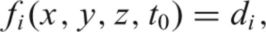
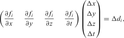
We calculated hypocentres for events with a minimum of five arrival times. The location algorithm used here assumes point source events and a straight source-to-receiver ray path. Hypocentres are, therefore, less well resolved outside the MgO cell, for example, in the pyrophyllite gaskets.

The arrival time observation of an AE event at a receiver can be written as a function of the source location [x, y, z] and the origin time t₀,

where d_i is the arrival time of the ith observation. The hypocentre source parameters x, y, z and origin time t₀ can be calculated using the classical method of Geiger (1912), which states that a perturbation of the source parameters and the resulting perturbation of the arrival times of acoustic waves are linearly related. In matrix form, the problem is described as

where Δd_i=d_i−f_i(x, y, z, t₀) is the arrival time residual, that is, the observed arrival time minus expected arrival time. The problem is solved using iteration and generalized least-squares inversion (Lay & Wallace 1995),

in which Δm= (Δx Δy Δz Δt₀)^T contains the perturbations in source parameters that need to be determined. G_ij is a matrix of size i×j (i is the number of hits per event, ranging from 5 to 8, j is the number of source parameters, which is 4) containing the partial derivatives that denote the effect on the ith observation of perturbing the source parameters. In order to take into account the a priori error in arrival time and the a priori error in the location, we applied the weighted iterative least-squares (WLS) method of Tarantola & Valette (1982). Using this method, we find location solutions that fit within the well-defined dimensions of the sample. Δm is again found using iteration, that is,

where C_d is a n×na priori data covariance matrix with arrival time errors (σ²_t) along its diagonal, C₀ is the a priori model covariance matrix, m_i is the vector [x  y  z  t₀] after each iteration and m₀ is the initial estimate of the hypocentre parameters. The initial value of m₀ is set to [0 0 0], that is, the centre of the sample assembly.

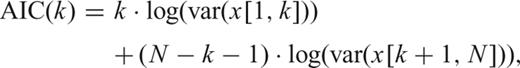
We set C₀ equal to the physical dimensions of the sample in the x, y and z directions. The error in arrival time, σ_t, is set to the mean time difference between automatically and manually picked arrival times of 500 randomly chosen waveforms. We determined σ_t for the compression, heating and decompression stages of each experiment. We chose not to apply an additional L-curve correction (e.g. Hansen 1992) to the WLS-method so that the location solution only takes empirical observations into account with no extra statistical damping. In addition, we have made a correction for the orientation and surface area of the transducers.

The a posteriori covariance matrix C_p gives a way to quantify the errors in the resulting models:

in which the diagonal elements of C_p represent the squared error of the model parameters x, y, z and t₀. The location error (σ_x, σ_y, σ_z in millimetres) in the [x y z] directions are typically of the order of [0.79 0.78 1.81] and [0.68 0.68 1.07] for corundum and olivine hypocentres, respectively.

In an attempt to elucidate more detailed structural features that may occur in the hypocentre clusters, we have tested the double difference technique of Waldhauser & Ellsworth (2000) as well as the joint hypocentre determination method of Douglas (1967). Neither routine improved the location errors or their spatial arrangement. We suspect that the required corrections on a millimetre scale are difficult to achieve at the high P-wave velocities around 6.6 mm μs⁻¹. The Matlab©-code of the location algorithms will be the subject of another paper.

2.4 Waveform analysis

In order to obtain information on the deformation mechanisms operating in the sample, we analysed the waveforms of each event for their polarity at the automatically picked AIC arrival time. For example, AE from compressional (or extensional) faulting are expected to result in negative (or positive) first motions of the two transducers directly above and below the sample (Fig. 1). The polarities of the first motions at the other receivers, which are at ±70.5° to the sample axis, depend on the location and orientation of the hypocentre. AE originating from pore collapse and compaction of the pressure medium are expected to have overall negative polarities, while AE from fault slip events are expected to show both positive and negative (double couple) polarities. Fig. 5 shows an example of an 8-hit event and the first motions of the arrivals at each receiver.

Figure 5

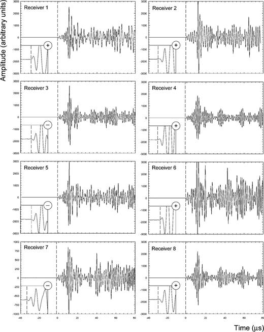
Waveforms of an 8-hit event during olivine decompression from 6 GPa. These high amplitude waveforms have little noise and a frequency range of ∼400–800 kHz. They are analysed using the AIC algorithm (Maeda 1985) to obtain the times of first arrivals (dashed lines) and their polarities (insets). Note the smaller amplitude scale of receiver 7.

Open in new tabDownload slide

We subsequently determined a composite focal mechanism solution for each experimental stage on the basis of the dominant polarity of hits received at each transducer during that stage. The focal mechanisms are plotted on an equal-area upper hemisphere projection, in which the sample long axis is parallel to the equatorial plane. In this way, the equatorial plane reflects a cross-section through the sample assembly so that it is possible to directly compare the mechanism to microstructures observed in the sections of recovered samples. The lower hemisphere stations are projected through the origin onto the upper hemisphere. The energy and amplitude data were not used in the focal mechanism because different coupling properties between different transducers and the attenuation properties of different materials in the experimental assembly have not currently been calibrated.

3 ILLUSTRATIVE RESULTS

3.1 Deformation of corundum

3.1.1 Event record

In order to validate the method, we first studied axisymmetric compression of polycrystalline corundum (Al₂O₃) rods up to 4 GPa at room temperature. Fig. 6 represents a typical record of AE events measured for the duration of an experiment. The record is characterized by an initial peak of AE activity up to about 0.5 GPa. These signals originate from the crushing and compaction of the MgO sample assembly as well as the pyrophyllite gaskets configuring themselves between the tungsten anvils. Comparison of the AE energy rate with the AE event rate illustrates that the assembly compaction is dominated by many low energy events.

Figure 6

Energy rate (top) and event rate (bottom) of AE from the cubical sample assembly, recorded during a corundum deformation experiment to 4 GPa, followed by decompression. A single event is defined by five or more hits. Energy scale in eu (1 eu = 1 × 10⁻¹⁴V² s) and time bin width is 32 s.

Open in new tabDownload slide

With increasing pressure, the experimental set-up becomes acoustically quieter as the assembly adjusts to a high pressure configuration. High-energy peaks up to 11 000 eu (1 eu = 1 × 10⁻¹⁴V² s) are observed upon further compression to 2 GPa, for example at t= 4000–6000 s (Fig. 6). In combination with a lower event rate, these energy peaks indicate that the axisymmetric compression is characterized by higher energy events that are possibly related to brittle deformation of the hard sample. Subsequent pressurization to 4 GPa is characterized by a low level of background noise with a sequence of high energy events.

The decompression stage of the experiments is very quiet. Most microseismicity occurs during the very last stages of decompression. This is caused by the sudden release of high pressure in the cell when retracting the hydraulic ram below oil pressures of 1000 psi (∼6.89 MPa), while the sample is still experiencing approximately 2 GPa of confining pressure.

3.1.2 Microstructure and hypocentres

Axisymmetric deformation of the corundum sample during compression primarily resulted in a well-defined axial fracture that runs parallel to the main compression direction (i.e. ‘mode I fracture’, Fig. 7a). Directly surrounding this fracture is a zone of fine-grained material, indicating significant internal crushing of the sample. Other fractures are found at the top of the sample and opposite the two pre-cut notches at the sample surface. None of our samples faulted along a plane between the pre-cut notches.

Figure 7

Deformation of corundum. (a) Reflected light micrograph of sample cross-section. The internal part of the sample is crushed, indicated by its light grey appearance. Brittle fractures (dashed lines) occur near the top of the sample and along its vertical axis. (b) 3D-view of the sample between four tungsten anvils, with hypocentres for events >60 dB during axial compression to 4 GPa. Hypocentre annotation: closed-large = inside the sample, closed-small = within 1σ from the sample, open-small = outside 1σ from the sample. (c–d) 2-D projection of the hypocentres on the sample cross-section in (a), for compression to (c) 0.5 GPa and (d) from 0.5 to 4.0 GPa. In both compression stages, hypocentre clusters dominantly locate near the central and top fractures and the light-coloured damage zone in (a). Parameters used in the location algorithm: V_p= 6.1 mm μs⁻¹, σ_t= 0.6 μs. The location error ellipsoid in [σ_x σ_y σ_z]=[0.79 0.78 1.81]. We note that >95 per cent of the events fall within 2σ from the sample.

Open in new tabDownload slide

3-D hypocentres of events with A_max > 60 dB were calculated for the compression and decompression stages of the experiment. During compression, 170 events were located in the sample (Fig. 7b). Most of these events occurred during compression to 0.5 GPa confining pressure. The event locations form clusters near the faulted sample top and appear to locate along the sample axis, within the light grey damage zone and along the mode I fracture (Fig. 7c). The high energy peaks during compression from 0.5 to 4 GPa correspond to events that dominantly locate on the vertical mode I fracture (Fig. 7d). More than 95 per cent of the located events fall within 2σ location error of the sample volume.

A relatively large time-error of σ_t= 0.6 μs in the location calculation is caused by the large amount of background noise from signals generated at low pressure. All transducers show dominantly negative arrivals, which is consistent with crushing of the sample. In this case, a focal mechanism is difficult to determine but reflects a uniform collapse of the sample during compression (Table 1). No events were located in the sample during the decompression stage, which is consistent with the lack of decompressional faults in the sample.

1

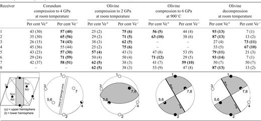
Polarity of waveforms per station for hypocentres located in the sample volume. The percentages of the first motions (positive = Ve⁺, negative = Ve⁻) are listed for the corundum and olivine hypocentres in Figs 7 and 9. Bracketed numbers denote the number of analysed waveforms per receiver. Percentages in bold indicate that |Ve⁺−Ve⁻ | ≥ 10 per cent. A possible composite focal mechanism solution in an equal-area upper hemisphere projection is given for each stage in the experiment. Symbols: Ve⁺= black, Ve⁻= white. The inset shows the position of the receivers in a hemisphere projection. Stations 1 and 2 lie along the sample axis and within the equatorial plane. Lower hemisphere stations are projected through the origin onto the upper hemisphere. We note that the interpretation of polarity at 900 °C is more difficult due to increased noise (see text).

Open in new tabDownload slide

In summary, we observe dominantly negative arrivals during pressurization, which corresponds to compressional deformation settings. The event hypocentres in the sample coincide well with microstructural observation in the sample, i.e. they correspond to an axial fracture along the sample long axis and its surrounding damage zone as well as some smaller fractures in the top of the sample.

3.2 Deformation of olivine

3.2.1 Event-record

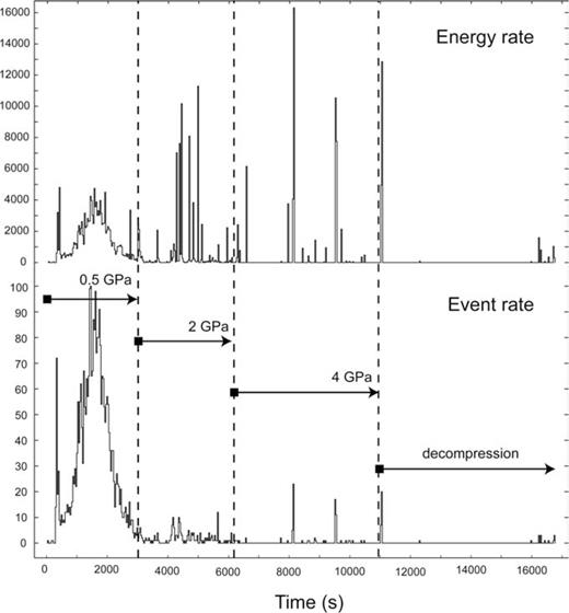
We have subsequently studied AEs associated with brittle deformation of olivine up to 6 GPa and 900 °C. Fig. 8 shows the event-rate and energy-rate during a typical olivine deformation experiment. Again, the AE record shows the dominance of assembly compaction during the early phase of pressurization. The event-rate then strongly declined when the assembly was compacted above ∼1 GPa. Between 1 and 2 GPa (interval t= 4000–10 000 s), the combination of high energy peaks up to 10 000 eu with low event rates (<100) suggests that the olivine sample undergoes brittle failure. Subsequent heating of the assembly to 900 °C at 2 GPa resulted in a very quiet period of thermal relaxation of the assembly. Hot compression to 6 GPa at 900 °C produced another period of AE activity with smaller high-energy peaks of around 1000 eu. Depressurization was quiet with only a few low-amplitude background events. However, a large burst of AE activity occurred at very low oil pressures.

Figure 8

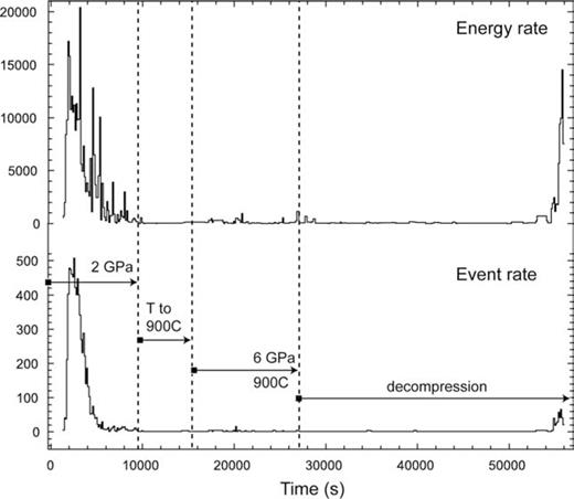
Energy rate (top) and event rate (bottom) of AE from the cubical sample assembly, recorded during an olivine deformation experiment. A single event is defined by 5 or more hits. The olivine sample was deformed during (1) compression to 2 GPa, (2) compression to 6 GPa at 900 °C and (3) decompression at room temperature. Energy scale in eu (1 eu = 1 × 10⁻¹⁴V² s) and time bin width is 128 s.

Open in new tabDownload slide

3.2.2 Microstructure and hypocentres

Axisymmetric compression of the olivine sample typically resulted in a fault system with a conical shape in three dimensions. In a 2-D sample cross-section, these conical faults are expressed a set of conjugate faults (Fig. 9a). The largest fault runs at 30° to the maximum compression direction (from the sample top right to bottom left in Fig. 9a). The fault displacement is clearly illustrated by the offset of two gold markers in the olivine sample. The AE-record suggests that the brittle failure of the sample occurred between 1 and 2 GPa because the largest energy events were generated in this pressure interval (Fig. 8). We were able to locate 8 high-amplitude events within the sample (A > 70 dB) during compression up to 2 GPa (Fig. 9b). These events appear to follow the orientation of the two main fault planes in the 2-D sample cross-section.

Figure 9

Deformation of olivine. (a) Reflected light micrograph of the deformed sample in cross-section. Brittle deformation of the olivine sample resulted in a conjugate set of faults (dashed lines). Fault displacement is indicated by gold markers (arrow). (b–d) 2-D projections of hypocentres for events >70 dB onto the sample cross-section in (a). Hypocentre annotation: closed-large = inside the sample, closed-small = inside the sample using location error range, open-small = outside the sample. (b) ‘cold’ axial compression of olivine to 2 GPa is marked by hypocentres near the large conjugate fault set. (c) Hypocentres are more dispersed at the top of the sample during ‘hot’ compression to 6 GPa at 900 °C. The inset (view perpendicular to (c)) shows location clusters outside the sample. (d) Events during ‘cold’ decompression from 6 GPa locate near the large sample faults again. Parameters used in the location algorithm: (a) V_p= 5.7, mm μs⁻¹, σ_t= 0.5 μs, error ellipsoid =[0.69 0.69 1.10], (b) V_p= 6.25 mm μs⁻¹, σ_t= 0.8 μs, error ellipsoid =[0.77 0.79 1.40], (c) V_p= 6.6 mm μs⁻¹, σ_t= 0.2 μs, error ellipsoid =[0.58 0.57 0.72].

Open in new tabDownload slide

During cold compression of olivine, negative first motions are measured above and below the sample at receiver 1 and 2, as well as laterally at receiver 3 and 4 (Table 1). Receivers 5, 7 and 8 have dominantly positive arrivals. The focal mechanism that fits these polarities consists of a fault plane dipping 30° into the equatorial plane (i.e. into the sample cross-section in Fig. 9a). This fault plane represents a 90° rotation of the top-right-to-bottom-left fault in the olivine sample cross-section along the conical fault surface (i.e. perpendicular to the section in Fig. 9a). Despite the relatively low number of located events, the waveform polarity indicates a displacement that is consistent with a maximum stress in the axial direction.

We measured different values for the arrival time error σ_t during the ‘cold’ compression (σ_t= 0.5), ‘hot’ compression (σ_t= 0.8) and ‘cold’ decompression (σ_t= 0.2) stages of the experiment. A σ_t of 0.8 μs during compression to 6 GPa at 900 °C might have been caused by electrical noise associated with the furnace. P-wave velocities were substantially higher (V_p > 6.2 mm μs⁻¹) at 2–6 GPa and 900 °C than at P < 2 GPa (V_p∼ 5.7 mm μs⁻¹) (Fig. 9).

Hypocentre determination at 900 °C was difficult because the wiring of receiver 3 and 4 malfunctioned in this particular experiment, limiting the location calculation to a maximum of 6 hits per event. We found two main clusters of hypocentres, one outside and one inside the sample volume, which are potentially associated with high pressure frictional sliding on the pre-existing faults (Fig. 9c). The polarity of events located inside the sample (Table 1) fit well to a focal mechanism that is based on the ‘top-left-to-bottom-right’ conjugate fault in the 2-D sample cross-section (Fig. 9a). It is observed that receivers 1 and 2 have a reversed polarity compared to events generated during cold compression, which implies an unlikely axisymmetric extension of the sample (‘backslip’) on the pre-existing conical faults during pressurization. Closer examination of the waveforms suggests that these polarities are more difficult to determine at high temperature because of the higher amplitude of noise at 900 °C (Fig. 9c). High amplitude noise can cause the AIC-algorithm to pick the actual arrival time at systematic time offset of half a wavelength of the AE frequency (e.g. ∼0.6 μs at 830 kHz, Fig. 9c). The polarity of located events is, therefore, possibly reversed, which would explain the observed polarity reversal during compression at temperature.

The high energy peaks and increase in event rate during the decompression stage are associated with several events in the olivine sample, which locate very close to the trace of the conical faults on the 2-D sample cross-section (Fig. 9d). It is expected that the sample extends axially during decompression, and extension should result in positive arrivals at the sample ends, that is, receiver 1 and 2, and negative arrivals at receiver 3 and 4, which is indeed the case. Axisymmetric extension of the sample during depressurization along the ‘top-left-bottom-right’ conjugate fault trace in the 2-D sample cross-section is consistent with positive arrivals at receiver 1, 2, 5, 6 and 8 and negative arrivals at receiver 3 and 4 (Fig. 9a, Table 1).

4 DISCUSSION

Summarizing the results, the proof-of-concept experiments on corundum and olivine demonstrate that it is possible to locate the hypocentres in millimetre scale samples using an 8-transducer system and by including an a posteriori estimate of the uncertainty in the arrival time measurements. The comparison of potential hypocentre locations to the brittle deformation microstructures observed in the recovered samples shows that events can be satisfactorily located near faults in the sample. More importantly, composite focal mechanisms that are based on the P-wave polarity of located sample events are in good agreement with fault orientations in the recovered samples as well as the deformation regimes in the experiment (i.e. compression and extension stages). Therefore, the new 8-transducer AE setup for high-pressure multi-anvil experiments presented here enables us to successfully link high energy AE events to high pressure rock deformation during both axisymmetric compression and extension. Hence, this new AE-technique is an important addition to previous high-pressure AE studies.

4.1 Previous studies

Previous studies of AE in multi-anvil experiments reported by Dobson (2002, 2004) and Jung (2006) were able to link AE hypocentres to dehydration reactions in serpentinite at high pressure. It was suggested that acoustic signals were associated with sample deformation when the time difference of arrivals within an event was less than the travel time across the sample. The current set-up improves these previous studies because it allows us to perform more accurate 3-D hypocentre location in the multi-anvil assembly, which in turn can be compared to waveform analysis and rock deformation microstructures.

The current experimental set-up is somewhat different from the 4-transducer system of Jung (2006). First of all, they used lithium-niobate transducers. Lithium-niobate transducers are ideally suited to experiments under high-temperature conditions because of their high Curie temperature. However, their use may also lead to a reduction in the AE detection because lithium-niobate has a relatively low piezo-electric coefficient, making it insensitive to low amplitude signals. Secondly, we chose to use a metal foil furnace with low P-wave attenuation, which facilitates accurate detection of AE signals that radiate normal to the sample axis. In addition, the large redundancy introduced by using 8 transducers allowed us to use much lower threshold values (0.1 mV compared to 100 mV of Jung 2006) and increase the amount of collected data. The calibrations of arrival time differences between opposite receivers at varying pressures imply that the maximum arrival time difference across the rock specimen is ∼0.5 μs in the present set-up, which is a much lower value then previously reported for set-ups with fewer transducers (Jung 2006).

4.2 Hypocentre location

Locating the hypocentres in the small scale structures of the rock specimens is not straightforward and is influenced by a number of factors. Here we discuss the main ones.

(1) Number of receivers

It is a rule of thumb that the accuracy of hypocentre location increases with the number of hits on receivers per event. The hypocentres presented in Figs 7 and 9 dominantly comprise events of 6–8 hits. Our results were only possible by extending the existing AE set-up for multi-anvil experiments to an 8-receiver system. At present, eight receivers is the maximum that can be achieved in standard double-stage Kawai-type multi-anvil press designs.

(2) Signal-to-noise (S/N) ratio of the waveforms

The total error in a location is primarily a combination of measurement error and the velocity model (Pavlis 1986). The measurement error, that is, the arrival time, is influenced by (1) noise in the cell (other extraneous events) and (2) the sampling rate of the waveforms. Therefore, the quality of the recorded waveforms plays an important role in finding the correct hypocentre location.

It is likely that many potential sample hypocentres were located incorrectly due to inaccurate arrival times of one or more hits within the event. Inaccurate data will easily cause the hypocentre location algorithm to iterate away from the source. This might explain why relatively few events were located in the low-pressure stage of the olivine experiment (Fig. 9), where a high level of noise (due to assembly compaction) might have influenced the event building process. Furthermore, excluding arrivals with noisy waveforms may result in a bias of the hypocentre solution towards certain directions because of the highly symmetric geometry of the receiver array. The AE clusters outside the olivine sample at 900 °C (Fig. 9c) may reflect the problem that two receivers malfunctioned.

Fortunately, hypocentre determination during decompression involves small time errors (σ_t= 0.2). When the assembly is compacted at high pressure, waveforms have high S/N ratios and fewer background events take place. Therefore, accurate hypocentre determination is possible in the relevant high pressure range of deep-focus earthquakes. In the case of high temperature experiments, it is important to reduce high amplitude noise from the experiments, as it has a clear effect on the AIC arrival times and polarity interpretation (Fig. 10). The increased noise during heating is likely to be due to electrical noise on the heating circuit. This can be effectively eliminated by replacing the present phase-angle firing thyristor control (which truncates the waveform of the AC heating current) with an amplitude modulated heating control system.

Figure 10

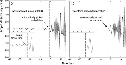
Characteristic example of the effect of noise on waveform arrival times and polarity. At 6 GPa pressure, waveforms recorded and 900 °C (a) have higher amplitude noise than those at room temperature (b). As a result, the arrival times determined with the AIC algorithm can differ from the actual arrival time, typically up to ∼0.6 μs. This time difference roughly corresponds to half a wavelength of a ∼830 kHz acoustic emission (Fig. 2), and is associated with a polarity reversal. Waveform polarity is there more difficult to determine at 900 °C. The amplitude scale is identical in both plots.

Open in new tabDownload slide

(3) Time and velocity precision

The precision in time that is required to locate AE in the sample has to be of the order of 0.1 μs. Our applied waveform sampling rate of 10 MHz is just sufficient to obtain accurate arrival time data. This type of study may, therefore, benefit from a waveform sampling rate above 10 MHz or subsample cross-correlation techniques. In the hypocentre determination, we assumed the multi-anvil assembly to be a homogeneous velocity medium. It is observed however, that the location error in the z-direction is larger than in the x–y directions. This may reflect a difference in transfer function from the source to receivers 1 and 2 along the z-axis (e.g. along the long axis of the sample and buffer rods) with respect to receivers 3–8 (e.g. approximately perpendicular to the long axis of the sample and buffer rods). We are currently in the process of extending our location algorithms to include a more precise velocity model of the assembly that takes its different component parts into account.

(4) Location model

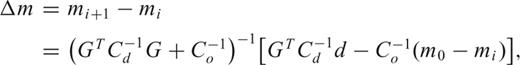
The location solution of the applied weighted iterative least-squares method strongly depended on the initial starting location m₀. It was observed that individual location solutions converge to the same spatial arrangements around the chosen m₀. This is a result of the imposed location model parameters (i.e. C₀ and C_d), which prescribe how a solution can vary within the applied time errors. It appears that the location solution is highly non-unique and that different choices of m₀ lead to different results. Because we are only interested in hypocentres from the sample volume, it is most straightforward and plausible to choose m₀=[0 0 0], that is, at the centre of the sample assembly, so that the reference model gives the best-fit event location with respect to sample centre. The accuracy of AE locations using the presented location algorithm might be improved significantly using the time difference of arrivals from cross-correlation techniques.

5 APPLICABILITY

AE monitoring during rock deformation experiments has been applied extensively before to study brittle failure and frictional sliding of rocks and the origin and characteristics of crustal earthquakes at upper crustal pressures (e.g. Lockner 1991; Sammonds 1992; Zang 1998; Lei 2000). The technique presented here improves on similar studies at ultra-high pressure (Dobson 2004; Jung 2006). We have demonstrated that it is possible to determine whether microseismic events originate from the sample. By combining waveform analysis with microstructural investigation of recovered sample, the technique is successful in determining the mode of cracking and in making first order estimations of focal mechanisms. These capabilities significantly extend the utility of laboratory studies aimed at unravelling the fault mechanisms of deep-focus earthquakes that occur during subduction at depths up to 650 km. We are currently developing this technique in combination with in situ X-ray diffraction to achieve estimates of the stresses required for faulting under the pressure and temperature conditions of deep-focus earthquakes.

It is generally accepted that deep-focus earthquakes are associated with high pressure phase transformations of olivine to wadsleyite and ringwoodite. Dobson (2004) demonstrated that the olivine-wadsleyite phase transition is clearly marked by periods of AE activity in multi-anvil experiments. We are currently extending our new technique to be applied to these higher pressures. An additional proof-of-concept study on a high-pressure chlorite transformation has recently been completed (Dobson 2007). Promising initial results demonstrate that the 8-transducer system is sensitive enough to detect and locate microseismicity associated with small-scale phase transformations that are caused by c-axis collapse of type-I clinochlore around 6 GPa (Welch & Crichton 2005). Future experiments at mantle transition-zone pressures will be applicable to the triggering of deep seismicity, elucidating details of seismogenesis and fault generation under the conditions of the subducting slab.

ACKNOWLEDGMENTS

Almar de Ronde is supported by a NERC research grant NE/C510308/1. David Dobson gratefully acknowledges the Royal Society for his Research Fellowship. This manuscript benefited from the constructive comments of two anonymous reviewers. We are very grateful to Arwen Deuss and Frederik Simons for extensive discussions and help on hypocentre algorithms and waveform analysis.

REFERENCES