Reducing the bias of multitaper spectrum estimates Free

Summary

1 INTRODUCTION

There are many applications in geophysics where relevant information contained in a given signal may be extracted from its power spectrum. In normal mode seismology (Gilbert 1970) and climate time-series analysis (Chappellaz 1990) the scientist may be interested in periodic components usually immersed in some background noise. A continuous spectrum is estimated from a short time-series in earthquake source physics studies (Brune 1970) and from bathymetry profiles to investigate seafloor roughness (Goff & Jordan 1988). The cross-spectrum is used to compare two signals in seismology (Vernon 1991; Hough & Field 1996), investigate the transfer function in electromagnetism (Constable & Constable 2004), and study the elastic thickness of the lithosphere (Simons 2000). In each of these cases, it is desirable to be able to obtain a reasonable spectrum, with little or no bias and small uncertainties. We present a brief review of some terminology, although the reader should have some familiarity with modern methods of spectral estimation; for more thorough theory and discussion see Percival & Walden (1993).

The periodogram (Schuster 1898) was the first (non-parametric) direct spectral estimate of the power spectral density (PSD) function. The periodogram is a biased estimate due to spectral leakage, the tendency for power from strong peaks to spread into neighbouring frequency intervals of lower power. It thus becomes necessary to use the method of tapering to effectively reduce this bias (Priestley 1981; Percival & Walden 1993).

For a data sequence x(t) with N points, the direct spectrum estimate at frequency f is:

1

where a(t) is a series of weights called a taper. Eq. (1) is sometimes called a single-taper, modified or windowed periodogram. If a(t) is a boxcar function, eq. (1) is called the periodogram.

In Thomson (1982) the multitaper spectral analysis method was introduced. In this method the data sequence x(t) is multiplied by a set of orthogonal sequences (tapers) to form a number of single taper periodograms, which are then averaged as an estimate of the PSD. This approach was introduced as an alternative to averaging in the frequency domain (e.g. smoothed periodogram) as a procedure to reduce the variance of the estimate. The multitaper method has been widely used in geophysical applications and has been shown in multiple cases to outperform the single-tapered, smoothed periodogram (Park 1987b; Bronez 1992; Riedel 1993). In the latter, a multitaper estimate that is subsequently smoothed is preferred.

Single taper estimates have a major limitation, in the sense that by using one taper a significant portion of the signal is discarded. The data points at the extremes are down-weighted, causing the variance of the direct spectral estimate to be greater than that of the periodogram. In the multitaper method, the statistical information discarded by one taper is partially recovered by the others. The tapers are constructed to optimize resistance to spectral leakage. The multitaper spectrum is constructed by a weighted sum of these single tapered periodograms. The weighting function is defined to generate a smooth estimate with less variance than single taper methods and at the same time to have reduced bias from spectral leakage.

The adaptive weighting proposed by Thomson (1982) is ideal to minimize spectral leakage but suffers from local bias. To achieve maximum suppression of random variability, the multitaper method must average the true spectrum over a designated frequency interval, introducing this second form of bias, which flattens out the local structure of the spectrum on the interval.

Riedel & Sidorenko (1995) suggested a different weighting function to minimize the local bias. They take a different set of orthogonal tapers and, assuming quadratic structure of the spectrum, reduce the bias introduced by the curvature of the spectrum. Because the chosen tapers minimize local bias, there is little spectral leakage reduction and this method does not perform as well with very high dynamic range signals.

In this paper, we present an improved multitaper spectral estimate using Thomson's method modified to reduce curvature bias. The second derivative of the spectrum is estimated by means of an expansion of the spectrum via the Chebyshev polynomials. Because we use the Slepian tapers and the adaptive weighting functions, the estimate is resistant to spectral leakage, yet reduces bias due to spectral curvature. In addition, we can estimate the derivative of the spectrum (slope), which can be used in parameter estimation or as a discriminant for comparing different signals.

This paper is organized as follows. In the next section, we outline the problem associated with the estimation of the PSD. After this, we provide a brief review of the multitaper spectrum estimation method and discuss some of its properties. Then, we introduce the new methodology, first explaining in Section 4 the estimation of the derivatives of the spectrum and in Section 5 the estimation of the unbiased spectral estimate. Finally, we give a number of examples to compare the original and the new multitaper methods. There is an application to bathymetric data and the application of the derivatives of the spectrum for comparing signals.

2 SPECTRUM ESTIMATION

In time-series analysis it is often useful to describe the PSD of the signal, given that it may have information of the background noise, periodic components, and transients. These pieces of information are fundamental in geophysics (Thomson 1990). For a more complete understanding of this section we point the reader to Priestley (1981), Percival & Walden (1993) and references therein.

To start (see Table 1), we need to consider a stationary stochastic process x(t), a zero mean discrete time-series consisting of N contiguous samples and assume that the sampling rate is always unity, so that t= 0, 1, 2, …, N− 1. Define the Fourier transform of the observations

2

We assume the signal is a harmonizable process, thus has a Cramér spectral representation (Cramér 1940)

3

for all t, where dZ(·) is an orthogonal incremental process (Doob 1952; Priestley 1981).

1

Essential notation and mathematical symbols used in this paper. In the text, means estimate of the variable θ; E[·] is the expected value and * represents the complex conjugate.

Open in new tabDownload slide

The random orthogonal measure dZ(f) has its first moment

4

and second moment (of relevance for our purposes)

5

where S(f) is defined as the PSD function of the process and E[·] is the expected value. Note here that the frequency variable f is continuous and so we are in fact trying to find a function S(f) from the finite series x(t).

Plugging the Cramér spectral representation (3) into the discrete Fourier transform (2), we arrive at the basic integral equation (Thomson 1982, 1990)

6

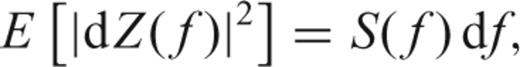
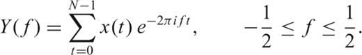
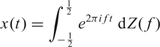
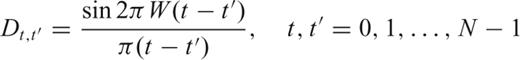
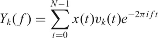
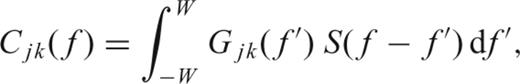
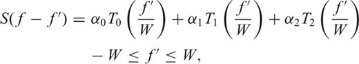
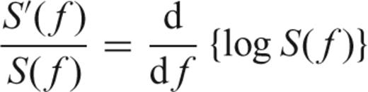
where is a modified Dirichlet kernel (see Thomson 1990; Percival & Walden 1993, eq. A11). The basic integral equation is a convolution that can be interpreted as the smearing of the true dZ(f) projected into Y(f), due to the finite duration of the time-series x(t).

This paper is about obtaining an approximate solution to this equation and based on that solution (via eq. 5) obtaining reliable estimates of the PSD of the signal.

3 MULTITAPER SPECTRUM ESTIMATES

We give a brief review of the standard theory for multitaper spectral analysis. Proof of various assertions can be found in (Thomson 1982, 1990; Park 1987b; Percival & Walden 1993). Note that given the properties of (6) and the smoothing of the Dirichlet kernel there is no unique solution to this problem. The multitaper spectrum estimate is an approximate least-squares solution to eq. (6) using an eigenfunction expansion. The choice of this type of solution will be explained next.

Choosing the windowed periodogram (eq. 1) as a spectral estimator is a natural first choice. Slightly rewriting the discrete Fourier transform (2) and squaring

7

where the sequence a(t) is called a taper. In the case of (2) the taper a(t) = 1 is a boxcar function. To maintain total power correctly a(t) needs to be normalized:

8

In the frequency domain, the properties of the taper are deduced from its Fourier transform

9

We call the function A(f) the spectral window associated with a. For conventional tapers, |A(f)| has a broad main lobe and a succession of smaller sidelobes (see Fig. 1).

Figure 1

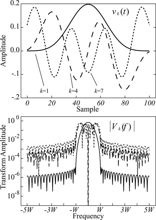
Selected Slepian sequences and corresponding Slepian functions for N= 100 samples and a choice of NW= 4. Sometimes called 4π Slepian sequences.

Open in new tabDownload slide

The choice of the taper can have a significant effect on the resultant spectrum estimate. One can observe this by expressing eq. (7) as a convolution of the transform of the taper (9) and the true spectrum

10

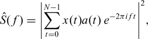
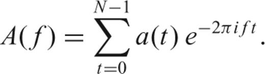
Here, as in (6), there is smearing or smoothing of the true spectrum. This means that the choice of window is important. A good taper will have a spectral window with low amplitudes whenever |f−f′| is large, leading to an estimate based primarily on information close to the frequency f of interest. The objective of the taper a(t) is to prevent energy at distant frequencies from biasing the estimate at the frequency of interest. This bias is known as spectral leakage. We wish to minimize the leakage at frequency f from frequencies f′≠f.

In practice, it is not sensible to be concerned about |f′−f| ≤ 1/N, since this is the lowest frequency accessible from a record of length N. A resolution bandwidth W is chosen, where 1/N < W≤ 1/2, and the fraction of energy of A in the interval (−W, W) is given by:

11

where λ is a measure of spectral concentration. It is clear that no choice of W can make λ greater than unity. Our task is to maximize λ.

To maximize λ substitute (9) in (11), take the gradient of λ with respect to the vector a=[a(0), a(1), …, a(N− 1)] and set to zero to obtain a matrix eigenvalue problem:

12

where the matrix D has components

13

and is symmetric.

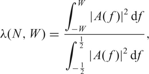
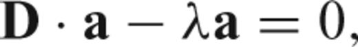
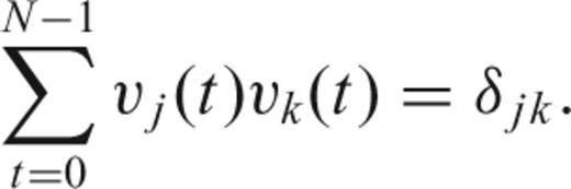
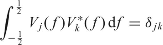
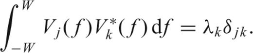
The solution of (12) has (dropping dependence on N and W) eigenvalues 1 > λ₀ > λ₁ > ⋯ > λ_N−1 > 0 and associated eigenvectors v_k(t), called the Slepian sequences (Slepian 1978). The first eigenvalue λ₀ is extraordinarily close to unity, thus making the choice a(t) =v₀(t) the taper with the best possible suppression of spectral leakage for the particular choice of bandwidth W. In fact, the first 2NW− 1 eigenvalues are also very close to one, leading to a family of very good tapers for bias reduction. The multitaper method exploits the fact that a number of tapers have good spectral leakage reduction, and uses all of them rather than only one.

3.1 Properties of Slepian sequences and functions

The Slepian sequences are solutions of the symmetric matrix eigenvalue problem (12)–(13). The eigenvectors with associated eigenvalues λ_k are real and orthonormal as usual

14

These vectors will be used as tapers in (7). We define the Slepian functions as the spectral windows, the Fourier transforms of the sequences

15

Note that the V_k's are complex functions of frequency. Fig. 1 shows three Slepian sequences and their corresponding Slepian functions.

One of the central features of the Slepian sequences is that orthogonality conditions also hold in the frequency domain (both in the whole and inner intervals),

16

17

It is convenient to define an orthonormal version of the V_k's on the inner interval (−W, W)

18

with the obvious property

19

This last property will be exploited in the sections to come. Fig. 2 shows a selection of the functions in the inner interval. Note how the real part of the functions is always even and the imaginary part is odd. See also how the amplitude of the functions increases outward as the Slepian function index increases and are more sensitive to structure further from the centre frequency.

Figure 2

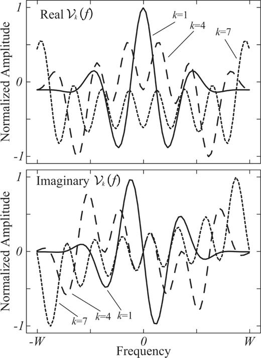
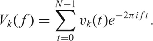
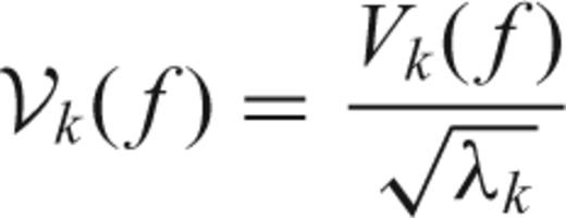
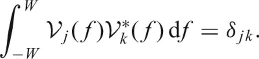
Orthonormal version of the Slepian functions in Fig. 1, in the inner interval. Only three functions are shown in the example with their real and imaginary amplitudes normalized. Number and thin lines show the index of the corresponding Slepian function plotted. The symmetry and amplitude of the functions are of interest.

Open in new tabDownload slide

3.2 The multitaper method

The objective of this method is to estimate the spectrum S(f) by using K of the Slepian sequences to obtain the keigencomponents:

20

and a set of K eigenspectra as in (7):

21

from which we can form the mean spectrum

22

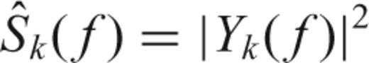
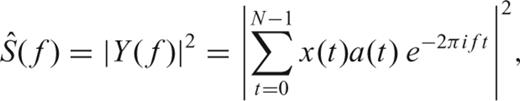
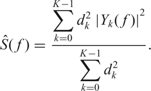
The idea of taking an average is to reduce the variance in the spectral estimate. As will be shown below, the mean spectrum is not an ideal estimate and we prefer a weighted average instead, one that minimizes some measure of discrepancy. While the spectral leakage properties of the eigenspectrum are very good, since the eigenvalues are close to unity when K < 2NW− 1, the leakage characteristics of the successive estimates degrade. It is clear that by using , the least amount of spectral leakage is achieved. Nevertheless, including the other eigencomponents (Y₁, Y₂, …, Y_K), while increasing spectral leakage, reduces the variance of the spectral estimate and is thus preferred.

In order to estimate the discrepancy of the different eigencomponents Y_k, we combine (20) with (3)

and using the definition of the Fourier transform of the taper (15) we obtain:

23

containing information from the whole interval ().

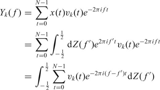
If the sequence x(t) were passed by a perfect bandpass filter from f−W to f+W before truncation to the sample size with N data points, we would obtain the idealized eigencomponents that, though unobservable, would be represented by:

24

Note that here we adopt the orthonormal functions , in order to maintain the correct normalization. The takes only information over the inner interval (−W, W).

In order to estimate , we find a set of frequency dependent weights d_k(f), as proposed by (Thomson 1982, 1990):

25

where σ² is the variance of the signal x(t). The multitaper spectrum is then obtained

26

Since we don't know the spectrum S(f) in (25), we are required to assume an initial estimate of the spectrum (averaging the first two k eigenspectra S₀+S₁ for example) and find the adaptive weights d_k iteratively. In (Prieto 2007) the reader can find a more complete discussion of the adaptive weights and a derivation can be found in Thomson (1982) or Percival & Walden (1993).

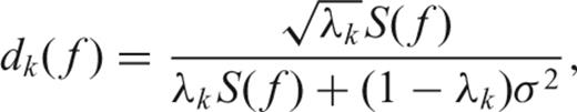
4 ESTIMATING THE DERIVATIVES OF THE SPECTRUM

At this point we introduce the covariance matrix of the multitaper components by an approach developed by Thomson (1990) which we will call the Quadratic multitaper method. More information about the spectrum can be obtained by looking at the covariance matrix of the K components at the single frequency f:

27

with j, k= 1, …, K. We use the orthogonal increment property (5) and substituting (24):

28

where . If the spectrum does not vary in the interval (−W, W) then the covariance matrix is diagonal

29

where I is the K×K identity matrix. Note that the multitaper spectrum in (26) is equivalent to taking the trace of C (f) and normalizing by the weights.

When the spectrum is constant in the interval (−W, W), the original multitaper method as proposed by Thomson (1982) is unbiased and provides an appropriate estimate of the spectrum. If, however, the spectrum varies within the interval, the matrix C(f) will not be diagonal and (26) may be biased. Clearly, we rarely obtain perfectly diagonal covariance matrices and the spectrum is not perfectly resolved.

Like (6)eq. (28) is a Fredholm integral of the first kind and suffers from similar non-uniqueness and smearing features, except in this case we have reduced spectral leakage and are only concerned about the interval (−W, W).

Thomson (1990) suggested taking a set of orthogonal eigenfunctions to expand the spectrum to solve (28). Here we propose to employ the Chebyshev polynomials for estimating the derivatives of the spectrum and using these derivatives to obtain an improved solution of the spectrum S(f). We prefer the Chebyshev polynomials (Mason & Handscomb 2003) because, as can be seen from Fig. 3, these polynomials are sensitive to structure at the edges of the interval, where the eigenfunctions proposed by Thomson (1990) have very little energy.

Figure 3

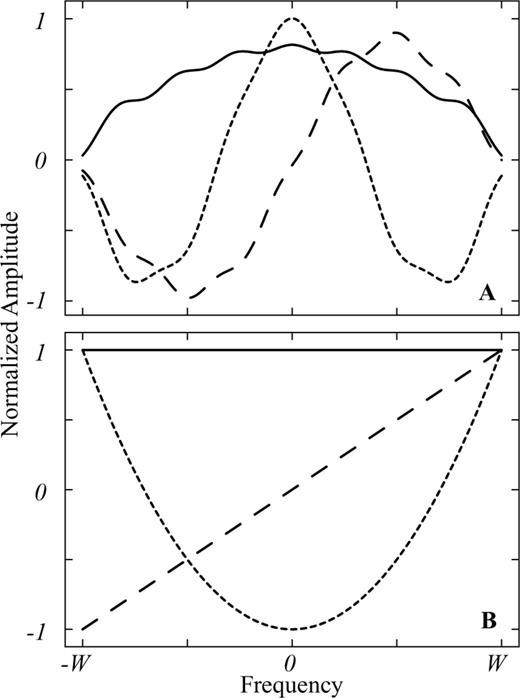
Comparison between first three basis functions used in Thomson (1990) (A) and Chebyshev polynomials (B) used in this study. Note that in (A), the basis functions always tend to zero when getting close to either −W or W and are not sensitive to structure at the boundaries. The Chebyshev polynomials in (B) are also very simple approximations of a constant, slope and quadratic terms.

Open in new tabDownload slide

We write the spectrum in the inner interval as:

30

where T_n(x) is the Chebyshev polynomial (Mason & Handscomb 2003) of degree n (see Fig. 3). Returning to the inverse problem (28) in spectrum estimation and inserting (30):

31

where the matrices

describe the zero, first and second derivative basis matrices. We can then obtain the Chebyshev coefficients, α₀, α₁, α₂, by solving the least-squares problem where we use the observed values of d_jd_kY_jY*_k to approximate the left-hand side.

The Chebyshev coefficients are estimates of the derivatives of the spectrum

around the centre frequency on the interval (f−W, f+W).

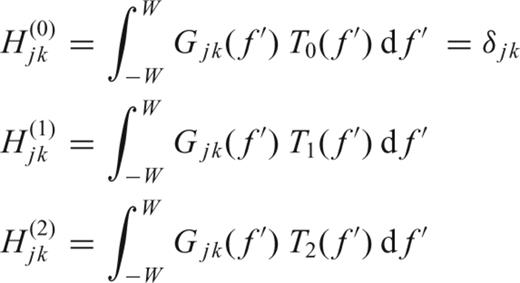
In practice, the calculation of the integrals in H⁽¹⁾_jk and H⁽²⁾_jk is done numerically using a trapezoidal quadrature. In Fig. 4, we plot the case of the three matrices in (31). The absolute values are plotted. Note that both the zero and second order terms are only present in the real part of the covariance matrix, while the first order term is present only in the imaginary part of the covariance matrix.

Figure 4

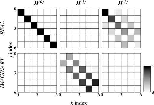
Comparison between the different basis matrices for zero (left-hand panel), first (middle panel) and second (right-hand panel) order coefficients. The absolute values are shown for simplicity. Note that the completely white matrices show that the real part of the covariance matrix is insensitive to slopes, while the imaginary part is insensitive to a constant and quadratic structure of the spectrum.

Open in new tabDownload slide

It is clear that the constant term will result in a diagonal covariance matrix, while the effects of the first and second order terms are quite different. H⁽¹⁾_jk has no effect on the diagonal terms, suggesting that this term does not bias the spectrum estimate (26). In contrast, H⁽²⁾_jk has an important contribution to the diagonal but is also present in the off-diagonal terms, showing the dependence of the eigencomponents in spectra that are highly variable. A slight correlation between the estimates of α₀ and α₂ is present.

5 REDUCING THE BIAS OF MULTITAPER ESTIMATES

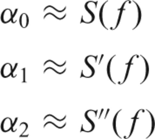
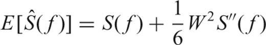
Up to now, the literature (e.g. Thomson 1982; Park 1992; Percival & Walden 1993, and many others) has assumed the spectrum varies slowly in this interval and can be taken out of the integral in eq. (28). Now, within (−W, W) we can try to find further information on the structure of the spectrum and relax the assumption of a constant spectrum inside the interval.

Assume the spectrum has a Taylor series expansion on the interval (f−W, f+W) of the form:

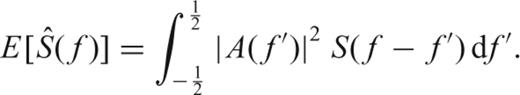
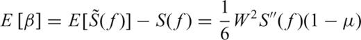
We know that the estimate of the spectrum at any frequency f is an average over the interval (f−W, f+W):

where the term associated with the first derivative does not contribute to the integral due to symmetry. Note that in Fig. 4 the matrix H⁽¹⁾, associated with the slope, is zero in the main diagonal and does not bias .

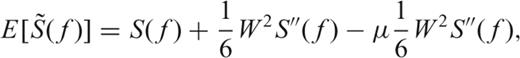
We can obtain the Quadratic multitaper estimate of the spectrum at frequency f by applying the correction:

32

where we assume obtained by solving (31). Note that we apply the correction to the multitaper estimate in (26).

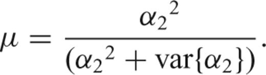
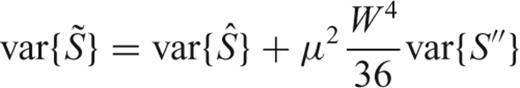
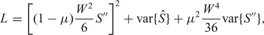
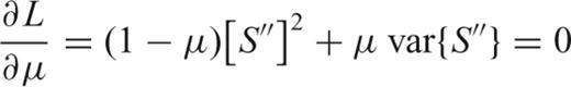
Applying the quadratic correction in (32) will increase the variance of the overall estimate, because is also uncertain. We propose to implement a mean-square error criteria instead of directly applying (32) to avoid exacerbating the uncertainties of the Quadratic multitaper:

33

where μ is a weight:

34

In Appendix A the derivation of the weight μ in (34) is explained as well as the approximate estimation of the variance of α₂.

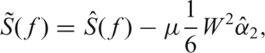
The Quadratic multitaper is an approximately unbiased estimate of the PSD of the signal analysed. As will be demonstrated in the next section with different examples, the Quadratic multitaper method provides a reduction of curvature bias while at the same time generating smooth estimates.

6 EXAMPLES

As a demonstration of the benefits of the Quadratic multitaper spectrum method (QMT) we show a number of synthetic examples and compare the results to the original (OMT) adaptive multitaper method by Thomson (1982). The main features we would like to concentrate on are the resolution close to significant structure in the spectrum, smoothness of the resultant estimates and the overall spectral leakage properties.

6.1 Random signal

The first signal to be analysed is a simple pseudo-random number r(t) with a normal distribution and standard deviation σ= 1. The number of data points for this example is N= 1000, For all plots in this paper we compute six tapers (K= 6) with 3.5 as the time-bandwidth product.

A visual inspection of the results of the two different methods in Fig. 5 shows that the method presented here generates a smoother spectrum than the original method. A more quantitative comparison is provided in Table 2, where 10 random realizations of a 1000 sample long random time-series were analysed and two different measures were used to assess the smoothness of the resultant spectrum: the norm of the second (numerical) derivative of the spectrum and a count of the number of maxima in each spectra.

Figure 5

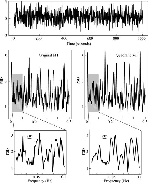
Spectrum estimation of pseudo-random number signal. The signal is a normally distributed random vector, with N= 1000 samples. The top panel shows the time-series random signal. The middle panels show the OMT (left-hand panel) and the QMT (right-hand panel) estimates of the spectrum. Bottom panels show a detailed view of the estimates between 0.01 and 0.1 Hz and the 2W bandwidth for reference. The QMT generates a smoother spectral estimate.

Open in new tabDownload slide

2

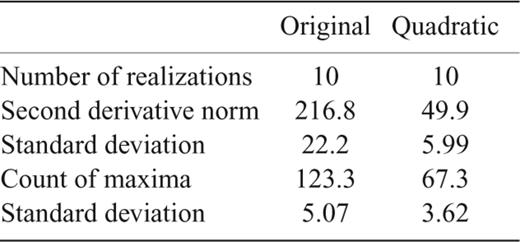
Comparison of smoothness for the multitaper methods.

Open in new tabDownload slide

Results of these measures of smoothness in Table 2 demonstrate that the QMT generates smoother estimates of the spectrum. In all 10 realizations, both measures of smoothness where lower when using the Quadratic method.

6.2 Periodic components

We test the effectiveness of the new method with two signals; we examine a random signal r(t) with σ= 1.0 and a pair of periodic components. The number of data points is reduced to N= 100 in order to have a comparison of spectral leakage around the linear components.

Our first test is to see whether this method represents the periodic components in the signal better, without introducing additional spectral leakage. For this, we take the signal:

35

where f₁= 0.05, f₂= 0.3 and the amplification factor A₀= 10⁵. Two questions arise here. How well can we describe the periodic components; effectively, line features in the spectrum, and is there any spectral leakage introduced due to the Quadratic multitaper method?Fig. 6 shows the results of spectral analysis from both OMT (grey) and QMT, on linear and log axes. The linear plot clearly shows the more accurate description of the periodic components provided by the QMT, the logarithmic plot shows that no additional spectral leakage is introduced. Note how both methods overlap at very low amplitudes. The signal has 8–10 orders of magnitude dynamic range and both methods behave similarly in terms of spectral leakage.

Figure 6

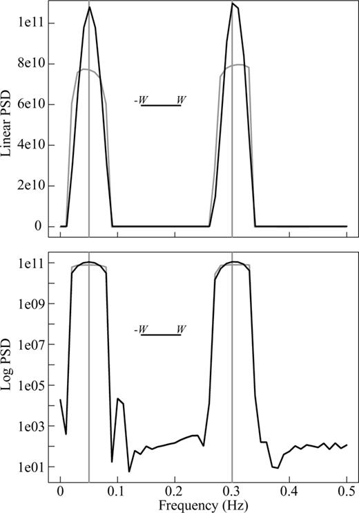
Spectrum estimation for a high dynamic range signal with two periodic components at 0.05 and 0.3 Hz. N= 100 points, time-bandwidth product NW= 3.5 and K= 6 . The linear scale spectrum (top panel) shows the improved performance of the QMT in describing the periodic components, while the logarithmic scale (lower panel) shows the similar spectral leakage properties of both methods.

Open in new tabDownload slide

The second test signal has a much smaller signal-to-noise ratio. In this case we let the amplification factor be A₀= 1.0 and the standard deviation σ of r(t) remains fixed. Fig. 7 shows the result of spectral analysis on this signal. We would like to stress two important features that can be seen from these results. First, the linear components are better described by the QMT. Second, the information outside the range of the periodic components is smoother, as shown in the random signal example (Table 2).

Figure 7

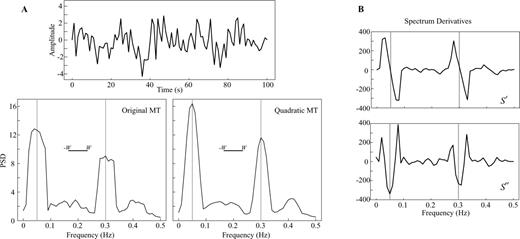
Spectrum estimation of a normally distributed random signal with two sinusoids at 0.05 and 0.3 Hz. Parameters as in Fig. 6. Plots below the time-series contain the estimates of the spectrum using the OMT (left-hand panel) and the QMT (right-hand panel). The figures in the bounded box (right-hand panel) show the first and second derivatives as estimated from the covariance matrix. Vertical grey lines represent the location of the line components. Note how the derivative estimates help in pinning where the line components are located.

Open in new tabDownload slide

Additionally, we have also obtained extra information about the spectrum. Fig. 7 shows the estimate of the first and second derivatives of the spectral contents of the signal. As expected, the first derivative should be very close to zero, when getting close to the periodic component. Similarly, the second derivative of the spectrum should have a large negative value, showing that the line represents a local maxima of the spectrum. These two features are clearly present in the estimates of the derivatives. Given the randomness of the signal and also uncertainties due to the non-uniqueness of the problem in our example, the second derivative around the 0.3 Hz components is not exactly the largest negative value, but is rather off by a frequency bin. This shows that still some uncertainties remain in all estimates, including the spectrum and its derivatives. Nevertheless, the extra information that is gained from the derivatives could certainly be relevant.

Note that the estimates of the derivatives are not computed by a numerical differentiation of the spectrum estimate , but rather by the steps described in the previous sections.

A method for the detection of periodic components using the multitaper method was developed by Thomson (1982), known as the F-test for spectral lines. For a complete description of the methodology the reader is referred to Thomson (1982) and Percival & Walden (1993). The method can be applied for reshaping the spectrum near spectral lines (e.g. Park 1987a; Thomson 1990; Denison 1999) or even for removal of these periodic signals embedded in a coloured spectrum (Percival & Walden 1993, Chap. 10; lees 1995). For high signal-to-noise ratios as in Fig. 6, F-test or other line detection methods are preferred for harmonic analysis.

The general idea of spectral reshaping is to subtract the effect of the statistically significant lines from the eigencomponents Y_k (see eq. 23). This subtraction is done before the adaptive weighting in eqs (25) and (26), meaning that it is possible to perform either OMT or the QMT estimates on the remaining stochastic part of the spectrum (without the deterministic periodic components, just removed), with similar improvements as presented in the examples above, if the Quadratic multitaper method is applied.

6.3 Resolution test and the choice of multitaper parameters

One important question that remains unanswered in spectral analysis using multitaper methods is, what is the optimal choice of the time-bandwidth product NW (the averaging bandwidth) and the number of tapers K (the more tapers, the smoother the estimate)? Or, having a chosen bandwidth W, what is the ideal number of tapers that should be used?Riedel & Sidorenko (1995) invented the sine multitaper method to get around this problem by choosing an optimal number of tapers iteratively at each frequency.

In the multitaper method literature, it has been proposed that K= 2NW− 1 as an appropriate choice, since the eigenvalues λ_k are all close to unity. This choice is essentially based on the leakage properties of the tapers, but does not take into account the particular shape of the spectrum of the signal under analysis. In this subsection, we present a comparison of the effect of the choices of NW and K on the resolution of the spectra around a periodic component. We show how the QMT is less dependent on these choices compared with OMT.

In Fig. 8 and Table 3, we compare the resolution of OMT and the Quadratic multitaper method. A useful criterion is that of the width of the half-power points, also known as the 3-dB bandwidth. This criterion reflects the fact that two equal-strength periodic components separated by less than the 3-dB bandwidth will show in the spectrum as a single peak instead of two (Harris 1978). We use the signal in the previous section (Fig. 6) and plot the spectrum centred on one of the periodic components on a dB scale defined as:

36

where f₀ is the frequency of the periodic component. We vary the time-bandwidth NW and the number of tapers K to investigate the effect of these choices. We also present in Table 3 the result of the 3- and 9-dB (th power) bandwidths for the different choices of NW and K by applying a linear interpolation.

Figure 8

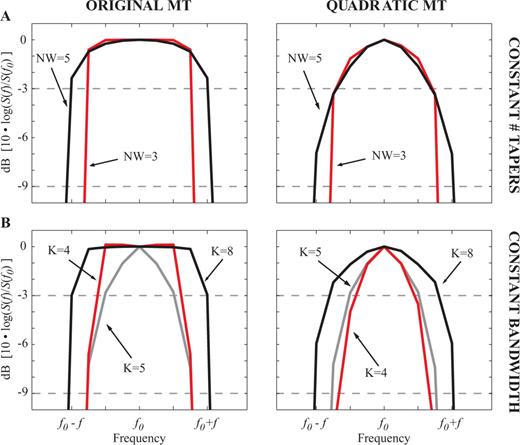
Resolution test comparison between OMT and the QMT with different choices of time-bandwidth product NW and number of tapers K for a periodic component in the spectrum in Fig. 6. In A we plot the spectral shape around a periodic component at frequency f₀ for two choices of time-bandwidth product NW with K= 7 tapers using the two methods. Two dashed lines represent the 3-dB (half-power) and 9-dB lines. The QMT has a 3-dB bandwidth that is narrower than the equivalent multitaper estimate and is relatively independent of the choice of NW. In B we fix the time-bandwidth product NW= 4.0 and vary the number of tapers. For the same choice of parameters the QMT outperforms the OMT with a narrower 3-dB bandwidth. We added the Quadratic estimate using NW= 4.0 and K= 5 on both plots for reference (grey line), resulting in a similar resolution to that of the K= 4 OMT (red line on left-hand plot) showing that the QMT can effectively provide smoother estimates (by using more tapers) without the loss of resolution.

Open in new tabDownload slide

3

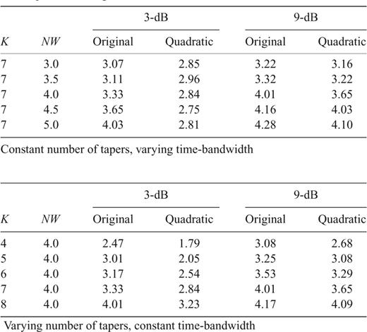
Comparison between multitaper methods by their 3- and 9-dB bandwidths in Rayleigh frequency f_R units with different choices of time-bandwidth product NW and number of tapers K for a periodic component in the spectrum in Fig. 6.

Open in new tabDownload slide

The QMT always outperforms the original method given the same parameters as shown in Table 3. Note that at the 9-dB line in Fig. 8 (see Table 3 as well) both methods provide similar results, with the method introduced here being slightly better.

An important result obtained by conducting this test is the fact that the 3-dB bandwidth is less sensitive to the choice of NW for the QMT (see Fig. 8a). Once we reach the 9-dB bandwidth, a larger value of NW decreases the resolving power. On the other hand the choice of K is directly proportional to the resolution bandwidth for both methods (this is also evident from Fig. 2), with the Quadratic method having narrower 3- and 9-dB bandwidths in all cases. A final observation from Table 3 indicates that a comparatively better resolution is achieved with the QMT even if one more taper K is used compared to OMT (compare also red and grey lines in Fig. 8b), leading to smoother estimates due to the increased degrees of freedom.

6.4 Synthetic earthquake signal

In geophysical applications many signals have a red spectrum with a large dynamic range but rarely with deterministic components (periodic signals). The spectra are continuous, for example the Earth's background seismic noise (Berger 2004), medium and small sized earthquake sources (e.g. Abercrombie 1995; Prieto 2004), the crustal magnetic field (Korte 2002), and many others.

Consider the spectrum of an earthquake, which follows the Brune (1970) model:

37

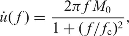
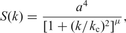
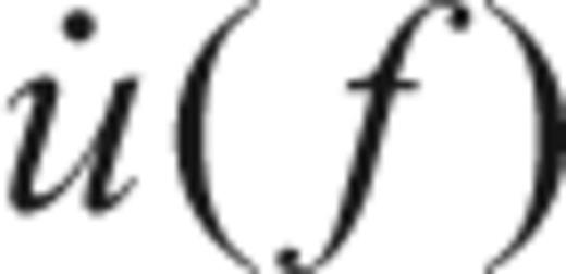where is the velocity amplitude source spectrum associated with the earthquake, M₀ is the seismic moment (related to the size of the earthquake) and f_c is the corner frequency. The corner frequency represents the predominant frequency content of the radiated seismic energy from the earthquake rupture. The spectrum from this model has a triangular shape if plotted in log–log axes with a slope of two in power.

In this synthetic example, we generate a pseudo-random time-series with 1000 samples whose spectra follow the source model in eq. (37). Even though OMT possesses good spectral leakage reduction, the spectrum may be biased due to the quadratic effects we discussed previously. This is especially true when the corner frequency gets extremely close to the sampling frequency, so that the curvature around f_c is described by a small number of spectral points.

Fig. 9 shows the spectral estimates from a realization of a synthetic source model with f_c= 0.005 Hz using OMT and the QMT. The triangular shape that is expected from source spectra is better constraint using the new method.

Figure 9

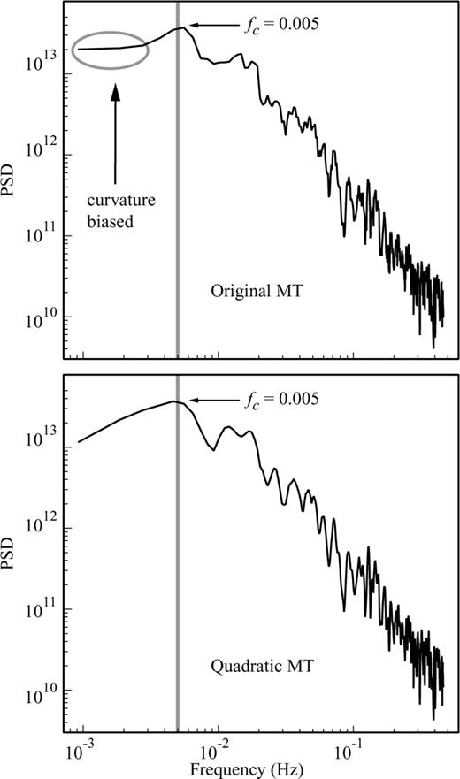
Spectrum analysis of synthetic earthquake model. The time-series (not shown) has 1000 samples (N= 1000) and we use time-bandwidth product of 3.5. The corner frequency f_c= 0.005 Hz (shown by an arrow) is to be estimated from the computed spectrum. Note how OMT biases the lower frequency part of the spectrum and does not resemble the triangular shape expected for these kind of signals. The QMT reduces the bias at lower frequencies considerably and is a better description of the shape of the spectrum around f_c.

Open in new tabDownload slide

In addition to the standard spectrum, it is also possible to obtain an estimate of the derivative of the spectrum. The derivative estimate of two different source models are shown in Fig. 10, taken from an average of 100 random realizations and corresponding standard errors. The two cases presented have corner frequencies close to the Rayleigh frequency f_R. Whenever the corner frequency is close to the sampling frequency, its curvature is represented by few spectrum bins.

Figure 10

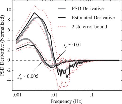
Mean derivative of the spectrum from 100 random realizations and two standard error bounds for two different earthquake models (see eq. 37), with corner frequencies f_c= 0.005 and 0.01 Hz. Time-series analysed is 1000 samples long. Note how the estimate closely resembles the model. In the case of the lower corner frequency, there is considerable bias at the lower frequency band.

Open in new tabDownload slide

The uncertainties of the derivative estimate are, similar to the uncertainties of the PSD, proportional to the amplitude of the spectrum. Using the derivative provides additional degrees of freedom for estimating parameters from the specrum.

6.5 Bathymetry profiles

A simple, isotropic, three-parameter model for the power spectrum of marine topography has been proposed of the form (Goff & Jordan 1988):

38

where a is the amplitude of the total root-mean-square roughness of the topography, k= |k| is the wavenumber, μ > 1 is the slope in the roll-off in the short wavelength part of the spectrum, and k_c is the corner wavenumber. We decided to use bathymetry data, given their more closely isotropic behaviour (stationarity in terms of time-series) and the availability of very high quality data sets.

We used bathymetry data obtained in the Central Pacific region (See Fig. 11), drawn from ship multibeam data (see also Marine Geoscience Data System, Macdonald 1992). From the available data we chose five profiles (east–west directions), four of them crossing the mid-ocean ridge, the other along the transform fault.

Figure 11

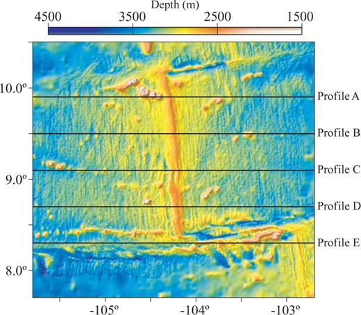
Location of the study area, where the profiles were taken from. Four of these profiles run across the mid-ocean ridge, and one is parallel to the transform fault. Location of the profiles is shown as thick black lines.

Open in new tabDownload slide

The idea of this example is to show what extra information can be extracted via the QMT. The bathymetry profiles have a sampling rate of 500 samples per deg and a total of 1251 samples per profile. The location of the profiles is shown in Fig. 11.

Fig. 12 shows the QMT analysis of the selected profiles. The spectrum is shown to have a large dynamic range (about seven orders of magnitude) over the entire frequency range. We focus our attention at the lower frequency range, where the corner wavenumber is expected from the model in eq. (38). The spectral shapes are very similar for all profiles and the different k₀ values are hardly distinguishable. An independent observation of the different behaviour between profiles can be drawn from the derivative estimates. See Fig. 12 and caption for discussion.

Figure 12

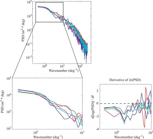
Spectral analysis of five selected profiles of bathymetric data in the Central Pacific Ocean around 9°N (see map in Fig. 11). QMT (left-hand plots) show very similar behaviour of the spectra. In addition to the standard spectra, the method provides an estimate of the derivative of the spectra (right-hand plot). We show the scaled derivative (approximately the derivative of ln (PSD). Note that the spectra can be grouped according to the derivatives, with one profile having a quite different behaviour (magenta line) showing a lower corner frequency. This derivative corresponds to profile E in Fig. 11, which samples the transform fault; while the rest of the profiles sample the mid-ocean ridge.

Open in new tabDownload slide

From the methods described above, we can obtain estimates of the derivative of the spectrum, and by normalizing by the spectrum,

39

we have an estimate of the derivative of the log spectrum (Thomson 1994). The derivatives also provide the means for comparing the different profiles, and clearly show the presence of two groups with particular spectral characteristics. This suggests that the profiles sampling the transform fault posses a lower corner frequency than the profiles sampling the mid-ocean ridge structure.

7 CONCLUSIONS

Multitaper spectral analysis is the method by which the data are multiplied by a set of orthogonal (in time and frequency) sequences, all having good spectral leakage properties. The sequences have the property of concentrating within a band 2W the frequency content of the spectral estimate. A simple average of the eigenspectra is not ideal, given the large dynamic ranges of some signals, and an adaptive weighting function is necessary, especially in regions where the spectrum has low amplitudes, and thus is prone to leakage from frequencies that have much larger amplitudes.

As noted by Riedel & Sidorenko (1995) and confirmed in this study, in regions where spectral leakage is not expected, corresponding to the regions of the spectrum with large amplitudes, the local or quadratic bias can have an important effect on the shape of the spectrum.

We introduce the Quadratic multitaper method, which estimates the derivatives of the spectrum, that is, the slope and curvature of the spectrum on the interval (−W, W) by solving a parameter estimation problem relating the derivatives of the spectrum and the K eigencomponents.

With the estimation of the second derivative (the curvature of the spectrum), we can apply a correction to the spectrum to obtain a new estimate that is unbiased to quadratic structure. This method reduces to the original Thomson (1982) multitaper estimate when the spectrum is locally flat in the interval (−W, W).

We present a variety of examples that indicate that the Quadratic multitaper method provides a smoother, less biased spectral estimate of the data as well as independent estimates of the derivatives of the spectrum. The information contained in the slope estimates can readily be applied in parameter estimation, or as an additional discriminant to compare two signals. No additional spectral leakage was introduced in the examples shown in this study.

We also discuss the effect of chosen multitaper parameters such as the time-bandwidth product and the number of tapers to compute. Even though it is still a user-defined set of parameters, we show that the Quadratic multitaper method leads to increased resolution compared to OMT and it is less dependent on the choice of the time-bandwidth in the inner interval. It allows the use of more tapers without the loss of resolution power compared to the original multitaper method.

Finally, model parameters can be found by analysing the goodness-of-fit between a Quadratic spectral estimate plus the slope of the spectrum of a data set with a theoretical model of the spectrum and its derivative. Another approach would be to generate from the theoretical model a covariance matrix C_jk (as in eq. 28) and find the model that best fits the data. In the later case, the information is not restricted to curvature; rather all information from the theoretical models is used.

ACKNOWLEDGMENTS

We thank David Sandwell and J. J. Becker for providing the bathymetry data used here. We would also like to thank one anonymous reviewer for constructive comments that helped improve the paper. Funding for this research was provided by NSF Grant number EAR0417983.

APPENDIX A: QUADRATIC MEAN-SQUARE ERROR

In eq. (33), a correction for the curvature or quadratic bias is applied to the multitaper estimate. In Section 5, we defined the expected value of the spectrum as an average over the inner interval (−W, W):

(A1)

and by applying the correction in 33, we have the expected value of the Quadratic multitaper estimate

(A2)

where we assume that .

The bias of the Quadratic multitaper is then

(A3)

and the variance, using the rules of propagation of errors (Taylor 1997) in eq. (33),

(A4)

and we can now define the mean square error (bias²+ variance):

(A5)

where the first term is the bias squared and the two on the right represent the variance. It is assumed that the covariance is insignificant. Taking the derivative with respect to μ and setting to zero

(A6)

and rearranging yields

(A7)

which is the solution shown in 34, using α₂ as estimates of S″.

To obtain the variance of the estimates and in the least squares problem (31), we compute the covariance matrix of the coefficients, following Lawson & Hanson (1974).

REFERENCES