


Abstract
The rifting history of the Atlantic continental margin of Newfoundland is very complex and so far has been investigated at the crustal scale primarily with the use of 2-D seismic surveys. While informative, the results generated from these surveys cannot easily be interpreted in a regional sense due to their sparse sampling of the margin. A 3-D gravity inversion of the free air data over the Newfoundland margin allows us to generate a 3-D density anomaly model that can be compared with the seismic results and used to gain insight into regions lacking seismic coverage. Results of the gravity inversion show good correspondence with Moho depths from seismic results. A shallowing of the Moho to 12 km depth is resolved on the shelf at the northern edge of the Grand Banks, in a region poorly sampled by other methods. Comparisons between sediment thickness and crustal thickness show deviations from local isostatic compensation in locations which correlate with faults and rifting trends. Such insights must act as constraints for future palaeoreconstructions of North Atlantic rifting.
1 Introduction
Offshore Newfoundland, eastern Canada, is an ideal research target for investigating the fundamental processes of continental extension, rifting, the opening of ocean basins and the related development of sedimentary basins. With oil and gas discoveries in the basins offshore Newfoundland, there exists an enhanced interest in developing a more complete geological understanding of the region. To that end, many geophysical surveys have been acquired by research institutions and by the exploration industry. Recently, the continental margin was drilled in the Ocean Drilling Project (ODP) to contribute complementary ground truth (Shipboard Scientific Party 2003). Nonetheless, many gaps in our knowledge remain about the structure of the Newfoundland margin, particularly at lithospheric scales. While several deep 2-D seismic reflection and refraction surveys have been acquired (Fig. 1A) (Keen et al. 1987a,b; Keen & de Voogd 1988; Todd et al. 1988; Reid & Keen 1990a,b; Reid 1993; Chian et al. 2001; Funck et al. 2003; Hopper et al. 2004; Lau et al. 2006a,b; Shillington et al. 2006; van Avendonk et al. 2006), which have demonstrated significant along-margin variability, few tie-lines exist to confidently track deep structures from profile to profile. Consequently, our 3-D view of the margin is incomplete.
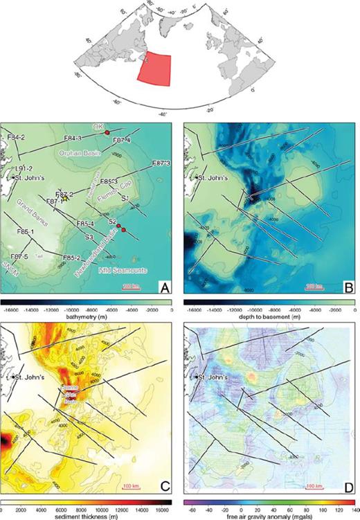
Maps of (A) bathymetry, (B) depth to basement, (C) sediment thickness and (D) free air gravity anomalies for the study region. A location map is plotted at the top of the figure with the study area shown as the red box. On all of the study area maps, the locations of deep seismic profiles acquired over the margin are indicated with black lines outlined in white. Seismic line labels in (A) are from the Frontier Geoscience Project (F), from the SCREECH experiment (S) and from Lithoprobe East (L). Key bathymetric structures of the margin are labelled in grey on plot (A) as are the location of the Hibernia oil field (yellow star) and the locations of ODP drilling sites (red circles). The location of the Jeanne d'Arc Basin is shown on plot (C). Abbreviations: SNTM, southern Newfoundland transform margin; OK, Orphan Knoll.
Potential field methods provide a tool for bridging gaps in seismic coverage and tracking deep structures regionally. With the development of algorithms for 3-D inversion of gravity data which can incorporate geological and geophysical constraints (e.g. Li & Oldenburg 1998), a regional density anomaly model of the margin can be constructed which satisfies geometrical constraints from existing seismic profiles and which provides information about unsampled regions. In this study, we undertake constrained 3-D gravity inversion of the free air data collected over the Newfoundland margin to generate a 3-D density anomaly model of the region. This density anomaly model serves to extend our knowledge about Moho topography and crustal density structure across the margin and to provide a better framework for understanding the geodynamics of rifting.
2 Tectonic Setting
Stabilized at the end of the Appalachian Orogen, the basement rocks of the Newfoundland margin consist of Precambrian and Palaeozoic rocks of the Avalon terrane (Enachescu 1987). During the Late Triassic, extensional forces thinned these basement rocks along major listric faults, producing the many half-graben basins of the Grand Banks, and isolating the Flemish Cap, a block of 30-km-thick continental crust located northeast of the Grand Banks and interpreted as an extension of the Avalon terrane (Enachescu 1992). From Late Jurassic to Early Cretaceous, extension spread outboard of the Grand Banks and Flemish Cap, evolving into the rifting that separated Newfoundland from Iberia and creating the modern North Atlantic Ocean. The transform fault marking the southern boundary of the Grand Banks resulted from a slightly earlier rifting event at 175 Ma as Nova Scotia/North America separated from Morocco/Africa (Haworth & Keen 1979; Klitgord & Schouten 1986). During this rifting, part of the African Meguma terrane was left behind in North America, making up the southern extent or tail of the Grand Banks (Haworth et al. 1994). Rifting north of the transform progressed from south to north with the first oceanic crust in the study region being generated to the southeast of the Grand Banks at 122 Ma, to the northeast of Flemish Cap by 109 Ma and finally to the NNW of the Orphan Basin by 84 Ma (Ziegler 1989). As rifting propagated northward, its strike changed from N—S to ENE—WSW immediately to the south of Flemish Cap (Haworth & Keen 1979) and then to WNW—ESE north of Flemish Cap. Eventually, during the Late Cretaceous to the Tertiary, post-rift subsidence became the dominant tectonic activity.
Despite evidence of limited localized volcanism, the Newfoundland-Iberia conjugate margin is classified as non-volcanic and the rift is thought to have been slow-spreading with faulting of the cool thinned brittle crust contributing to the serpentinization of the underlying mantle (Pérez-Gussinyé 2001). In cross-section, the rifted margin consists of extended continental crust making up the continental shelf, the continental slope, transitional crust and finally, oceanic crust in the deep water environment. The width of this zone of transitional crust varies along the margin, at its widest to the east of the central Grand Banks (80 km according to Lau et al. 2006a) and narrowing to the south on the tail of the Grand Banks (absent according to Keen & de Voogd 1988) and to the north towards Flemish Cap (60 km immediately south of Flemish Cap according to Shillington et al. 2006, and absent off Flemish Cap according to Funck et al. 2003).
3 Gravity Data
Free air gravity data over the Newfoundland margin are readily available from both land-based and shipboard gravity soundings as well as from closely spaced satellite altimeter surveys. The full coverage used for this study is shown in Fig. 1(D) and consists of 193 532 data points. The satellite gravity data are evenly distributed throughout the study area whereas the ship track data stand out in Fig. 1(D) as denser lines with the densest concentration of ship track data located over the northeast portion of the Grand Banks, a region of major hydrocarbon discoveries such as the Hibernia field (yellow star in Fig. 1A) within the Jeanne d'Arc Basin.
Onshore and offshore gravity mapping has been undertaken by the federal government of Canada since 1944 with the majority of data coming from dynamic gravimeters aboard moving ships. These soundings are adjusted in a least-squares sense to the control stations of the International Gravity Standardization Network 1971 (Morelli et al. 1974). The Canadian Geodetic Information System of the Gravity and Geodetic Networks Section of Geomatics Canada freely provides digital point data of these measurements on the internet (http://gdr.nrcan.gc.ca/gravity). Gravity anomalies from satellite altimetry data are available from a compilation of the results from the Geosat Geodetic Mission and the ERS 1 Geodetic Phase mission (Sandwell & Smith 1997). These data can be downloaded from Scripps Institution of Oceanography (http://topex.ucsd.edu/).
In general, the free air gravity anomalies over the Newfoundland margin are positive with negative anomalies constrained to the Orphan Basin, Flemish Pass, the Jeanne d'Arc Basin and portions of the Grand Banks closest to the mainland. Curiously, the strongest positive free air gravity anomaly on the margin, located 200 km east of St. John's, overlies a very deep sedimentary basin containing over 10 km of low density sediments. Grant (1987) has interpreted this gravity high as resulting from a dense body of unknown origin beneath the sedimentary basin.
The free air gravity data over the Newfoundland margin have not been extensively studied. Apart from qualitative observations in regional studies (e.g. Haworth et al. 1994), quantitative studies have been limited to areal filtering to detect trends (Miller & Singh 1995) and forward modelling and inversion of the gravity data along colocated 2-D seismic profiles (e.g. Keen & Dehler 1997; Funck et al. 2003). A previous study involving 3-D gravity inversion over the Grand Banks (Morrissey 2001) was unable to take advantage of additional recent seismic data. Otherwise, the regional distribution of gravity anomalies and their corresponding 3-D density anomalies along this margin have not been modelled. In this manuscript, we develop such a model from the free air gravity data point measurements (Fig. 1D) using a 3-D gravity inversion algorithm and both bathymetric and sediment thickness constraints (Figs 1A and C). Geometrical constraints from multiple 2-D seismic profiles are used to gauge the quality of the inversion results.
4 3-D Gravity Inversion
Gravity forward modelling involves computing the gravitational response from a prescribed density anomaly model. Conversely, gravity inversion involves generating a density anomaly model directly from an observed gravitational response. While the resulting model is non-unique and simply represents one of many models that can satisfy the observations, the inversion can be constructed so as to generate a specific type of model that conforms to the expected layout of the subsurface. The incorporation of model constraints from other complementary techniques can further hone the inversion process and generate more realistic density anomaly models.
The GRAV3D modelling algorithm, developed by Li & Oldenburg (1996, 1998), is a robust 3-D gravity inversion code which easily allows the incorporation of a priori model information from other techniques. The algorithm inverts gravity observations at the Earth's surface to obtain a subsurface 3-D density anomaly distribution (relative to a background density of 2670 kg m−3) below the observation locations. Since gravity data inherently do not contain depth information, the algorithm applies a depth weighting function to the resulting density anomaly distribution to account for the natural decay of the resolution kernels with depth and to prevent the inversion from concentrating the density anomalies at the surface of the model.
The GRAV3D mesh onto which the 3-D density anomaly distribution is modelled consists of rectangular prisms of arbitrary size with a constant density anomaly assigned to each prism. For this study, the mesh was constructed from flattened cubes with lateral dimensions of 15 km × 15 km and 500 m deep. The horizontal extent of the mesh corresponded to the study area shown in Fig. 1 and contained 65 cells in both the easting and northing directions. The vertical extent of the mesh, however, required more careful consideration and will be discussed later in the inversion section.
The GRAV3D inversion is formulated as an optimization problem which balances the degree to which the desired type of model can be generated (model norm) and the degree to which the inverted model can reproduce the observed data within their error bounds (misfit). The model norm is described in terms of directionally dependent smoothing length scales which can generate any range of model types (e.g. small, flat, blocky). The model norm can be further adapted to minimize the difference between the inverted density model and some reference density model. Meanwhile, the misfit is a least-squares measure of the difference between the observed gravity values and those predicted from the inverted density anomaly model. The difference is further weighted by the reciprocal of the observed data errors such that the target misfit for the inversion is unitless and should be equal to the number of data points provided that the data errors are independent and Gaussian with zero mean (Li & Oldenburg 1998).
The gravity data used in the inversion are the free air gravity point measurements shown in Fig. 1(D). The lack of data around the edge of the study area corresponds to the location of the padding cells in the mesh. For the land-based and shipborne data, all data corrections were performed by Natural Resources Canada and the error estimates for these corrections were provided with the data. These estimates, which ranged from 0.1 to 5.1 MGal, reflect the accuracy of the free air anomaly computation rather than uncertainties in the data measurements themselves. For the satellite altimeter data, the accuracy of the gravity anomalies ranges from 4 to 7 MGal based on comparisons with ship track data (Sandwell & Smith 1997). Since the downloaded satellite gravity anomalies were not assigned specific errors for each data point, we have arbitrarily assigned an error of 5 MGal to each of the measurements.
For our inversion, we opted for GRAV3D to generate a 3-D density anomaly model that was smooth over length scales of 150 km in the easting and northing directions and smooth over a length scale of 6 km in depth. In terms of fitting the data, given the coarseness of the mesh and the dense data coverage, we opted to relax the acceptable misfit value to 10 times the number of data points. Multiple test inversions using lower misfits resulted in overly structured density anomaly models that bore less resemblance to models from complementary geophysical methods.
4.1 Constraints
The GRAV3D algorithm is very flexible when incorporating a priori model information. Using a reference density anomaly model, the inversion algorithm can be customized such that the density anomaly within a given prism can be restricted to only vary within a set range of values and the degree of variability can differ for each prism independently. In this way, features of known density such as ocean water can be incorporated directly into the reference density anomaly model and remain unaffected during the inversion. In other words, regions of the model which are well defined and whose densities are known from other techniques can be ‘hard-wired’ into the model.
Bathymetric data for the Newfoundland margin, gridded at 500 m, were obtained from the Geological Survey of Canada. These data were incorporated into the reference density anomaly model by forcing all model prisms above the bathymetric depths to contain density anomalies corresponding to ocean water (−1640 kg m−3 relative to a background density of 2670 kg m−3). During the inversion, the density anomaly in these prisms was only allowed to vary between −1600 and −1680 kg m−3, essentially keeping them fixed. This approach of incorporating ocean water directly into the reference density anomaly model differs from earlier 3-D gravity inversion studies over water where the influence of the ocean water is estimated and subtracted from the observed free air gravity data prior to the inversion (Flores-Marquez et al. 2003). We feel that the direct incorporation of ocean water into the density anomaly model is advantageous in that there are no water correction errors incorporated into the inversion.
Using seismic imaging results from intensive exploration of the Newfoundland margin's sedimentary basins by the oil and gas industry and by academia, Grant (1988) compiled a depth to crystalline basement map for offshore eastern Canada. The digitized depth to basement values from this map were provided by the Geological Survey of Canada and used to generate the map in Fig. 1(B). Combining the depth to basement with the bathymetric information, a map of sediment thicknesses was constructed across the margin (Fig. 1C). This information was then incorporated into the reference density anomaly model by assigning a density anomaly of −400 kg m−3 (relative to a background density of 2670 kg m−3) to the prisms lying between the seabed and the basement. For the inversion results presented in this manuscript, the density anomaly in each of these prisms was allowed to range between −600 and −200 kg m−3, corresponding to a range in densities of 2070–2470 kg m−3. This range of density anomaly values was chosen to force the prisms to contain reasonable densities for sedimentary rocks while allowing the inversion to stratify (as needed) the densities within the sedimentary column and within individual basins. In order to test the sensitivity of the inversion to our choice of density range for the sedimentary rocks, we ran two test inversions, one where the density anomalies were allowed to range between −600 and 0 kg m−3 (corresponding to a range in densities of 2070–2670 kg m−3) and another more extreme example where the density anomalies were allowed to range between −600 and 200 kg m−3 (corresponding to a range in densities of 2070–2870 kg m−3). By allowing for higher density anomalies within the sedimentary basins, the resulting density anomaly models required less mass below the basins to reproduce the gravitational signal and so resulted in the deepening of the Moho beneath deeper sedimentary basins by 2–3 km. These tests must be kept in mind when considering the inversion results above deep sedimentary basins (where higher density anomalies are appropriate) presented in this manuscript. While it would have been preferable to assign sedimentary densities into the model using geophysical density well logs, only a small number of wells drilled along the margin extend to basement and none of these have corresponding density logs available to us. Consequently, we feel that our approach of constraining the density anomaly values within sedimentary mesh prisms is the most appropriate and flexible given the lack of other constraints.
Once the ocean water and sedimentary portions of the reference density anomaly model were assigned, all remaining mesh prisms were assigned a density anomaly of 0 kg m−3 (corresponding to the background density). During the inversion, the density anomaly in each of these prisms was allowed to vary between –400 and 800 kg m−3 (corresponding to a range in densities of 2270–3470 kg m−3). Thus, below the base of sediments, the inversion was given great flexibility in assigning density anomalies to reproduce the observed gravity response and no constraints were placed on which prisms should correspond to crustal rocks (with density anomalies of approximately less than 350 kg m−3) and which prisms should correspond to upper-mantle rocks (with density anomalies of approximately greater than 350 kg m−3).
4.2 Seismic corroboration
The 2-D crustal-scale seismic reflection and seismic refraction/wide-angle reflection profiles acquired over the Newfoundland margin cannot easily be incorporated as constraints into the reference density anomaly model due to their sparse sampling of the margin (Fig. 1A). However, they can contribute to appraising the inverted results, particularly along profiles for which depth constraints exist (e.g. from seismic refraction modelling, from 2-D gravity modelling or from depth conversion of seismic reflection sections). These seismic profiles can also provide valuable corroborating evidence where they intersect anomalous features resolved from the gravity inversion and can supplement information at depths below the inverted density anomaly model. The seismic profiles most relevant to the discussion in this manuscript were acquired as part of the Frontier Geoscience Project (FGP), the Study of Continental Rifting and Extension on the Eastern Canadian SHelf (SCREECH) project and from various seismic refraction/wide-angle reflection surveys conducted by the Geological Survey of Canada (GSC) prior to and as part of the Lithoprobe project.
The Geological Survey of Canada's Frontier Geoscience Project, which operated from 1984 to 1990, undertook the acquisition of almost 7000 km of 2-D crustal-scale multichannel marine seismic reflection data over the margin of eastern Canada. The FGP profiles relevant to the Newfoundland margin are plotted on Fig. 1(A). While many of these profiles are only available as time sections [F84-2 (Keen et al. 1986), F85-1 (Keen et al. 1987a), F87-1 (de Voogd et al. 1990), F87-2 (de Voogd et al. 1990)], other profiles were also the site of seismic refraction profiling and/or 2-D gravity modelling and consequently provide depth constraints [F84-3 (Chian et al. 2001), F85-2 (Reid 1994), F85-3 (Reid & Keen 1990a), F85-4 (Reid & Keen 1990b), F87-5 (Todd et al. 1988)]. Prior to the FGP project, the Geological Survey of Canada had conducted two seismic refraction experiments in the Orphan Basin and Flemish Pass providing a few sparse constraints on Moho depth and crustal velocity (Keen & Barrett 1981). Following from the FGP project, Lithoprobe acquired the L91-2 seismic refraction profile as part of the Lithoprobe-East transect, supplementing the FGP results (Marillier et al. 1994).
The most recent SCREECH project undertaken in 2000, was a joint US-Canadian-Danish collaborative project between Woods Hole Oceanographic Institution, the University of Wyoming, the Danish Lithosphere Centre, Dalhousie University and Memorial University of Newfoundland. The project involved the acquisition of multichannel seismic reflection and seismic refraction/wide-angle reflection data along three main profiles (labelled S1, S2 and S3 in Fig. 1A). The velocity structural models developed from the seismic refraction data provide further depth constraints for the margin (Funck et al. 2003; Lau et al. 2006a; van Avendonk et al. 2006).
4.3 Vertical extent of the mesh
For typical gravity inversions used in mineral exploration, the goal of the inversion is to produce density models that help delineate mineralized bodies of anomalous density within host rocks whose densities are close to the background density (2670 kg m−3). For these inversions, only the cells corresponding to the mineralized bodies will have density anomalies other than 0 kg m−3 and the addition of any extra cells with the background density will not influence the gravitational response. Consequently, the meshes can be made as large as is computationally reasonable without affecting the inverted results. Gravity inversions for crustal studies behave very differently. This is because densities within the Earth increase with depth such that the background density of 2670 kg m−3 only applies within the upper crust and the density anomalies below that become increasingly larger. As such, the choice of the maximum vertical extent of the inversion mesh becomes very important.
For any given gravity measurement on the surface of the Earth, there exists a specific mass excess or deficiency broadly distributed below the observation location which gives rise to that measurement. In the absence of any constraints, this mass excess or deficiency will be distributed vertically throughout the cells of the mesh below the observation. Thus, if the mesh is very short in height, the mass excess or deficiency will be spread over a smaller vertical depth extent such that each cell will have an artificially high density anomaly. Meanwhile, very tall meshes will contain artificially low density anomalies since these are spread over too large a vertical extent. Consequently, the total height of the mesh much be chosen carefully if the density anomalies are to be properly distributed and geologically reasonable.
In order to gauge the best maximum vertical extent for the mesh used in this manuscript, several test inversions were run with different maximum mesh depths (20, 25, 30, 35 and 40 km). Slices through the inverted density anomaly models corresponding to profile S3 are compared in Fig. 2. For all of these inversions, individual mesh cells were 500 m deep and the deeper meshes were constructed by adding more cells to the base of the mesh. For all slices, the seabed and the depth to the base of sediments were kept fixed and all other inversion parameters such as misfit and both horizontal and vertical smoothing were kept the same. The predicted gravitational signals from each of these models fit the observed gravitational signal equally well.
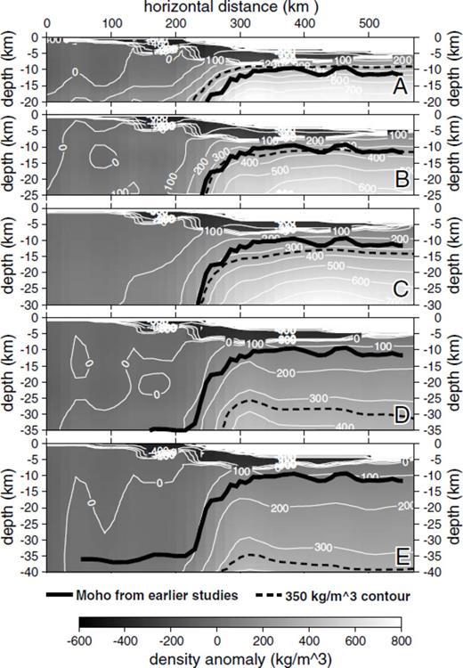
Influence of maximum depth extent of mesh on 3-D gravity inversion results compared along profile S3 from the SCREECH experiment for meshes extending to (A) 20 km, (B) 25 km, (C) 30 km, (D) 35 km and (E) 40 km depth. For all panels, the mesh cells were 500 m deep with the deeper meshes containing an increasing number of cells. The density anomaly values are relative to 2670 kg m−3. The bathymetry and the base of sediments are used to constrain the model and are kept fixed during the inversions. Overlain on the profiles are the Moho constrained from a seismic refraction/wide-angle reflection survey (Lau et al. 2006a) (solid black line) and the 350 kg m−3 contour used as a proxy for the transition from crustal to mantle densities (dashed black line).
The results presented in Fig. 2 clearly demonstrate that the choice of maximum mesh depth has a strong influence on the subsurface distribution of density anomalies. With a very short mesh, the inverted density anomalies are higher (Fig. 2A). As the vertical extent of the mesh is increased (Figs 2B—E), the anomalies within each individual cell are reduced while the greater number of cells still satisfies the required mass excess. From this point, picking the appropriate maximum vertical extent for the mesh depends highly on having other geophysical constraints.
Assuming that a density anomaly of 350 kg m−3 (absolute density of 3000 kg m−3) is appropriate for differentiating between crust and mantle densities, the 350 kg m−3 contour is highlighted with a dashed black line on the plots in Fig. 2. For comparison, the Moho constrained by seismic refraction/wide-angle reflection profiling along S3 (Lau et al. 2006a) is plotted as the solid black line. These two lines show the best match for the mesh that is 25 km deep. For deeper meshes, a similar match can only be achieved if we assume that a lower density anomaly (absolute density less than 3000 kg m−3) corresponds to the transition from crust to mantle.
It is important to note that increasing the mesh depth to 40 km and beyond does not reveal any density anomalies that can be interpreted as Moho beneath the thicker crust (Fig. 2E). This is because there is a maximum compensation depth below which the free air gravity at the surface is no longer sensitive to underlying density anomalies. While isostatic depth of compensation normally corresponds to, or is near, the base of the crust, Simpson et al. (1986) argued for a shallower depth of compensation for crust overlain by sea water, with density anomalies below that depth not contributing to the gravitational signal. Using the Airy-Heiskanen isostatic model to perform isostatic residual gravity calculations, they obtained a 30 km isostatic depth of compensation for the continental United States and showed that the isostatic depth of compensation would shallow offshore. Given the results shown in Fig. 2, we would argue for an isostatic depth of compensation of 25 km offshore Newfoundland and have limited the inversion meshes used in the remainder of this manuscript to that maximum depth. Moho topography at shallow levels (less than 25 km depth) is easily resolved while deeper Moho structure cannot be resolved using gravity inversion. By limiting the maximum depth of our mesh to 25 km and with each of our mesh cells having dimensions of 15 km × 15 km by 500 m deep, the resulting mesh was 50 cells deep.
4.4 Inversion results
By inverting for the free air gravity point measurements using our reference density anomaly model and the parameters outlined above, we generate a 3-D density anomaly model that is able to successfully reproduce the gravity observations along the Newfoundland margin (Fig. 3A). All of the main observed gravity features are reproduced and the magnitudes of the gravity field values match well. As with the observed data (Fig. 1D), the predicted anomalies are generally positive with negative anomalies constrained to the Orphan Basin, Flemish Pass, the Jeanne d'Arc Basin and portions of the Grand Banks closest to the mainland.
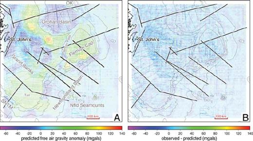
Predicted free air gravity anomaly map from the inverted density anomaly model (A) and the difference between these predicted data and the observed data shown in Fig. 1(D) (B). On both maps, the locations of deep seismic profiles acquired over the margin are indicated with black lines outlined in white. Key bathymetric structures of the margin are labelled in grey on plot (A). Abbreviations: SNTM, southern Newfoundland transform margin; OK, Orphan Knoll.
The overall fit between the observed and predicted gravity anomalies can be assessed by examining their difference plot (Fig. 3B). This plot shows that the differences are generally less than 20 MGal throughout the study region and that there are no regional trends. As such, the inversion managed to successfully reproduce all of the long-wavelength data trends. The shorter wavelength jitter in the difference plot are a direct consequence of our blocky mesh parametrization and of imposing the strict bounds on the ocean water and to a lesser extent on the sedimentary portions of the reference density model. Without the incorporation of those strict constraints, the resulting gravity anomaly predictions are much smoother while the resolved density anomaly model bears less resemblance to the subsurface as constrained from other methods. However, since we require a density anomaly model that stays true to our a priori information, the jitter remains an unavoidable artefact. Nonetheless, since the features of interest in this manuscript are much broader in scale than the jitter, these high frequency artefacts do not detract from our overall ability to interpret the inverted results.
4.4.1 Moho variations
The Moho depths resolved from the various 2-D seismic refraction and gravity modelling profiles from FGP, SCREECH, Lithoprobe East and other GSC projects were used to generate an interpolated Moho depth map for the Newfoundland margin (Fig. 4A). The interpolation was performed using the Generic Mapping Tools software (Wessel & Smith 1991) and involved the use of a continuous minimum curvature surface gridding algorithm. Despite the limited Moho depth constraints (white circles in Fig. 4A), the resultant map does show the deeper Moho and thicker crust of the Grand Banks and Flemish Cap but the variable seismic coverage leaves Moho depths in many regions suspect and biased by the interpolation routine.
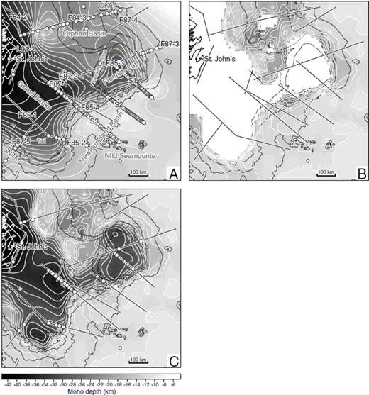
Maps of Moho depths, (A) interpolated from digitized Moho picks along seismic profiles and earlier 2D gravity models, (B) from the 350 kg m−3 anomaly isosurface of the inverted density anomaly model (regions without Moho constraints have been masked in white), and (C) from the combination of the isosurface in (B) with seismic constraints below 25 km depth in (A). On plots (A) and (C), the seismically constrained Moho pick locations used in the interpolation are shown as white circles. On all maps, the locations of deep seismic profiles acquired over the margin are indicated with black lines outlined in white. Seismic line labels as per Fig. 1. Key bathymetric structures of the margin are labelled in grey on plot (A). Abbreviations: SNTM, southern Newfoundland transform margin; OK, Orphan Knoll.
If we select a density contrast of 350 kg m−3 as a proxy for the Moho in our inverted density model and generate the corresponding isosurface, we obtain an inverted-gravity-constrained Moho model for the Newfoundland margin (Fig. 4B). Given that our inverted model does not extend below 25 km depth, the resulting Moho model is also restricted to 25 km depth. However, if we supplement the inverted Moho with the available seismic constraints below 25 km depth and interpolate in between, we obtain the hybrid Moho model illustrated in Fig. 4(C). In this map, the same continuous minimum curvature surface gridding algorithm that was used in Fig. 4(A) is used for the Moho regions below 25 km depth and the interpolation algorithm is constrained by the Moho depth constraints shown by the white circles.
The 3-D density anomaly model derived from the gravity inversion shows excellent agreement with the available seismic constraints. Fig. 5 shows slices through the density anomaly model along seismic profiles for which depth constraints are available. The corresponding plots comparing the observed and predicted gravity anomalies along these slices are presented in Fig. 6. On all these slices through the density anomaly model, the seismically constrained Moho is overlain as a thick black line. In general terms, the seismically constrained Moho on most of the profiles tracks the 350 kg m−3 contour of the inverted density anomaly model. The projections of the hybrid Moho model on the density anomaly model slices are shown as the dashed lines in Fig. 5.
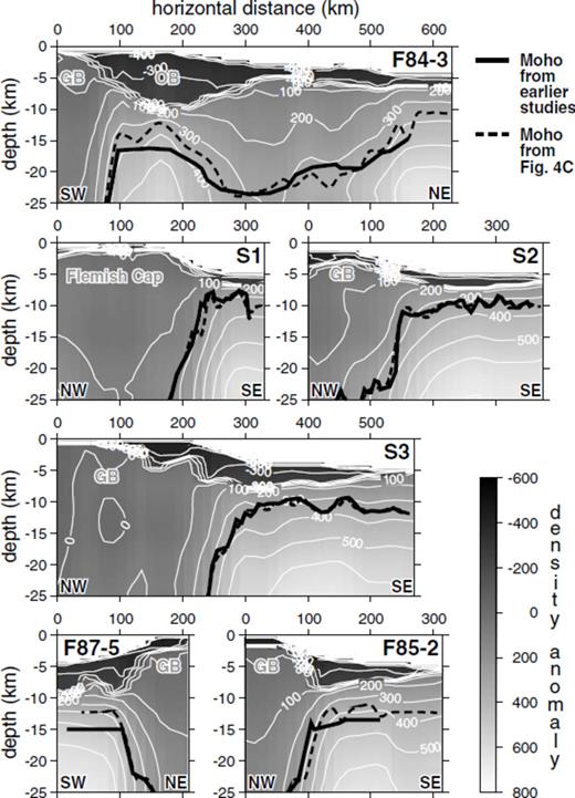
Slices through the inverted density anomaly model along seismic lines for which wide-angle seismic reflection/refraction and/or profile density modelling Moho constraints are available. The overlain thick dashed black lines correspond to the Moho depths obtained from Fig. 4(C) and the thick solid black lines correspond to the interpreted Moho depths published from other earlier studies. Line labels correspond to those plotted in Fig. 1(A). Key bathymetric structures of the margin are labelled in grey. Abbreviations: GB, Grand Banks; OB, Orphan Basin.
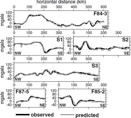
Comparison between the observed free air gravity anomalies (black lines) and the anomalies predicted for the inverted density anomaly model (grey lines) for the slices in Fig. 5.
The six profiles for which seismic constraints are available (Fig. 5) all show good correspondence between the seismically derived Moho and the hybrid Moho. The best fits are obtained along the three SCREECH profiles (S1, S2 and S3). For these profiles, the seismically constrained Mohos for S1 and S3 were obtained using PmP reflections (Funck et al. 2003; Lau et al. 2006a) while for S2, van Avendonk et al. (2006) defined the Moho as corresponding to the depth at which seismic velocities exceeded 8.0 km s−1. Further south along profile F85-2, the match between the hybrid Moho and the seismically constrained Moho is not quite as good with the hybrid Moho showing a greater amount of relief. This discrepancy may however just be due to the coarseness of the velocity model from which the seismically constrained Moho was obtained. Along profile F84-3 which extends NE from the Grand Banks across the Orphan Basin, the hybrid Moho generally matches very well with the Moho obtained using PmP reflections and profile gravity modelling (Chian et al. 2001) although there is a discrepancy beneath the thickest part of the Orphan Basin. This discrepancy of 2–3 km may simply be reflecting that our choice of maximum allowable density anomaly (−200 kg m−3) for the deepest sediments was slightly too low and should have been closer to the background density anomaly (0 kg m−3). Along the southwestern transform margin of the Grand Banks (F87-5), a similar discrepancy is observed between the hybrid Moho and the seismically constrained Moho although it does not mimic the variations in the overlying sediment thickness and thus may be implying that material in the seismically defined lower crust is of much higher density than expected.
Eight slices through the inverted density anomaly model along which no depth-converted seismic constraints are available are plotted in Fig. 7 with their corresponding plots of observed versus predicted gravity anomalies presented in Fig. 8. Since five of these profiles (L91-2, F84-2, F87-1, F87-2 and F85-1) extend across crust that is more than 25 km thick, no Moho comparisons can be made for these profiles. Meanwhile, the hybrid Moho (Fig. 4C) projections on the other three slices are plotted as dashed lines. For comparison, the projections of the interpolated seismically constrained Moho map (Fig. 4A) are plotted with the black dots outlined in white. The best correspondence between these two Mohos occurs along profile F85-4 which extends subparallel to profile S3 and cuts the margin at a slight angle. On the northeastern edge of the Orphan Basin, the slice through profile F87-4 shows a poor match at the SW end of the profile but the match improves to the NE. We believe that the hybrid Moho is more reliable in this region due to the small number of nearby seismic constraints. Lastly, profile F85-3 which crosses the Jeanne d'Arc Basin and the Flemish Cap generally shows a good correspondence at the NE end of the profile. The shallowing of the Moho beneath the Jeanne d'Arc Basin to approximately 16 km depth is not directly predicted by the seismically constrained Moho although some shallowing is observed immediately to the northeast. The only seismic constraint for this shallowing comes from the one Moho depth estimate to the north of the line in Flemish Pass (Keen & Barrett 1981).
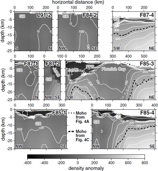
Slices through the inverted density anomaly model along seismic lines for which depth-converted Moho constraints are not available. The overlain thick dashed black lines on plots F87-4, F85-3 and F85-4 correspond to the Moho depths obtained from Fig. 4(C) while the black dots outlined in white are extracted from the seismically constrained interpolated Moho depth map in Fig. 4(A). Line labels correspond to those plotted in Fig. 1(A). Key bathymetric structures of the margin are labelled in grey. Abbreviations: GB, Grand Banks; OB, Orphan Basin; JdAB, Jeanne d'Arc Basin; FPB, Flemish Pass Basin.
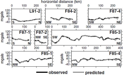
Comparison between the observed free air gravity anomalies (black lines) and the anomalies predicted for the inverted density anomaly model (grey lines) for the slices in Fig. 7.
As observed in the hybrid Moho map (Fig. 4C) and hinted at in the slice through profile F85-3, one of the most striking features to result from the 3-D gravity inversion is the extreme shallowing of the Moho to 12 km depth to the west of Flemish Cap and immediately to the north of the Jeanne d'Arc Basin. This shallowing which has not been previously recognized and is not currently constrained by any seismic results, is required by the inversion to reproduce the strong positive gravity anomaly observed 200 km to the east of St. John's (Fig. 1D). With the significant thickness of low density sediments at this location, higher density mantle material must be brought closer to the surface to compensate for the overlying sediments and reproduce the positive gravity high. While our choice of density anomaly limits for the sediments in the inversion directly impacted the depth of the resolved Moho, even with a higher density anomaly limit for the sediments, the Moho would still shallow to 15 km in this region. Thus, the dense body of unknown origin postulated by Grant (1987) to explain this gravity high appears to correspond to mantle material.
Profile F85-3 lies south of the extremely shallow Moho derived from the gravity inversion and crosses over its shallowing flank. Unfortunately, depth constraints from seismic refraction profiling along this line are confined to its eastern portion (Reid & Keen 1990a) and the seismic reflection results were never depth-converted (Keen et al. 1987a). One Moho depth estimate of 20–22 km is available just off the line in Flemish Pass (Keen & Barrett 1981), but otherwise, Moho depth constraints near the shallowing Moho are not available. A line drawing of the time section for profile F85-3 is shown in Fig. 9(A) and the Moho interpreted by Keen et al. (1987a) is overlain in blue on the identical time section in Fig. 9(B). Keen et al. (1987a) arrived at this interpreted Moho by extrapolating the clearly defined Moho beneath Flemish Cap westward through two widely spaced discrete pockets of reflectivity on the seismic section. If we coarsely interpret horizons for bathymetry and base of sediments (red and green lines, respectively, in Fig. 9B) and convert the horizons to depth using velocities of 1500, 4000 and 6500 m s−1 for water, sediments and crust, respectively, we obtain the depth horizons plotted in Fig. 9(D). While the bathymetry and base of sediment horizons show good correspondence with the density anomaly model, the interpreted Moho from Keen et al. (1987a) poorly fits the Moho obtained from the gravity inversion with the discrepancy between the two Mohos at its greatest where the seismic constraints are most poor. Bearing the inversion results in mind and qualitatively reinterpreting the seismic section along F85-3, we would argue that the seismic reflection results along profile F85-3 support a shallowing of the Moho beneath the Jeanne d'Arc Basin. If we allow the Moho to follow the arched trend of reflectivity at 7–10 s, we generate a Moho time horizon (purple line in Fig. 9B) that, when converted to depth, matches the hybrid Moho quite well (purple line in Fig. 9D). Without this upwelling of higher density mantle material, it would be impossible to reproduce the corresponding gravity high above the northern limit of the Jeanne d'Arc Basin (Fig. 9C).
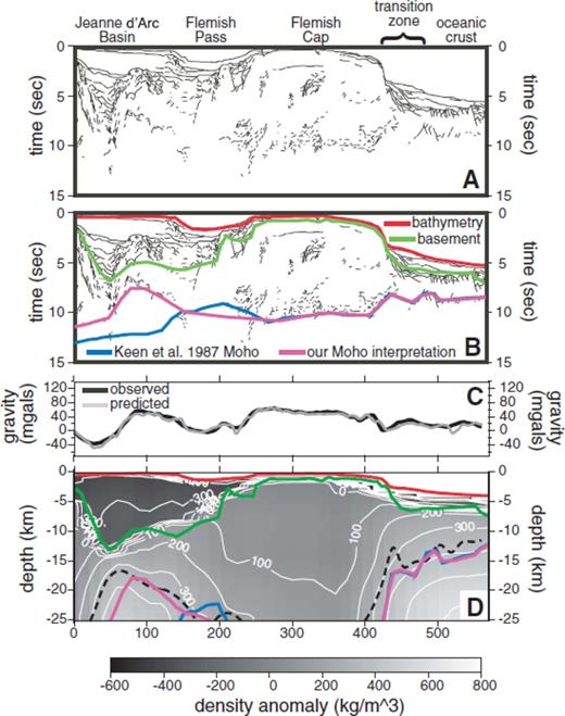
(a) Line drawing interpretation in time of seismic reflection profile F85-3 reproduced from Keen et al. (1987a). (B) Same plot as (A) overlain with time horizons for bathymetry (red line), base of sediments (green line), Moho interpreted by Keen et al. (1987a) (blue line) and our qualitative re-interpretation of the Moho from the reflection section (purple line). (C) Comparison along profile F85-3 of the observed free air gravity anomaly (black line) and the anomaly predicted for the inverted density anomaly model (grey line). (D) Slice through the inverted density anomaly model along profile F85-3 overlain by the Moho depth from Fig. 4(C) (dashed black line) and the depth-converted horizons from (B). The relevant regional features of the margin are labelled along the top of plot (A).
4.4.2 Density variations in the crust and uppermost mantle
In addition to providing Moho constraints, the 3-D gravity inversion results provide information about density variations in the crust and uppermost mantle. These variations can expose lateral changes in crustal structure which may be of tectonic significance. For the purposes of this manuscript, we will loosely define upper crust as corresponding to density anomaly values of less than 100 kg m−3, middle crust as corresponding to density anomaly values between 100 and 200 kg m−3 and lower crust as corresponding to density anomaly values between 200 and 350 kg m−3. These approximate divisions are intended to simplify description of the crustal density variations and aid in their interpretation. We will first describe crustal density variations along the density anomaly model slices shown in Fig. 5 as these correspond to the locations of complementary velocity structural models from seismic refraction profiling.
Profile F84-3, which crosses from the continental shelf onto the thinned continental crust of the Orphan Basin, exhibits a stratified density structure with considerable lateral variations in thickness. At the southwestern end of the profile, crustal density anomalies are generally low with upper-crustal densities occupying most of the crust down to at least 25 km. While these results differ from the colocated seismic refraction results of Chian et al. (2001), who limit upper-crustal velocities to the top 5 km of the crust and model lower crustal velocities between 15 and 36 km depth, the resolved velocities are less constrained than the density values due to the limited seismic ray path coverage at the end of the profile. Off the shelf and into Orphan Basin, the abrupt shallowing of the Moho, which has been interpreted by Chian et al. (2001) as corresponding to a failed rift, is accompanied by a thinned crust dominated by lower crustal high densities. These high crustal densities, which are required by the gravity inversion to compensate for the significant thickness of overlying low density sediments and generate the strong positive anomaly (Fig. 6), agree well with the high lower crustal velocities interpreted at this location by Chian et al. (2001). Beyond the failed rift, the crust beneath the Orphan Basin thickens and appears to be more equally divided between upper-, middle- and lower-crustal densities. A similar division is observed in the seismic refraction results. Finally, at the northeastern limit of the density profile, both upper- and middle-crustal densities are pinched out as the crust thins to less than 10 km and is dominated by higher densities and velocities.
Density variations in the crust and uppermost mantle along the three SCREECH profiles (S1, S2 and S3) are generally quite similar. The slices through the continental shelf of the Flemish Cap for S1 and of the Grand Banks for S2 and S3 all show upper- to middle-crustal density anomalies uniformly dominating within at least the top 15–25 km of the crust. Eastward along the profiles, these lower density anomaly layers are pinched out across the continental slope and towards the higher density oceanic crust beyond. For profile S1, the 100 kg m−3 contour roughly corresponds to the boundary between middle and lower crust resolved from seismic refraction profiling (Funck et al. 2003), implying that the middle crust of the Flemish Cap is of lower density than expected for continental mid-crust. Meanwhile, the continental shelf along profile S3 is uniformly low density down to at least 25 km depth which is consistent with the depth extent of middle crustal material interpreted from the seismic refraction results (Lau et al. 2006a). As with profile S1, the middle crustal material along S3 is of lower density than expected. In contrast to the other SCREECH profiles, lower crustal densities occur at the shallowest level along profile S2. These higher densities may correspond with the lower crustal gabbros interpreted by van Avendonk et al. (2006).
Further south on the tail of the Grand Banks, both profiles F85-2 and F87-5 sample continental crust corresponding to the African Meguma terrane. Not too surprisingly, both profiles exhibit similar density variations for the continental shelf with upper-crustal densities extending to 15 km depth and middle crustal densities extending to at least 25 km. Seismic refraction results along F85-2 show a similarly thick middle crust (Reid 1994). Off the continental shelf, density variations in the crust and uppermost mantle along F85-2 resemble those for the SCREECH profiles further north along the rifted margin while the crustal density distribution along F87-5 thins abruptly across the southern Newfoundland transform margin, becoming dominated by middle to lower crustal densities. This drastic change along profile F87-5 is consistent with the juxtaposition of thick continental crust and thin oceanic crust across a purely transform margin confirmed by earlier seismic refraction results (Todd et al. 1988).
The density anomaly slices in Fig. 7 display a range of crustal density variations. Nearest to land and to the north and east of St. John's, profiles L91-2 and F84-2 are dominated by upper-crustal densities down to at least 25 km depth. At the northeastern limit of the Orphan Basin, the thinner crust of profile F87-4 contains higher densities more akin to oceanic rocks. Towards the northern Grand Banks (F87-1 and F87-2 in Fig. 7), the density anomaly slices display a chaotic distribution of upper- and middle-crustal densities while further south, profile F85-1, which crosses from the Avalon terrane to the Meguma terrane, is more stratified with upper-crustal densities above 15 km depth and middle crustal densities below. Not too surprisingly, profile F85-4 which lies subparallel to profile S3 displays a remarkably similar crustal density distribution.
As with Moho constraints, profile F85-3 again provides one of the most interesting crustal density anomaly distributions of the whole margin. Beneath the Jeanne d'Arc sedimentary basin, the thinned crust is dominated by very high lower crustal densities, possibly suggesting a mafic source. Further northeast, the Flemish Cap is dominated by upper-crustal densities down to 15 km depth at its core but these low densities are pinched out beneath Flemish Pass and towards the Jeanne d'Arc Basin. This drastic contrast may point to a complete separation of Flemish Cap from the rest of the Grand Banks at upper-crustal levels earlier in its history. At its northeastern extent, profile F85-3 displays a thicker crust than profile S1, dominated by lower crustal densities.
5 Discussion
The 3-D density anomaly model derived from the gravity inversion provides an alternate view of the Newfoundland margin that complements existing seismic data sets and can provide further insight into the evolution of the margin. Combining the depth to basement constraints (Fig. 1B) with the hybrid Moho depth model obtained by combining the density results with deep seismic constraints (Fig. 4C), we are able to generate a map of crustal basement thickness across the margin (Fig. 10A). The unique perspective provided by this map allows for an improved discussion of individual components of the margin within a larger context and provides a starting model for reconstructing the 3-D evolution of the rifted margin.
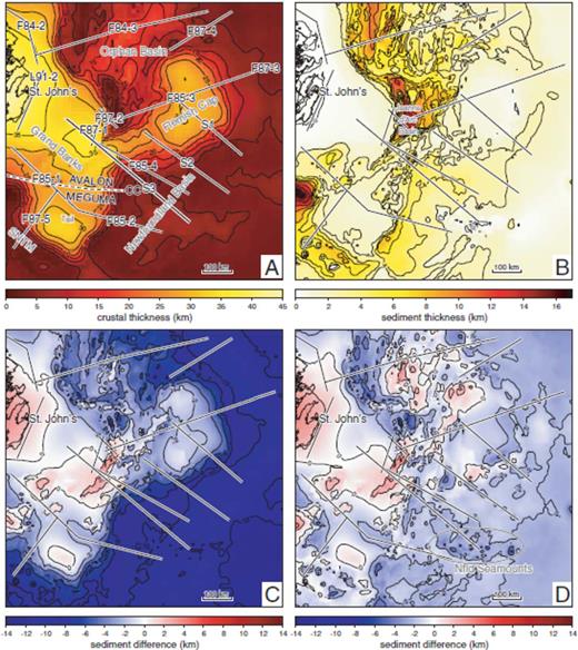
Maps of (A) crustal basement thickness computed from depth to basement (Fig. 1B) and our interpreted Moho depth surface (Fig. 4C), (B) sediment thickness, (C) the difference between the observed sediment thickness for a given crustal thickness and the expected sediment thickness for the isostatically compensated crust in Fig. 11, and (D) the sediment thickness difference in (C) after water depth compensation. The locations of deep seismic profiles acquired over the margin are indicated with black lines outlined in white. In (A), line labels correspond to those plotted in Fig. 1A, key bathymetric structures of the margin are labelled in grey and the Cobequid-Chedabucto Fault (labelled CC), which marks the division between the Avalon and the Meguma terranes, is plotted as the thick black dashed line outlined in white. The location of the Jeanne d'Arc Basin is shown on plot (B). The Newfoundland Seamounts are highlighted with the grey ellipse on plot (D). Abbreviation: SNTM, southern Newfoundland transform margin.
5.1 Grand Banks and Flemish Cap
Just as they dominate the bathymetric map of the Newfoundland margin (Fig. 1A), the Grand Banks and Flemish Cap stand out as the thickest parts of the offshore crust (Fig. 10A). While now separated by the thinner crust south of Orphan Basin, Flemish Cap and the bulk of the Grand Banks have a similar origin as part of the Avalon terrane. Meanwhile, the tail of the Grand Banks originated in Africa as the Meguma terrane (Haworth & Keen 1979). The east-west Cobequid-Chedabucto Fault that marks the boundary between the Avalon and Meguma terranes in Nova Scotia can be extrapolated to the east and is perhaps evidenced by the thinning of the Grand Banks crust north of the tail in Fig. 10(A). The extension of this transform fault into the Newfoundland Basin followed by a change in rifting direction has been proposed as the source of the leaky volcanism that generated the Newfoundland Seamounts (highlighted in Fig. 10D) (Haworth & Keen 1979).
The density anomaly variations within the continental crust of the Grand Banks show regional patterns that can be correlated with their constituent basement terranes. Upper-crustal densities clearly dominate down to at least 25 km depth in the crust from the Avalon terrane (L91-2, F84-2, F85-4, F87-1, F87-2 and S3) while crust from the Meguma terrane shows greater stratification within the top 25 km (F85-1, F85-2 and F87-5). Curiously, the crustal density variations in the Flemish Cap slices (F85-3, S1 and S2) bear a greater resemblance to those from the Meguma terrane than to those from the Avalon terrane, perhaps supporting the notion that the Flemish Cap is a more easterly African terrane with no known exposures above sea level (Enachescu 1992). However, such a conclusion is contrary to palaeoreconstructions which have suggested that Flemish Cap was rotated as a whole in a clockwise direction 43° out of Orphan Basin during the Late Triassic-Early Tertiary and was further translated 200–300 km southeastward (Srivastava & Verhoef 1992; Enachescu 2006; Sibuet et al. 2007).
5.2 Orphan Basin
North of the Grand Banks, the Orphan Basin represents a broad region of extended continental crust, generally ranging in thickness from 5 to 15 km. Just as with Flemish Cap and the bulk of the Grand Banks, the continental crust of the Orphan Basin originated as part of the Avalon terrane. However, closely spaced faults within the basin experienced much greater extension than those on the Grand Banks to the south. The northwest boundary of the basin corresponds to the transform margin of the Charlie Fracture Zone while its southeastern boundary with Flemish Cap has also been interpreted as a transform margin, the Cumberland Belt Fault Zone (Enachescu 2006).
The density anomaly variations across the Orphan Basin show a very different structure to that of the less extended Avalon basement of the Grand Banks. Along profile F84-3 in Fig. 5, only a thin layer of upper-crustal densities is observed at the centre of the basin and this is pinched out completely above the inferred failed rift to the west (Chian et al. 2001). This pinching out of the upper-crustal layer is similar to that observed to the west of Flemish Cap on profile F85-3 (Fig. 7). From the areal distribution of thinned crust across the western Orphan Basin (Fig. 10A), profiles F84-3 and F85-3 may both be sampling an extensive NW—SE oriented failed rift system.
The interpreted failed rift along profile F84-3 is believed to have been generated during a period of major extension that began 100 km to the south in the Jeanne d'Arc Basin in the mid-Jurassic (160 Ma) and progressed into the West Orphan Basin during the Cretaceous (Chian et al. 2001). The shallow Moho observed to the west of Flemish Cap along profile F85-3 may represent an earlier phase in this same extensional episode. This period of rifting is thought to have continued until late Cretaceous when rifting jumped outboard by 200 km and the Labrador Sea was initiated between Canada and Europe (Haworth & Keen 1979).
Along this interpreted failed rift in the southwestern Orphan Basin where the sedimentary basins are 12–14 km deep and the crust is thin and on the order of 5–10 km (or slightly less if we limit the maximum density anomaly used for the sediments in the inversion to −200 kg m−3), the presence of anomalously high gravity signals implies that the sedimentary basins are not entirely compensated isostatically and that the underlying lithosphere retains some rigididity, despite having undergone significant local extension (Chian et al. 2001). While rupturing of the crust along profile F84-3 can be ruled out based on the continuity of continental crust, seismic refraction/wide-angle reflection profiling would be required along profile F85-3 and to the northwest to determine whether the crust remained intact across the entire interpreted failed rift or whether separation did occur to the west of Flemish Cap. With enhanced seismic coverage, the influence on the failed rift of the rotation and translation of Flemish Cap out of Orphan Basin and the associated shear zone along the SW margin of Flemish Cap could be investigated (Sibuet et al. 2007).
5.3 Sediment excess and deficiency on the margin

Assuming that the crust was 36 km thick before thinning and that ρs, ρc and ρm are 2200, 2850 and 3300 kg m−3, respectively, we obtain the relationship between sediment and crustal thickness plotted as the thick black line in Fig. 11. From further plotting of the sediment versus crustal thicknesses for all locations in our study area as grey crosses, it becomes evident that the sediments of the Newfoundland margin are generally not as thick as would be predicted assuming isostatic compensation. While this may simply reflect our choice of density values, this choice does not greatly bias the results as illustrated by the two grey lines in Fig. 11 which correspond to the derived sediment/crustal thickness relationship assuming a sediment density of 2100 kg m−3 (lower line) and 2300 kg m−3 (upper line)

Plot of crustal basement thickness versus sediment thickness (grey crosses) for all locations in the survey area. The black line denotes the isostatically compensated trade-off between sediment and crustal thickness assuming that sediment free crust should be 36 km thick and the densities for sediments, crust and mantle are 2200, 2850 and 3300 kg m−3, respectively. The two grey lines show how the trade-off would change for a sediment thickness of 2100 kg m−3 (lower line) and 2300 kg m−3 (upper line). The black arrow shows how the sediment differences in Fig. 10(C) were calculated for a given sediment/crust thickness combination.

Our choice of sediment density results in modest overcompensation in deep water, but the value of the approach is in the ability to identify strong gradient zones. Such gradient zones can be useful in identifying dominant listric detachments (Fig. 12). To illustrate this, suppose the crust is extended by a listric normal fault and the accommodation space is filled with sediments (grey shading, Fig. 12A). The isostatic response, given finite flexural rigidity of the lithosphere, results in a broad uplift over the basin and its margins (Fig. 12B). Erosion of the uplifted area might result in the final configuration shown in Fig. 12(C). In Fig. 12(D), the changes in sedimentary thickness are compared with those of crustal thickness for a locally compensated Airy isostatic model, to reveal where these are out of balance in the final configuration. Approaching the basin from the left, crustal thickness starts to decrease, but there are no sediments until the outcrop of the listric fault is reached. So, this area is one of sediment deficit (in the local Airy assumption). This situation changes rapidly crossing the basin so that an area of sediment excess is revealed. There is then another area of sediment deficit beyond the basin at the right end of the model. Thus, finite flexural rigidity in a simple shear extension produces areas of sediment deficit and excess that are geographically localized by a degree related to the flexural rigidity, but that are balanced out on a wider regional basis. Consequently, steep listric faults are revealed as strong gradient zones in the sediment thickness excess/deficit map (Fig. 10D).
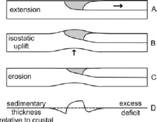
Cartoon showing how simple-shear extension along a listric detachment and consequent sedimentary basin formation (A), in a lithosphere with flexural strength, leads to isostatically driven distributed uplift (B), erosion (C) and a corresponding variation of sedimentary thickness (relative to crustal thickness, (D) from that expected for local Airy compensation. Note the high gradient over the basin edge where the detachment surfaces. The high gradient over the basement downlap in the hangingwall will be lower in amplitude if the angle of downlap is reduced by terminal drag.
The superposition of known basin geology on the sediment thickness excess/deficit map confirms this relationship (Fig. 13). The Murre Fault is the major normal fault bounding the WNW-side of the Jeanne d'Arc basin, and has been interpreted as a listric detachment soling deep in the crust (Enachescu 1992). Its course clearly follows a strong gradient in excess sediment thickness, with the excess increasing on the basin side. Many other features of the map correlate with known geological features (Fig. 13). In the Orphan basin, three of the major faults, the Bonavista, Flying Foam and White Sail Faults, all run close to parallel with the deficit and excess sediment contours. The division into an early (Triassic—Jurassic) east Orphan basin and a later (Cretaceous) west Orphan basin at the White Sail fault (Enachescu 2006) is no more obvious in the map trends than the Flying Foam Fault. As such, we would argue that distributed listric faulting has instead spread the extension (as it is measured in total today) across a series of faults. The Carson and Bonnition basins at the edge of the SE Newfoundland basin correlate with weakly defined gradient zones running in around the basins' edges, defined by faults (Solvason 2006). The north—south trending grabens (Anson, Flemish Cap and southern part of Flemish Pass) also follow the map trends. Interestingly, the northern part of the Flemish Pass basin lies along a NNE—SSW-trend in the excess sediment map, and the N—S trends of the graben faults cut across this. We infer that the Jeanne d'Arc, Carson, Bonnition and Flemish Pass basins originated as NNE—SSW trending rifts, reflecting early (Triassic—Jurassic) NW—SE extension that began the opening of the Atlantic in the SE Newfoundland basin. As rifting and seafloor spreading shifted northwards, the direction of extension rotated anticlockwise to east—west (and later NE—SW) but this had more effect on the outboard basins farther north (Anson, Flemish Cap and Flemish Pass grabens). As a consequence, the Flemish Pass basin retains a NNE—SSW trend from its early history but the later faults dissect it in a N—S direction.
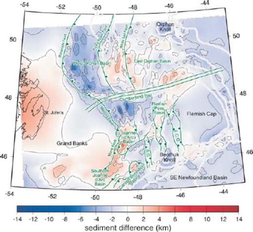
Enlarged portion of the map in Fig. 10(D) of sediment thickness difference after water depth compensation. The main faults are shown as green lines and labelled in green. The light grey lines represent the 1, 2, 3 and 4 km bathymetric contours (compare against Fig. 1A). Key bathymetric structures of the margin are labelled in black. Abbreviations: F.C.G., Flemish Cap Graben; A.G., Anson Graben.
The continental shelf edge is not conspicuous on Fig. 13: it corresponds to a poorly defined region without a characteristic variation in sediment deficiency or excess. However, the SSE margin of Flemish Cap shows a slight gradient. This gradient may be caused by listric faulting associated with the rifting of this side of the Flemish Cap, with the gradient perhaps accentuated by the very rapid continent—ocean transition in this area (Todd & Reid 1989; Funck et al. 2003). There is continuing debate about whether this is a regular extended margin, an obliquely formed margin with significant transform motion (Todd & Reid 1989), or some compounding of these related to clockwise rotation of Flemish Cap from out of Orphan basin (Srivastava & Verhoef 1992; Enachescu 2006; Sibuet et al. 2007). Regional palinspastic restorations are needed to resolve this issue. If the margin were simply transform (continent—ocean), then there would be a complex thermal history for this edge of Flemish Cap. As the northern limit of the new-born spreading centre migrated along the transform, there would be a diachronous lateral heating and subsequent cooling of the continental edge of Flemish Cap to the north of the fault. As the flexural rigidity changed in response to the heating and cooling, it would be difficult to model the exact response of the Cap, although one would expect some noticeable change in sediment and/or crustal thickness along the margin, which is not readily observed. Post-spreading thermal subsidence on the ocean side might be expected to lead to a downward drag on the Cap rather than the uplift and subsequent erosion that would result from a seaward-dipping listric detachment.
In Fig. 13, circular lows correspond with local bathymetric highs (Orphan and Beothuk Knolls) suggesting that both are buoyed up to some degree by adjacent lithosphere. The large gravity high north of the Jeanne d'Arc basin shows as a deep low in the sediment excess map. It has internal structure indicating NNW—SSE-controlling faults which may well connect with faults of this trend in the southern parts of Orphan basin across the intervening Cumberland Belt. While the Cumberland Belt has been identified as a major transfer zone, Jurassic-aged sediment-filled troughs have been seen to connect across the belt (Enachescu 2006), undermining its significance.
5.4 Towards a new palaeoreconstruction of the margin
Existing palaeoreconstructions of the Newfoundland margin and its conjugates have primarily involved the matching up of the margins along progressively older magnetic lineaments (Verhoef & Srivastava 1989). While tremendously informative, these reconstructions have generally treated the margins themselves as static building blocks without consideration of deformation and reorganization within the margins. A preliminary attempt at extending beyond the classic reconstructions has been undertaken by Srivastava & Verhoef (1992) who have investigated the progressive development of Mesozoic sedimentary basins of the North Atlantic. Their results have helped shed light on reorganizations within the Newfoundland margin such as the rotation of Flemish Cap and the opening of individual basins. Still, and in light of the results presented in this manuscript, many questions remain and the next generation of palaeoreconstructions is now needed to both satisfy the overall magnetic constraints and the regional dynamics within the individual margins.
Our results from the gravity inversion have highlighted a number of intriguing features. Most striking is the extreme shallowing of the Moho to 12 km immediately to the north of the Jeanne d'Arc basin. If this shallowing represents a failed rift which connects to the one inferred in the south of the West Orphan Basin by Chian et al. (2001), then this is a massive feature, previously unrecognized, that must be worked into the reconstruction.
The Flemish Cap remains an enigmatic feature, both in terms of the nature of its boundaries and also its relation to the rest of the Grand Banks. The crustal density anomalies point to a complete separation of the upper crust of Flemish Cap from the rest of the margin, possibly during the development of the failed rift.
Finally, in the case of both Flemish Pass and the Orphan Basin, the sediment excess map (Fig. 13) appears to highlight ancient structures that have been overprinted by more recent faulting. This preservation of old trends may prove tremendously useful for future more detailed reconstructions. Future gravity inversions over the conjugate margins may help further the piecing together of the rifted margins.
6 Conclusions
We have undertaken 3-D gravity inversion of the free air data over the Newfoundland margin and generated a regional density anomaly model that satisfies constraints obtained by seismic methods. A hybrid Moho map for the margin based on the gravity inversion and deep seismic results offers a unique view of the margin. In particular, a shallowing of the Moho to 12 km depth to the north of Jeanne d'Arc Basin represents a previously unrecognized feature that may form part of an extensive failed rift along the southern margin of the Orphan Basin. Isostatic compensation is investigated across the margin by comparing crustal and sediment thicknesses. Sediment thickness deviations from those expected for a compensated crust help highlight listric detachments in the crust even when they have been overprinted by younger structures. In all, the results provide a unique perspective of the margin and present further constraints for future palaeoreconstructions.
Acknowledgments
We would like to thank Sonya Dehler and Christel Tiberi for carefully reviewing this manuscript and providing excellent constructive criticism. We would also like to thank the Atlantic Innovation Fund for its support of the PanAtlantic Petroleum Systems Consortium (PPSC) which contributed to postdoctoral salary support; Sonya Dehler from the Geological Survey of Canada for providing the appropriate datasets; and the Natural Sciences and Engineering Research Council of Canada for funding in support of this research (Discovery Grant to Hall).
References
