Radial resolving power of far-field differential sea-level highstands in the inference of mantle viscosity Free

Summary

1 Introduction

The detailed depth variation of viscosity in the Earth's mantle remains a contentious issue. Analyses of observables related to mantle convection, such as long-wavelength geoid anomalies, have consistently preferred a mantle viscosity that increases by more than an order of magnitude from the upper to the lower mantle (e.g. Hager 1984; Ricard et al. 1984; Richards & Hager 1984; Forte & Peltier 1991; King & Masters 1992). However, viscosity profiles inferred from geophysical observables associated with glacial isostatic adjustment (GIA) have been characterized by less consensus.

McConnell (1968) derived the Fennoscandian Relaxation Spectrum (i.e. decay time of strandline uplift versus spatial wavelength) for a plane Earth and inferred a significant, factor of ∼25, increase of viscosity from the upper mantle to the top portion of the lower mantle. In contrast, the first global, spherical Earth analyses of GIA data argued for an essentially isoviscous mantle, or, at most, a moderate (factor of ∼2) increase of viscosity from the base of the lithosphere to the core—mantle boundary (CMB) (Cathles 1975; Peltier & Andrews 1976). Subsequent studies by Peltier and colleagues (e.g. Wu & Peltier 1983, 1984; Tushingham & Peltier 1991), based on relative sea level (RSL) and anomalies in rotation and gravity, further supported this conclusion, and this led to arguments that transient effects (i.e. timescale dependence) in viscosity were required to reconcile the disparate inferences from convection and GIA data (e.g. Peltier 1985; Sabadini et al. 1985; Peltier et al. 1986; Yuen et al. 1986). However, the prevailing view of an isoviscous mantle on GIA timescales was countered by the GIA-based analysis of Nakada & Lambeck (1989) and Lambeck & Nakada (1990) (henceforth the NL studies), who argued for an approximately two order of magnitude increase in viscosity from the upper to lower mantle.

A complication in inferring mantle viscosity from GIA data is that the raw observables are sensitive to uncertainties in the space—time geometry of the Late Pleistocene ice loads. To limit this sensitivity, the NL analyses were based on the differential amplitude of sea-level highstands recorded in the Australian region. In this area, RSL variations subsequent to the last glacial maximum are generally characterized by a rapid sea-level rise during the deglaciation phase, followed, in the last 4–6 kyr, by a gradual decrease extending to the present-day. Although the ensuing highstand amplitudes are relatively insensitive to the geographical distribution of the former ice loads, they are sensitive to remnant melting following the primary phase of deglaciation. This sensitivity can be significantly reduced by considering the difference in highstand amplitudes between two relatively nearby sites (we use the notation DSL to refer to these differential sea-level highstands). Using a set of such DSL data, NL inferred an elastic lithospheric thickness (LT) in the range 70–80 km, an upper mantle viscosity (ν_um) of 2 − 3 × 10²⁰ Pa s, and a lower mantle viscosity (ν_lm) of ∼10²² Pa s.

Nakada & Lambeck (1991) compared this result with inferences they derived from sea-level data sets in other regions, including Hudson Bay, Northwestern Europe and Pacific islands. The Pacific island data suggested an upper mantle viscosity less than 10²⁰ Pa s, while the remaining three data sets preferred ν_um∼ 3 × 10²⁰ Pa s. In contrast, these three data sets were best fit by lower mantle viscosities ranging from 4 × 10²¹ Pa s for Europe (in agreement with later work by Lambeck et al. 1998) to 3 × 10²² Pa s for Hudson Bay. This variation led them to argue for the presence of lateral heterogeneity in mantle viscosity.

The robustness of such an argument is complicated by several factors. First, with the exception of the DSL data from Australia, the remaining data sets involved raw RSL histories, and were thus sensitive to the adopted surface loading history. Second, these inferences were all based on simple three parameter (LT, ν_um, ν_lm) forward analyses, and thus they do not provide a measure of the detailed depth dependence on viscosity of the various data sets. This dependence must be unique given the distinct spatial scales associated with the ice loading over Fennoscandia and Laurentia and the ocean loading at Australian coastal and Pacific island sites. Thus, the differences cited above may reflect a limitation of the forward model parametrization rather than necessarily reflecting lateral rheological structure.

To assess the radial resolving power of GIA data sets requires the application of formal geophysical inversion procedures. To date, such inversions have focused largely on decay times derived from postglacial emergence curves. The uplift of previously glaciated regions is characterized by (relatively) free decay, and the associated RSL curves may be accurately described by a simple exponential form (Andrews 1970; Walcott 1980). Whereas the amplitude of this form is a function of the local ice load thickness, the decay time is relatively insensitive to the finer details of the load history, and Mitrovica & Peltier (1993) have thus advocated their use in constraining the radial profile of mantle viscosity. As an example, Mitrovica (1996) analysed the postglacial decay time of Angermanland in central Fennoscandia to revisit the classic Haskell (1935) constraint on mantle viscosity (10²¹ Pa s). He demonstrated that previous inferences of an isoviscous mantle (e.g. Tushingham & Peltier 1991) were biased by a misinterpretation of the Haskell average as a constraint on the mean upper mantle viscosity; a resolving power analysis indicated that the true average extended to ∼1400 km depth. Moreover, joint, multilayer inversions of a suite of mantle convection data and GIA observables, including decay times from Fennoscandia, Hudson Bay (where resolving kernels extend from ∼400 to 1800 km depth; Mitrovica & Forte 1997) and a revised Fennoscandian Relaxation Spectrum (Mitrovica & Forte 2004), indicate that both classes of data may be simultaneously reconciled by a viscosity profile characterized by a significant increase with depth. Specifically, the most recent inference involved a three order of magnitude increase from the upper mantle (∼4 × 10²⁰ Pa s) to the top of the lower mantle (∼2 × 10²¹ Pa s) and a high viscosity peak (10²³ Pa s) at 2000 km depth. A similar reconciliation of GIA and convection data sets was reported by Kaufmann & Lambeck (2000).

The main objective of the present paper is to revisit the influential analysis of NL within the framework of (Bayesian) inverse theory. Specifically, our goal will be to provide the first formal assessment of the radial resolving power of the DSL data set; that is, to identify the specific radial averages of mantle viscosity that are resolved by the far-field data. Given the specific aim of the present study, our analysis follows as closely as possible the original NL study. In particular, we will use the same site pairs to define the DSL data. Moreover, the global ice load we adopt will be very similar to the model constructed by NL. One notable change from the earlier studies will be the theory we adopt for predicting postglacial RSL variations. Since the early 1990s there have been significant improvements in this theory [see Mitrovica & Milne (2003) for a recent review], and we are compelled here to adopt these improvements.

To begin, we summarize those parts of the analysis procedure that are distinct from NL, in particular, the Bayesian inversion algorithm and the new aspects of the sea-level theory. We note that the former includes parameters for both mantle viscosity and lithospheric thickness. Next, we establish the resolving power of the DSL data adopted by NL using a set of synthetic data inversions.

2 Theory

2.1 The generalized sea-level equation

We solve the generalized sea-level equation developed in Mitrovica & Milne (2003) using the numerical algorithm derived in Kendall et al. (2005). This equation extends the traditional GIA theory of Farrell & Clark (1976) to accurately account for time dependence in shoreline geometry arising from local transgression and regression of water or changes in grounded marine-based ice.

Sea level, SL(θ, ψ, t), where θ and ψ are the colatitude and longitude and t is time, is defined globally as the difference between the geoid and the solid surface. The ocean height or bathymetry, S(θ, ψ, t), is the projection of the sea level onto the ice-free oceans. The location of the ice-free oceans is represented by the ocean function C(θ, ψ, t)=1, whereas C(θ, ψ, t) = 0 over both land and regions where marine ice is grounded. If we denote the change in sea level from the onset of loading (t₀) to an arbitrary time t as ΔSL(θ, ψ, t), then the change in the ocean height can be computed from (Mitrovica & Milne 2003)

1

This equation is an integral equation since the field ΔSL(θ, ψ, t) is computed as a response to the total surface mass load which is comprised, in part, of the ocean height change ΔS(θ, ψ, t). Moreover, the time-dependent field C(θ, ψ, t) is also a function of the ocean load. The sea level at time t relative to that at present, t_p, or relative sea level, at a specific site (θ_m, ψ_m) can be written as

2

Although the generalized eq. (1) holds for any type of earth model, our calculations assume spherical symmetry and are based on the extended pseudo-spectral technique described by Kendall et al. (2005) for this special case. In this regard, we adopt a truncation at spherical harmonic degree and order 128. Predictions of the change in sea level require a formalism for computing the deformational and gravitational response to the surface mass load. For this purpose we adopt Maxwell viscoelastic Love number theory (Peltier 1974). The elastic and density structure of the earth model is given by the seismically determined PREM (Dziewonski & Anderson 1981). We have reconstructed an ice load history that is similar to the ARC3+ANT3 ice history of Nakada & Lambeck (1988).

An example of a forward prediction for four sites in the Australian region is shown in Fig. 1. (The location of these sites, and others included in the analysis below, is given in Fig. 2.) The predicted highstands at 6 kyr bp coincide with the end of the deglaciation phase in the ARC3+ANT3 history. The sea-level curves show a dramatic rise in consequence of the meltwater flux during the main deglaciation phase. Subsequently, the curves tend to exhibit a small decrease to the present-day which yields a characteristic sea-level highstand. The sea-level fall during the interglacial is driven by the combined effects of processes known as ocean syphoning and continental levering (for a recent review, see Mitrovica & Milne 2002). Ocean syphoning describes the fall in far-field sea level resulting from the movement of water from the far-field to the near-field as the peripheral bulge subsides. Continental levering refers to the tilting of continents due to the differential loading across the continental margin.

Figure 1.

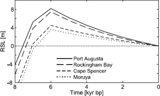
Forward predictions showing typical RSL highstands at four sites in Australia.

Open in new tabDownload slide

Figure 2.

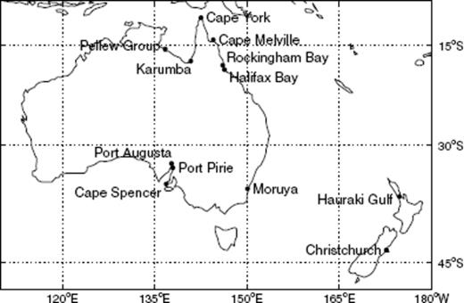
Location of sites at which synthetic RSL highstands are computed.

Open in new tabDownload slide

As discussed in the Introduction, RSL predictions will be sensitive to remnant melt (i.e. melt persisting beyond the main deglaciation phase), and thus NL introduced the notion of differential sea-level highstands (DSL). For two nearby sites m and n, the DSL may be written as

3

where t_e corresponds to the time of maximum emergence, or timing of the highstand.

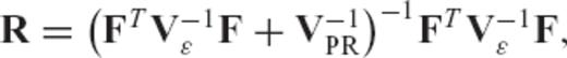
2.2 Bayesian inversion

Let a set of observables y, and their associated errors e, be related to the true model, x, by the following non-linear relation,

4

In our analysis, the observable y_i will be the DSL highstand for site pair i, that is

5

The unknown rheological model x is comprised of two sets of parameters. The first is the logarithm of viscosity as a function of depth. We discretize this profile using 21 layers in the lower mantle and 13 layers in the upper mantle, where the boundary between the two is at 670 km depth. The second component of the model x is the thickness of an elastic lithosphere. Thus, we perform a simultaneous inversion for both viscosity and lithospheric thickness. NL have shown that forward predictions are sensitive to the lithospheric thickness, and thus the inclusion of this parameter is important to avoid biasing inferences of viscosity.

We solve for x in eq. (4) using a non-linear Bayesian formulation (Jackson 1979; Backus 1988), which provides an algorithm for combining a priori information on the earth model (for example, the lithospheric thickness may be limited to values consistent with those inferred from previous GIA studies) with observational constraints. Following Tarantola & Valette (1982), we use an iterative equation of the form,

6

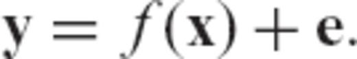
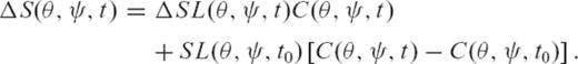
where denotes the kth iterate estimate of the earth model vector, F_k is the matrix of Fréchet kernels computed using this solution, x_PR and V_PR are prior model and covariance matrices, y and V_ɛ denote the observed data and covariance (error) matrix, and is the non-linear forward prediction (see Section 2.1) based on the estimate .

Fréchet kernels relate arbitrary perturbations in the model parameters to perturbations in (forward predictions of) the observables. For simultaneous inversions of the viscosity, ν(r), and the lithospheric thickness, LT, the Fréchet kernels have two parts. The first is associated with a perturbation in the viscosity profile, and may be defined by

7

where FK_i is the Fréchet kernel for the ith datum (i.e. the ith row of matrix F), and r_lt is the radius at the base of the elastic lithosphere. Note that the radius r in eq. (7) has been normalized by the radius of the Earth, a. The second component of the Fréchet kernel is associated with the perturbation in the lithospheric thickness, and may be defined by

8

The dependence of the kernels on ν(r) and LT makes explicit the non-linear nature of the forward problem. The kernels for a given earth model are computed numerically by perturbing, individually, the value of the lithospheric thickness and the viscosity within each of the 34 mantle layers.

The resolving power of the data can be assessed by examining the posterior covariance matrix. Our adoption of a logarithmic parametrization of mantle viscosity weakens the non-linearity of the inverse problem (Mitrovica & Peltier 1991a) and improves the stability of the above iterative scheme. For such weakly non-linear problems, the posterior covariance matrix can be approximated by (Tarantola & Valette 1982; Jackson & Matsu'ura 1985)

9

where F is computed from the posterior model. Each row of the covariance matrix corresponds to a different target depth and the diagonal elements represent the variances for the individual model estimates. The pattern of covariances along any particular row reflects the resolving power of the data at the corresponding target depth. For example, one can use the spread of these covariances as a measure of the resolving power.

Following Jackson (1979), we will also be interested in comparing the prior and posterior variances of averages of the model parameters through the ratio

10

For small values of S², the general linear combination g^Tx is deemed well resolved by the data. We choose g such that g^Tx is the volumetric average (over a radial width we will denote by w) of the logarithm of viscosity.

3 Results

We begin by presenting Fréchet kernels for sea-level highstands computed using a model close to that preferred by NL. These kernels provide a measure of the detailed sensitivity of the data to depth-dependent variations in mantle viscosity and changes in the elastic thickness of the lithosphere. Next, we perform a set of inversions using synthetic (i.e. numerically derived) DSL values for the 14 site pairs adopted by NL and listed in Table 1. The first such inversion is based on a prior constraint of a two-layered viscosity model. We next extend this simple case to consider a multilayered viscosity profile and examine the detailed resolving power of the synthetic data. These inversions are performed with and without observational errors applied to the synthetic data. The locations of the sites that define the DSL highstands are given in Fig. 2.

Table 1.

Contributions to change δDSL [m] (eqs 8 and 11) resulting from the perturbation to the parameter listed in the subscript. δDSL_lm and δDSL_um were computed for a uniform perturbation δlog ν = 0.3, and δDSL_lt was computed for a perturbation δLT = 10 km.

Open in new tabDownload slide

3.1 Fréchet kernels

As discussed in Section 2.1, relative sea-level variations in the far-field are driven by two processes. Ocean syphoning is a long-wavelength effect that is sensitive to the dynamics of the peripheral bulge and is therefore expected to show the same sensitivity to mantle viscosity as the integrated deformational response across the subsiding peripheral bulge. Fréchet kernels for the present-day radial velocity at sites spanning the Laurentian peripheral bulge (frames D, E, F of fig. 12 in Mitrovica et al. 1994) show a sensitivity to viscosity at all depths. Indeed, for sites located on the outer edge of the bulge region, sensitivity to the lower mantle remains nearly constant down to the CMB. Sites spanning the position of maximum subsidence through to the outer flank of the peripheral bulge show a maximum sensitivity to viscosity at depths near the 670 km boundary. We therefore expect the component of far-field RSL resulting from syphoning to exhibit sensitivity to changes in viscosity at all depths within the mantle. Far-field relative sea level is also driven by continental levering. Continental levering can occur on both long-wavelength scales (across whole continents) as well as on a variety of local scales (along peninsulas, for example; Nakada & Lambeck 1989). This is due to the mix of spatial wavelengths that define the ocean load in regions surrounding the continents and islands.

Fréchet kernels for RSL highstands were computed numerically using equations analogous to (7) and (8), where we have used RSL highstands in place of DSL. The computations adopt a lithospheric thickness of 71 km, and constant upper and lower mantle viscosities of 0.5 × 10²¹ and 5 × 10²¹ Pa s. The RSL kernels (Fig. 3) show the greatest sensitivity to viscosity within model layers in the upper mantle, where local levering effects can cause the sensitivity to vary dramatically from site to site. There is also a non-negligible sensitivity to the lower mantle viscosity resulting from the long-wavelength effects mentioned above. This sensitivity shows a similar trend from site to site, and is therefore expected to decrease significantly when DSL highstands are constructed.

Figure 3.

Numerically computed RSL Fréchet kernels for the individual sites considered in this study. The earth model used in the computations is defined by an elastic lithosphere of thickness LT = 71 km, ν_um = 0.5 × 10²¹ Pa s and ν_lm = 5 × 10²¹ Pa s. The vertical dashed line indicates the 670 km depth boundary.

Open in new tabDownload slide

Numerically computed DSL kernels are plotted in Fig. 4 for 12 of the 14 pairs of sites treated by NL (see caption). The sensitivity to variations in viscosity within upper mantle layers resulting from the shorter wavelength signal of local continental levering effects remains large. As with the RSL kernels, this sensitivity can vary greatly between pairs of sites. In contrast, the sensitivity evident in the predicted RSL signal, resulting from processes such as ocean syphoning and long-wavelength ocean-driven continental levering, is partially cancelled by considering the difference in these highstands. Thus, as predicted from the RSL kernels, the sensitivity to the viscosity in lower mantle layers has been significantly reduced, though it has not been eliminated entirely. Notable examples of this sensitivity are the kernels for Rockingham Bay—Moruya and Cape York—Rockingham Bay.

Figure 4.

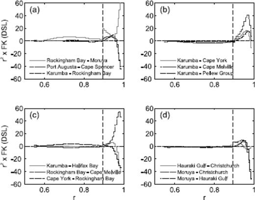
Numerically computed DSL Fréchet kernels for the pairs of sites treated in this study. Note that the kernel for Port Pirie—Cape Spencer is nearly identical to that for Port Augusta—Cape Spencer in (a) and has been omitted from the figure for clarity; similarly, the kernel for Halifax Bay—Moruya is nearly identical to that for Rockingham Bay—Moruya in (a), and has also been omitted. The earth model used in the computations is defined by LT = 71 km, ν_um = 0.5 × 10²¹ Pa s and ν_lm = 5 × 10²¹ Pa s.

Open in new tabDownload slide

The relative insensitivity of the DSL predictions to variations in viscosity within the individual lower mantle layers does not necessarily suggest that the data are more sensitive to bulk changes in the upper versus lower mantle viscosity. To quantify this relative (bulk) sensitivity, consider the case where we apply a uniform (and identical) perturbation to viscosity (δ log ν) within each of these regions of the mantle. In this case, eq. (7) may be used to write

11

where r₆₇₀ is the radius at 670 km depth.

In Table 1, we present the contributions to the total change δDSL based on a uniform perturbation of δlog ν = 0.3 to the upper and lower mantle and the Fréchet kernels in Fig. 4. That is, δDSL_lm is the change in DSL expected from a uniform perturbation of δlog ν = 0.3 (i.e. a factor of two change in viscosity) in the lower mantle, and similarly for δDSL_um. Clearly, the sensitivity of the DSL predictions to bulk variations in the lower mantle viscosity is comparable to a similar variation in upper mantle viscosity at many site pairs.

Previous studies of DSL data have been limited to isoviscous upper and lower mantle regions and, hence, to bulk changes in viscosity within each. The depth-dependent kernels in Fig. 4 indicate that these bulk measures miss important sensitivities at shorter radial scales. Consider, for example, the results in Table 1 for Karumba—Rockingham Bay, which indicate a relatively minor (in comparison to other site pairs) sensitivity to bulk changes in upper mantle viscosity. Examining the sensitivity kernel for this site pair as a function of depth in Fig. 4(a) shows that there is, in fact, a relatively significant sensitivity to variations in viscosity at the base of the lithosphere. However, since the kernel for this DSL prediction changes sign within the upper mantle, partial cancellation occurs when considering the bulk sensitivity.

To complete the analysis of the Fréchet kernels, we also present the results of eq. (8) in Table 1, where, for illustrative purposes, δDSL_lt is listed for a perturbation of δLT = 10 km. (Thus we are comparing, in Table 1, changes in DSL predictions arising from changes in LT of 10 km versus a factor of two increase in either ν_um or ν_lm.) There is considerable variation in the sensitivity to lithospheric thickness between site pairs. In some cases this sensitivity is as expected. For example, Port Augusta and Cape Spencer lie at opposite ends of a long, narrow inlet, and therefore predictions of DSL for this site pair will be sensitive to the influence of the choice of LT on the predicted amplitude of levering (and relatively less sensitive to changes in ν_um and ν_lm; NL). In contrast, the DSL prediction for Rockingham Bay−Cape Melville shows a marked insensitivity to changes in LT, which is likely a consequence of the location of these sites relative to the coastline. These sites lie parallel to the broad, levering-induced tilt of the coast, and thus taking the difference in the RSL predictions to compute the DSL will strongly reduce the sensitivity to LT. (Note that Port Augusta and Cape Spencer lie perpendicular to the tilting.) However, the prediction Rockingham Bay−Cape Melville does show a strong sensitivity to changes in viscosity within the top half of the upper mantle (Fig. 4c).

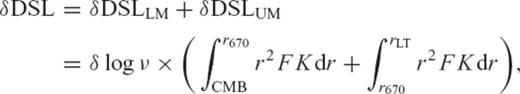
The results presented in Figs 3, 4 and Table 1 were all obtained using the same earth model (LT = 71 km, ν_um = 0.5 × 10²¹ Pa s and ν_lm = 5 × 10²¹ Pa s). Since the predictions (and hence the inversions) are non-linear functions of the earth model, the Fréchet kernels (i.e. the depth sensitivity) for these DSL predictions will also be a function of the earth model. To explore this issue, in Fig. 5 we show kernels computed using a suite of earth models defined by LT = 71 km, ν_um = 0.5 × 10²¹ Pa s and uniform lower mantle viscosities ranging over two orders of magnitude. Fig. 5(a) shows the results for Port Augusta−Cape Spencer. As the viscosity in the lower mantle increases, the sensitivity to the viscosity within the lower mantle tends to decrease. The sensitivity to the transition zone shows a monotonic change as the lower mantle viscosity of the earth model is increased, while the sensitivity to the shallow upper mantle remains high in all cases. In contrast, for Rockingham Bay—Moruya (Fig. 5b) the sensitivity to the lower mantle changes less predictably, and only decreases to near-zero at the highest value of the adopted viscosity within this region. Near the 670 km boundary the change in sensitivity is non-monotonic. Again, the sensitivity to the shallow upper mantle viscosity remains high.

Figure 5.

Numerically computed Fréchet kernels for the DSL highstand of (a) Port Augusta—Cape Spencer and (b) Rockingham Bay—Moruya. The earth model in each of the computations is defined by LT = 71 km, ν_um = 0.5 × 10²¹ Pa s and a lower mantle viscosity as labelled.

Open in new tabDownload slide

3.2 Inversions of synthetic data

To begin, we generate a suite of synthetic DSL highstands, y, using an earth model with a lithospheric thickness of 71 km, and a mantle consisting of constant upper and lower mantle viscosities of 0.5 × 10²¹ and 5 × 10²¹ Pa s. We begin the iterations with a starting model, , defined by LT = 96 km, ν_um = 10²¹ Pa s and ν_lm = 10²² Pa s. Throughout this section, we set the prior model, x_PR, equal to the starting model.

The first inversions are based on a prior assumption of a two-layered viscosity model. To this end, we construct a prior covariance matrix which consists of a high (essentially perfect) correlation between each model layer in the upper and, separately, the lower mantle. That is, the model values are strongly correlated within each of these two mantle layers, but there is zero prior correlation between layers on either side of the 670 km depth boundary. This special case is consistent with the usual assumption in forward modelling of GIA data of isoviscous upper and lower mantle regions. The prior viscosity variances are chosen to be sufficiently weak (we adopt a value of 50, or approximately a ± 7 order of magnitude change) to ensure that the inversions are not influenced by this parameter. Furthermore, the prior variance for the lithospheric thickness is 3600 km² (corresponding to ±60 km standard deviation).

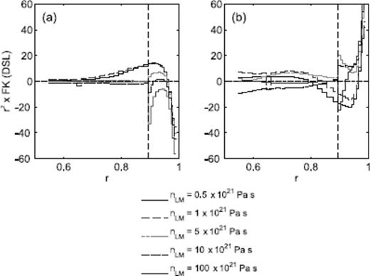
In Fig. 6, we show the results for inversions based on three different synthetic data sets. The first (solid line) represents an inversion of the 14 site pairs in the NL study for which observed values were provided. The second (dashed line) extends this data vector to 50 pairs of sites from Australia and the South Pacific (these sites are taken from the broader range of locations listed in the NL study, but for which observed data was not provided). The third inversion (dotted line) includes the same 14 site pairs as the first data set, but in this case noise has been added to the forward RSL predictions at each site in an effort to simulate real data uncertainties. The site-specific RSL error was generated using a population of random numbers with a standard deviation of 0.3 m. The abscissa on the plot represents the iteration counter, and the horizontal dotted line shows the model [LT in frame (a) and ν_um and ν_lm in frame (b)] used to compute the synthetics (i.e. the ideal solution of the inverse problem).

Figure 6.

Results for inversions based on three different sets of synthetic data, shown as a function of iteration counter, k. In each case, the starting model is defined by LT = 96 km, ν_um = 10²¹ Pa s, ν_lm = 10²² Pa s, and the synthetic model (with and without noise applied) is LT = 71 km, ν_um = 0.5 × 10²¹ Pa s, ν_lm = 5 × 10²¹ Pa s. The remaining details of the inversions are described in the text.

Open in new tabDownload slide

The results for the inversion of DSL from 14 pairs of sites (Fig. 6) show that convergence requires on the order of 10 iterations, and is thus relatively slow. This indicates that the inverse problem retains significant non-linearity, even with the logarithmic parametrization of the viscosity. Indeed, one-step inversions will yield poor results, for example, ν_lm remains relatively close to the starting model of 10²² Pa s after a single iteration. The slow convergence is clearly a function of the information content of the 14 DSL highstands, and it is thus useful to compare the inversion with the results based on the larger data set. Extending the synthetic data set to include 50 site pairs significantly decreases the number of iterations for convergence of both the LT and ν_lm estimates, but has little effect on the convergence of ν_um.

To simulate the inversion of real data, we degrade the information content within the 14 DSL highstands by including random observation errors. In this case, it is interesting to note that convergence is still achieved at roughly 10 iterations (although the estimate for LT tends to oscillate). However, the converged values for LT and ν_um do not match the synthetic. Specifically, LT is somewhat too low, and ν_um too high. The discrepancy is relatively small for the level of observational error we have applied, but it is a first indication of a correlation between errors in the estimate of these two parameters.

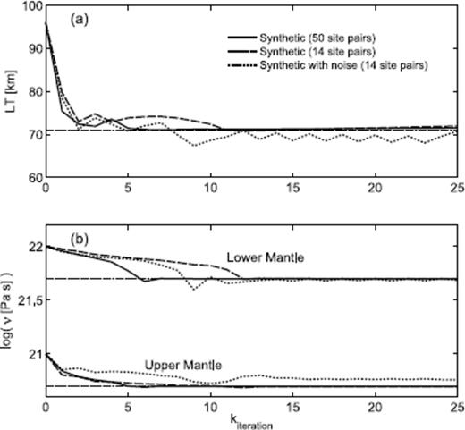
We explore this correlation further in Fig. 7, where we show the converged values of each of the three parameters as a function of the variance of the lithospheric thickness adopted in each inversion. We use the same synthetic and starting models described above, include 14 site pairs (with no errors applied) in the inversions, and a prior viscosity covariance of 50. When the prior variance for the lithospheric thickness is very small (that is, when the lithospheric thickness is constrained in the inversion to remain close to the prior value of 96 km), the viscosity in both the upper and lower mantle converge to values significantly different from those used to compute the synthetics (LT = 76 km). As we weaken the constraint on LT, and thus allow the estimate of this parameter to match more closely the synthetic model value, the viscosity estimates improve. However, these estimates do not converge to the correct values of ν_um and ν_lm until the variance of LT is set above approximately 2000 km². This exercise indicates that an accurate inference of mantle viscosity on the basis of DSL highstands requires a simultaneous estimate of (a weakly constrained) lithospheric thickness.

Figure 7.

Converged results (after 25 iterations) as a function of the covariance of the lithospheric thickness adopted in the inversion. The synthetic and starting models are described in the text. Note that the axis on the left is for the viscosity, while LT is labelled on the right.

Open in new tabDownload slide

We turn next to the case where synthetic data are inverted under the assumption that there are no a priori correlations between the individual mantle layers. That is, we no longer constrain the inversion to a two-layered viscosity model. We adopt the same starting earth model as before. Moreover, we begin with a noise-free synthetic data set consisting of DSL highstands for 14 site pairs generated from forward predictions based on an earth model defined by LT = 71 km, ν_um = 0.5 × 10²¹ Pa s and ν_lm = 5 × 10²¹ Pa s. As for the two-layered inversions, we adopt prior variances of 50 for the (log of) mantle viscosity and 3600 km² for the lithospheric thickness.

The thick solid line in Fig. 8 shows the converged model for this case. This result appears to be consistent with the model used to compute the synthetics for layers throughout the upper mantle and within the middle of the lower mantle. There is, however, disagreement at both the top and bottom of the lower mantle, where we note that the Fréchet kernels in Fig. 4 show little sensitivity. We explore this disagreement further in the next section where we present results for a formal resolving power analysis.

Figure 8.

Results of converged (after 25 iterations) inversions with no prior correlations between each of the 34 mantle layers. The thick solid and dotted lines represent inversions based on 14 and 50 synthetic DSL data, respectively. The synthetic and starting models are prescribed on the figure. In the 14 data inversion the prior variances are 50 for the (log) viscosity parameters and 3600 km² for the lithospheric thickness parameter. The former is reduced to 10 for the 50 data inversion.

Open in new tabDownload slide

3.3 Resolving power analysis

A proper comparison between the inverted model and the underlying synthetic model should be based on the resolving power of the data rather than on the results for individual model layers. To this end, we first computed the trace of the so-called resolution matrix (Backus 1988),

12

which yields an estimate of the number of independent parameters resolved by the data. For the inversion described above, the trace was computed to be ∼3. Next, we examined the posterior covariances for each target depth (as discussed in Section 2.2) to search for three radial regions that appeared to be resolved by the data (i.e. where covariances were localized about the target depth) and which yielded posterior averages that were only weakly correlated. The target depths determined in this fashion included two in the upper mantle, at 543 and 196 km depth, and one in the middle of the lower mantle, at 1692 km depth. The posterior covariances for these target depths are illustrated in Fig. 9.

Figure 9.

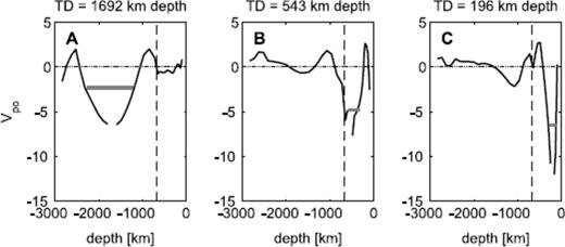
Posterior covariances for 3 different target depths (TD), as labelled on each frame, for the inversion of the 14 DSL data (thick solid line, Fig. 8). The solid grey horizontal line on each frame represents our measure of the radial resolving power at the associated target depth (see Table 2 and text). The diagonal element (i.e. the posterior variance for the given target depth) is positive and off the top-scale of the plot.

Open in new tabDownload slide

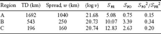
The spread of the covariances provides the first detailed measure of the radial resolving power of the NL data set, and the thick horizontal line on each frame represents the radial region over which averages were obtained. These lines define three radial regions extending from 110 to 270 km, 320 to 570 km and 1225 to 2265 km depth; that is, spreads of ∼160 to ∼250 km for the two upper mantle targets and ∼1040 km for the target in the middle of the lower mantle.

Table 2 provides the volumetric average of the inverted model values within each of these three regions (labelled as A, B and C). These averages are 20.73 and 20.74 within the upper mantle, and 21.68 in the lower mantle, in excellent agreement with the averages of the model used to compute the synthetics (20.69 and 21.69 in the upper and lower mantle, respectively). We conclude that the inversion has accurately retrieved averages of the synthetic model over the three radial regions resolved by the 14 DSL data. The inversion also yields an estimate of the lithospheric thickness of 73.7 km, which is in good agreement with the value (LT = 71 km) used to compute the synthetics.

Table 2.

Results of the inversion for each of the target depths considered in Fig. 9.

Open in new tabDownload slide

The table also shows the posterior and prior standard deviation, as well as the ratio of the variances, as defined in eq. (10), for each of the three mantle averages. These ratios indicate, as expected, that the data significantly reduce the uncertainty in model averages when these averages are taken over regions consistent with the resolving power of the data set. In contrast, the variance reduction associated with an estimate of individual model layers is far less significant. As discussed above, the three regions A—C were also constrained to yield relatively small posterior correlations. Indeed, the posterior cross-correlation coefficients, defined by

13

were computed to be ρ_ab = 0.05, ρ_ac = −0.07 and ρ_bc = −0.11. (The prior correlation coefficients were, for this inversion, zero.)

The inversion shown by the thick solid line in Fig. 8 makes clear the limited information content of the 14 DSL data. These data resolve relatively fine structure in the upper mantle, but the resolving power within the lower mantle is significantly weaker and confined to the middle of this region. As in the last section, we performed a test in which we inverted a larger data base of 50 DSL synthetics. The results for this case (thick dashed line, Fig. 8) suggest significantly improved resolution of shallow (top 500 km) lower mantle structure.

4 Conclusions

In this paper, we have revisited the influential analysis performed by Nakada & Lambeck (1989) and Lambeck & Nakada (1990) using an updated sea-level theory and a formal Bayesian inverse theory in order to examine the resolving power of their original data set.

The non-linear, iterative inversion of highstand data requires the calculation of Fréchet sensitivity kernels. We have found that although the site-specific RSL predictions showed the greatest sensitivity to viscosity variations within the upper mantle, there was a non-negligible sensitivity to variations of lower mantle viscosity. Local continental levering effects caused the former sensitivity to vary dramatically from site to site; in contrast, the latter senstivity resulted from long-wavelength ocean loading and syphoning effects and, therefore, showed a similar trend from site to site. Thus, although the DSL predictions (which consider the difference in the highstand amplitude between pairs of sites) retained a strong sensitivity to variations in the upper mantle viscosity, the sensitivity to lower mantle viscosity variations was partially cancelled. Nevertheless, we found that at many site pairs, the sensitivity of DSL predictions to a bulk variation in the lower mantle viscosity was comparable to a similar bulk variation in upper mantle viscosity. The sensitivity of the DSL predictions to changes in lithospheric thickness was also examined; site pairs that lie parallel to the broad, levering-induced tilt of the coast show less sensitivity to this parameter than do site pairs that lie perpendicular to the tilting (see NL).

The inversions were based on synthetically-generated DSL highstands, beginning with results based on a prior assumption of a two-layered viscosity model. In this case, the inversion of DSL from 14 pairs of sites showed a relatively slow convergence, indicating that, despite the logarithmic parametrization of the viscosity, the inverse problem retains significant non-linearity. The rate of convergence significantly improved when a larger set of 50 synthetic DSL data were used. Degrading the original 14 DSL highstands by including random observation errors did not significantly reduce the rate of convergence; however, the converged values of the lithospheric thickness and the upper mantle viscosity did not match the earth model used to generate the synthetics. Furthermore, an accurate inference of mantle viscosity on the basis of DSL highstand requires a simultaneous estimate of (a weakly constrained) lithospheric thickness.

Next, we performed an inversion in which no prior correlation between model parameters was included. In this case, the posterior covariance matrix indicated that the data resolved the volumetric average viscosity within three radial regions extending from 110 to 270 km, 320 to 570 km and 1225 to 2265 km depth. The posterior volumetric averages computed over these regions, as well as the lithospheric thickness, were all in excellent agreement with the model values used to compute the synthetics. Moreover, the posterior variances of these averages were reduced by a factor of 3–7 from the prior variances. This indicates that the DSL highstand data have a resolving power that is better than is captured by forward analyses based on isoviscous upper and lower mantle regions.

In future work, we will extend these estimates of resolving power to invert a set of DSL highstands compiled from the geological record. A preliminary analysis of the specific observational constraints adopted by NL at the 14 site pairs listed above was characterized by relatively unstable inversions. Accordingly, our extended analysis will incorporate newer observational constraints collected over the last two decades (e.g. Belperio et al. 2002). The synthetic inversions described above (e.g. Fig. 8) suggest that it may be possible to improve the resolution of radial viscosity structure inherent to the NL data set, particularly in the shallow lower mantle, by extending the number and coverage of the DSL site pairs. Constraints derived from an improved and expanded data set could then be compared with those derived from other load-insensitive regional data sets (site-specific decay times from Hudson Bay and Fennoscandia, and the Fennoscandian Relaxation Spectrum) to formally assess the necessity of invoking lateral variations in Earth structure.

Acknowledgments

This work was supported by GEOIDE, NSERC, and the Canadian Institute for Advanced Research.

References