


Summary
Magnetic variation (MV) surveys show a 40 km wide zone of high electrical conductivity in the middle crust extending across the Southern Uplands of Scotland from the North Sea to Galloway. A new magnetotelluric (MT) survey across the conductor in Galloway was designed to improve the resolution of structure in the depth range 1–15 km, and, at the same time, assess the improvement in resolution that could be achieved in a practical situation by optimizing data acquisition, processing, analysis and modelling. A 40 km long profile was measured, doubled for part of its length at a separation of 1 km, with a typical site spacing of 2 km or less. It was supplemented by shorter parallel and orthogonal lines, giving a total of 40 sites.
Galvanic distortion models involving regional 2-D structures gave poor fits to the impedance tensors both for the array as a whole and for individual sites, confirming the picture from induction arrow maps that many sites were influenced by 3-D structures on scales of a few kilometres and upwards. Other indicators of the electrical strike (regional and local MV measurements, the spatial structure of the Groom—Bailey regional impedance phase and of the rotated off-diagonal phase), gave values more in agreement with the geological strike of N52°E, which was adopted as the most appropriate coordinate system into which to resolve the data. The MT impedances were accordingly rotated into directions N38°W (‘TM’) and N52°E (‘TE’), and inverted using the 2-D code of Rodi & Mackie. The investigation explored the sensitivity of the outcome to a wide range of starting model resistivities and roughness parameters, and to different data subsets. The ‘TE’ mode data were insensitive to structural detail, and the best fit achieved was unacceptable, suggesting the influence of structure outside the plane of the section. The ‘TM’ mode data could be fitted satisfactorily by varying the model roughness and gave the best control on the geometry of the conductive bodies. Forward modelling showed that the model generated from the ‘TM’ mode also fitted the MV data adequately.
The inversion resolved the conductive zone into distinct blocks, with edges matching faults mapped in the surface geology: the Leadhills, Fardingmullach and Orlock Bridge Faults, and the Moffat Valley lineament. In the resistivity image, the faults are vertical structures, disrupting other features to a depth of 15 km, which agrees with the view that, although they originated as thrusts, they were reactivated by strike-slip motion during oblique closure of the Iapetus Ocean. Within some of the blocks are highly conductive regions, no more than 4 km wide. The most likely explanation is graphite or other metallic mineralization, localized in shear zones.
1 Introduction
The electrical conductivity of the crust beneath the Southern Uplands of Scotland has been investigated by repeated electromagnetic surveys, from Edwards (1971) to Banks (1996) (see the latter paper and Livelybrooks 1993, for a list of references). Magnetic variation (MV) surveys at periods between 200 and 2000 s provide a regional-scale picture of conductive structures in the upper and middle crust. Fig. 1 is a hypothetical event map of the anomalous horizontal magnetic field at a period of 750 s. It has been computed from single-station transfer functions using the procedure described by Banks (1993), but incorporating measurements from two new surveys, one by Junge (1995) extending coverage in the north and northeast, and one in the southwest, described in this paper. The parameters of the hypothetical event analysis have been chosen to optimize the spatial image of the conductor that runs northeast to southwest across the Southern Uplands, though they also provide a less optimal view of the conductor that runs east to west across northern England.
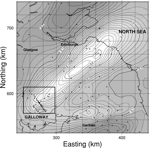
Magnetic variation anomalies in northern Britain. The map is a simulation of the horizontal magnetic field in the direction N45°W associated with a 1 nT horizontal magnetic field, direction N135°E at a reference site (Eskdalemuir magnetic observatory). The period of the electromagnetic field is 750 s. The direction of the horizontal field has been chosen to produce an undistorted image of the scattered currents created by a conductor aligned at N45°E. The anomaly maxima lie directly above the currents. Dots mark the positions of observations. The dense array of points surrounded by a box is the survey described in this paper. The box corresponds exactly to the area displayed in detail in Fig. 2.
The new surveys confirm the continuity and horizontal extent of the conductor (at least 150 km), and precisely constrain its position in relation to the surface geology. It closely follows the trends of the major Caledonian faults and structural boundaries in the Southern Uplands (such as the Southern Uplands and Orlock Bridge Faults), changing orientation with them from N35°E in the northeast to N45°E in the southwest. The vertical magnetic field at the surface can be continued down to an equivalent current system in a thin sheet at a depth of 10 km (Banks 1979). The zone of enhanced currents, approximately 40 km wide, stretches from just southeast of the Southern Uplands Fault to 5 km southeast of the Orlock Bridge Fault, involving several of the crustal units into which the Southern Uplands is divided (see Fig. 2). Banks (1996) suggested that the high conductivity was caused by graphite distributed throughout a block of meta-sedimentary rock that had been trapped at mid-crustal levels during the closure of the Iapetus Ocean. However, the high conductivity might instead be confined to a thin sheet marking the detachment zone where the Southern Uplands accretionary complex was thrust over the Avalonian basement rocks. The movement could have assisted conversion of the carbon-rich Moffat Shales to graphite (Jödicke 1992; ELEKTB group 1997).
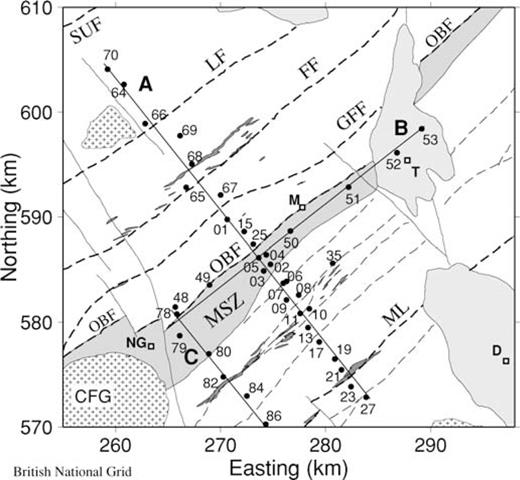
Location of MT sites (filled circles) in relation to Galloway geology (see Fig. 1 for the location of the map area). Black dashed lines, NE—SW tract-bounding faults (Caledonian); continuous lines, NW—SE normal faults (Carboniferous); unshaded areas, Ordovician and Silurian greywackes; light-shaded areas, Carboniferous/Permo-Triassic sediments; thin dark streaks, carbonaceous shales; broad dark zone (MSZ), Moniaive shear zone; ++, granite batholiths (CFG, Cairnsmore of Fleet). SUF, Southern Uplands Fault; LF, Leadhills Fault; FF, Fardingmullach Fault; GFF, Glen Foumart Fault; OBF, Orlock Bridge Fault; ML, Moffat Line. D, Dumfries; T, Thornhill; M, Moniaive; NG, New Galloway.
Magnetic variation measurements are a valuable tool for mapping the lateral extent of conductors but provide only limited constraints on their depth. Magnetotelluric (MT) measurements are much more effective in this respect. Banks (1996) compiled a database of the existing MT surveys of the Southern Uplands (referenced in Livelybrooks 1993), and added new sites to create a composite profile that crossed both of the conductive structures shown in Fig. 1. Most of the new measurements were concentrated in the southern section, and the improved data quality led to a much more detailed image of the southern conductor. Because of the wider station separation and poorer quality TM mode data, the northern conductor was less well resolved. It appeared as a single feature in the electromagnetic image, continuous across strike, and of uncertain depth extent, and the 1996 survey was unable to determine its relationship to structures seen at the surface. A new survey was required, designed to resolve structure at depths between 1 and 15 km. It also provided the opportunity to assess the improvement in resolution that could be achieved in a practical situation by optimizing as many as possible of the different phases of MT data acquisition, processing, analysis and modelling.
2 The Survey Area and its Geology
2.1 Choice of survey area
The area selected was in Galloway, in southwest Scotland. Previous MV surveys suggested that the conductive structure continues southwestwards from the profile investigated by Banks (1996). A short MT line in the Thornhill basin (Beamish 1995) indicated that the crust below 8 km was moderately conductive. It also detected narrow conductive zones in the upper crust, possibly associated with the Caledonian faults. Galloway is largely rural, so that low levels of cultural noise could be anticipated. The area has been the target of detailed geological remapping by the British Geological Survey (Barnes 1995; Phillips 1995), and structures there are probably better known than in any other part of the Southern Uplands. With a single 40 km profile (see profile A in Fig. 2), it was possible to traverse a number of features, each of which (if associated with a mineral such as graphite) were potential conductors. They were: outcropping carbonaceous (black) shales repeating near the base of each thrust-bounded block of crust; a thrust that had been reactivated as a strike-slip fault during the closure of the Iapetus Ocean (the Orlock Bridge Fault); and a ductile shear zone (the Moniaive Shear Zone) which accommodated the strike-slip motion at a deeper level. A high-resolution MT survey might establish whether there were a physical connection between one or more of these structures and the region of high conductivity known to be present at depth. The existence of such a link would place important constraints on explanations for the high conductivity.
2.2 The geology of the survey area
It is thought that the Southern Uplands formed in Ordovician and Silurian times as an accretionary prism on the Laurentian margin of the Iapetus Ocean. Wedges of sediment were thrust over one another, creating a series of tracts bounded by thrust faults. Within each tract, the sediments were young to the northwest, but overall the tracts become progressively younger in a southeasterly direction. The sediments are predominantly greywackes, but carbonaceous shales (the Moffat shales) are present towards the base of each tract (Fig. 2). During the closure of the Iapetus Ocean, the entire accretionary wedge was thrust to the southeast over Avalonian basement. The detachment surface over which movement occurred is thought to be at a depth of 8–10 km (Leggett 1983). The weakness of the shales may have assisted the movement. As the Iapetus ocean closed, Avalonia moved obliquely relative to Laurentia. Some of the NE—SW-aligned structures, such as the Orlock Bridge Fault, are believed to have been reactivated as sinistral strike-slip faults to accommodate the motion (Phillips 1995). For over 100 km, the southern margin of the Orlock Bridge fault is formed by a ductile shear zone up to 5 km wide—the Moniaive Shear Zone. This zone probably represents a deeper and earlier expression of the sinistral deformation associated with the closure of Iapetus. During the Carboniferous period, vertical movement occurred along NW—SE faults. Consequently, the structural level exposed by erosion changes along strike, with the deepest levels exposed in the area between the Cairnsmore of Fleet granite and Moniaive (Stone 1995). Although the main lithological and structural boundaries are aligned NE—SW, any associated conductive features may have been disrupted by the later faulting, creating 3-D structures.
3 Field Measurements
3.1 General considerations in the design of the survey
An important element in the experimental design was the need to achieve a small station separation on the main MT profile (A in Fig. 2). Although the lithology of the surface rocks is relatively uniform, they are cut by faults, shear zones and black shales, and our aim was to try to detect and trace conductive zones associated with these narrow features as close to the surface as possible, so that they could be identified. Any spatial redundancy in the measured impedance would also help in the detection and correction of static shifts. In practice, a spacing of 1–2 km proved to be a reasonable compromise between what was logistically feasible and what was desirable for optimum resolution. The effect of small-scale heterogeneities and larger-scale 3-D structures outside the line of the main profile is often assessed by decomposing the impedance tensor at each site under the constraint of a limited 3-D model (Bahr 1988; Groom & Bailey 1989). We felt it was essential to support the results from such analysis by a limited form of 3-D survey. The SPAM III data acquisition system (Ritter 1998), has the facility for recording data from a local base simultaneously with one or more remote sites, linked by up to a kilometre of digital cable. We made use of the capability to establish two parallel profiles on the main line, separated by the 800 m length of digital cable. By comparing the results, the consistency of the structure along strike could be assessed. Unfortunately, the transputer-based network proved to be vulnerable to interference from animals, etc., which caused the system and the recording to hang up. As a result, only part of the profile was duplicated. However, the main line was also supplemented by a shorter parallel profile a few kilometres away (C in Fig. 2), and by a number of separate sites forming a widely spaced profile parallel to the geological strike (B in Fig. 2). Recordings from independent systems were synchronized for remote reference processing by GPS timing.
3.2 Data acquisition
The main MT profile (profile A in Fig. 2) was aligned perpendicular to the strike of the principal Caledonian structures (N55°E). Its location was largely determined by access and communications. Two experiments were carried out, in 1997 October and 1998 October, each of 4 weeks duration. The first utilized a total of seven SPAM III data acquisition systems, two from the Natural Environment Research Council (NERC) Geophysical Equipment Pool, two from Edinburgh, two from the GeoForschungsZentrum (GFZ), Potsdam, and one from the University of Frankfurt. The bulk of the induction coils (Metronix MFS05) and silver/silver chloride electrodes were supplied by Potsdam; the NERC pool contributed CM11E coils. With this equipment, we were able to keep as many as six MT sites operational at any time, including one running continuously at a fixed location. The equipment at each site was programmed to the same pattern of data acquisition, synchronized by GPS. SPAM III is capable of continuous sampling at a rate of 512 Hz for all frequencies less than 128 Hz. However, to reduce the volume of stored high-frequency data, the two highest-frequency bands were recorded in a scheduled mode of hourly samples lasting 2 min (128–16 Hz) and 17 min (16–2 Hz). Frequencies less than 2 Hz were sampled continuously. At least two runs of 2.5 d were recorded at each site. The very highest-frequency band (1000–100 Hz) was acquired with daytime runs of a few hours duration.
The second experiment was on a smaller scale, aimed at filling in gaps left by the first and adding longer-period measurements at key locations. Unfortunately, problems with the prototype of the NERC long-period logging system prevented the acquisition of any long-period MT data. However, the bandwidth of the Metronix coils was such that the data they generated covered most of the frequency range required to penetrate the conductive middle crust. A further nine SPAM III sites were occupied.
One possible contribution to noise in the impedance data, relative to a 2-D interpretative model, is static shift caused by small-scale lateral variations in the resistivity of the surface layer. We intended to make use of the capability of the SPAM III system for multichannel input to detect and correct for local distortions in the electric field. At a number of sites electric field data were acquired with a range of different dipole lengths and geometries. These experiments showed that static shift effects were present on a scale of tens to hundreds of metres, and were related to topography of the bedrock surface beneath the cover of wet, peaty soil. However, the logistics of laying out complex networks of cable in forested areas proved difficult. Improving noise rejection using arrays of electrodes may only be feasible in much more open country. We relied instead on the close site spacing and the doubling of the profile to detect and correct for static shift effects. As it turned out, 3-D structures on a scale of kilometres rather than tens or hundreds of metres proved to be a more severe problem.
4 Response Estimation
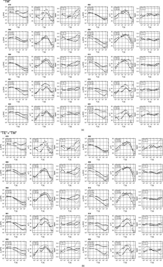
In all, 50 Gbytes of data were acquired at 40 sites, much of it of very high quality thanks to the low cultural noise levels. For most sites, robust remote reference processing (Egbert & Booker 1986) generated consistent, high-precision estimates of the MT impedance and MV transfer functions. The consistency of the resistivity and phase data was tested using the ρ+ approach of Parker & Booker (1996), which also helped to identify suspect estimates in the dead band, and to establish an error floor of 3 per cent for the impedance values. Fig. 3 shows the impedances expressed in geographical coordinates (X, north; Y, east) at four representative sites distributed along the main profile. The dashed lines on each diagram show the ρ+ response that best fits both the apparent resistivity and phase, together with the 68 per cent confidence limits on it. Values plotted as open circles were judged to be incompatible with the ρ+ response, and were rejected. They are commonly in the period range from 0.1 to 10 s, which includes the ‘dead band’. A different problem was identified at the most southerly locations on the profile, of which site 19 is representative. The data quality is good, but the phase of the impedance, φYX, exceeds 90° at periods beyond 100 s, suggesting strong 3-D effects. At site 10, the high phases across much of the measured frequency range signal the presence of a very strong conductivity anomaly.
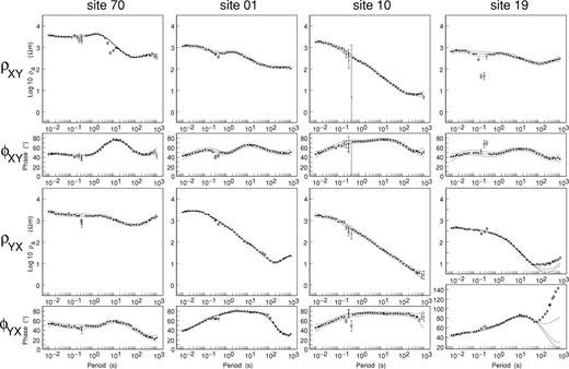
Apparent resistivity (ρXY and ρYX) and phase (φXY and φYX) responses measured in geographic coordinates (X, north; Y, east) at representative sites 70, 1, 10 and 19 on profile A (Fig. 2). The dashed lines show the best-fitting ρ+ response and the 68 per cent confidence limits. The outliers in the dead band, marked by open circles, are subsequently excluded on the basis of the ρ+ analysis.
5 Strike Determination
5.1 Induction arrow maps
A key step is to decide whether the data are compatible with a 2-D conductivity model, and to identify the electrical strike direction. One approach is to use the magnetic variation response. At periods greater than 100 s, the MV transfer functions for the Galloway sites are broadly consistent with the regional picture. The induction arrows (Fig. 4) indicate the presence of a 2-D conductor, aligned N45°E and concentrated beneath and to the south of the Orlock Bridge Fault. Even at 114 s, however, the real arrows at sites south of the Moniaive Shear Zone suggest the additional influence of a conductive structure to the east of the main profile. The arrows are tiny, but very consistent both in their magnitude and direction. The influence of the second conductor grows as the period decreases. The spatial pattern of arrows at 5 s period (and, less clearly, at 0.5 s) is suggestive of a conductive block running NE—SW and coinciding with one of the belts of black shale, but terminating east of profile A. The structure might be created by changes along-strike in the depth or thickness of the principal conductor. Vertical displacements on the NW—SE Carboniferous faults could cause such changes. Faults are marked immediately to the east of profile A, and also further east, associated with the Thornhill Basin. In the absence of more sites in the east of the area, we cannot say which is more likely to be responsible. What is clear from the MV data is that the overall 2-D regional structure (strike ∼N50°E) is disrupted by 3-D features with a spatial scale of a few kilometres, which most strongly influence the fields at periods less than 5 s.
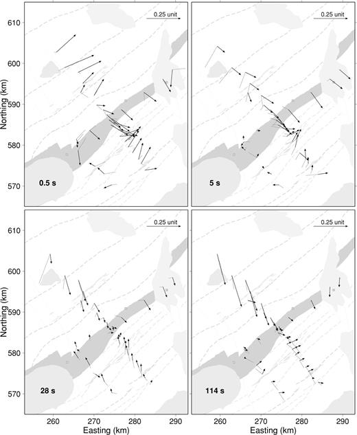
Maps showing the spatial variability of the induction arrows (Parkinson convention) at representative periods. Solid arrows are the real vectors; dotted lines the imaginary. The arrows are superimposed on a map of the main geological structures displayed in Fig. 2.
5.2 Hypothetical event analysis of the MV response
When the size of 3-D inhomogeneities is small relative to the scalelength of the electromagnetic field, the scattered electric field is in-phase with the regional field. If the regional structure is 2-D, the impedance tensor and MV response simplify when the response is predicted for fields aligned with the regional strike. Ritter & Banks (1998) suggested using Argand diagrams of the vertical magnetic field generated by hypothetical event analysis, to detect the event direction that gave a consistent phase at sites in an array. Fig. 5 shows Argand diagrams of the Galloway response at a period of 750 s for a range of hypothetical event directions. The most consistent phase is generated when the horizontal field direction is N140°E, indicating a strike of N50°E. This is typical of the results for the period range for which the scattering model appears to be appropriate. At periods of less than a few tens of seconds the response is controlled by local induction effects.

Hypothetical event analysis (Ritter & Banks 1998) of the Galloway MV data for a period of 750 s. θ is the direction (degrees E of N) of the hypothetical event in the horizontal magnetic field. The phase of the vertical magnetic field has a consistent value at all sites when θ lies between 120° and 150°. Further refinement suggests that the optimum value of θ is 140°, indicating a strike direction of N50°E.
5.3 Single-site Groom—Bailey analysis
Conventional (single-site and frequency-by-frequency) Groom—Bailey decomposition (Groom & Bailey 1989) and similar multifrequency, multisite analysis (McNeice & Jones 2001) also relies on a model in which the regional structure is assumed to be 2-D, with the local electric field at each site influenced by galvanic distortion. Application of the method generates correct values for the regional strike as long as the model itself is correct, but gives misleading answers when the actual structure is 3-D (Simpson 2000). Fig. 6 shows the Groom—Bailey parameters at site 1. The regional strike has a consistent orientation between 0° and −15° over three decades of period, but becomes unstable at periods shorter than a few seconds. Also, the fit of the model to the measured impedance is poor over most of the observed range of periods, and the same is true for many of the sites.
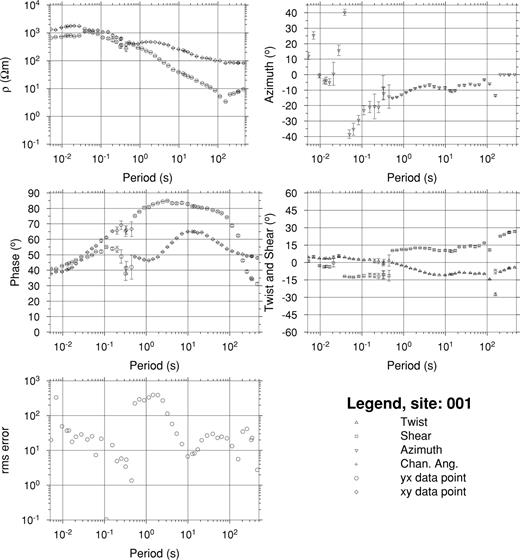
Groom—Bailey single-site parameters for site 1. A strike angle (azimuth) between 0° and −15° is indicated, but the fit of the model is poor.
5.4 Multisite Groom—Bailey analysis
If an array of sites is influenced by the same 2-D regional structure, the measured impedances can be rotated to the same selected direction, the galvanic distortion model fitted to each, and the misfit summed over all the sites. The rotation angle is then varied to find the direction that gives the best overall fit to the observations (Smith 1995). Fig. 7 shows how the misfit varies with rotation angle for five periods that span the range investigated. At none of the periods (with the exception of the longest) does the model fit the data well. The difference at 750 s is that the error bounds on all the impedances are substantially wider. At most periods, the misfit is relatively insensitive to the rotation angle. However, the angle that minimizes the misfit does change systematically with period. At 0.05 s it is N55°E, in agreement with the geological strike. At 0.5 s, it has rotated to N70°E, at 5 s it is N85°E and at 50 s it is due east. At the longest period it rotates back to N80°E. Such behaviour could be interpreted as being the result of a change of electrical strike with effective depth of penetration. However, because of the poor performance of the model in describing the observations, and the likely importance of intersite variability, it would be unwise to give much weight to this result.
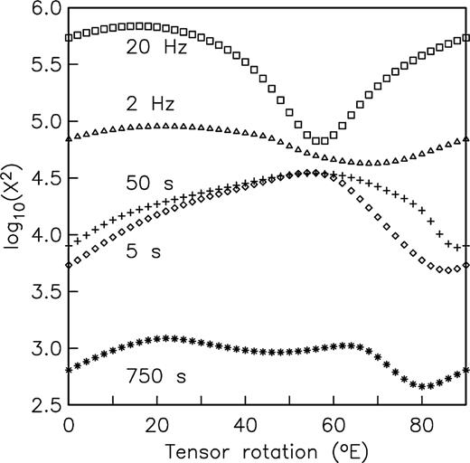
Dependence of misfit (summed over all sites) on the angle through which the impedance tensors at all sites are rotated. The model fitted is a 2-D regional structure with local galvanic distortion (Smith 1995). Except at 20 Hz, the misfit is relatively insensitive to the rotation angle. The suggested strike angles vary from N55°E to N90°E.
5.5 Maps of the Groom—Bailey regional phases
Given the indications that the underlying assumption of the Groom—Bailey approach (that the regional structure is 2-D) is inappropriate, we decided to seek a method of quantifying the directionality of the electromagnetic field data that was not model-dependent. The information that is not used in the Groom—Bailey decomposition is the spatial organization of the measurement sites, and the spatial structure of the fields. One of the problems in quantifying the spatial structure is the impact of static shift and galvanic distortion in causing intersite variability on a scale smaller than the site separation. As a way of minimizing the aliasing of the structure, we took as our measure of the electromagnetic field the values of the regional TE and TM mode impedance phases extracted at each site using the Groom—Bailey approach. These parameters should possess spatial consistency not to be expected from the raw impedances because of the local distortion. Fig. 8 shows maps of the single-site Groom—Bailey rotation angle and TM and TE mode phases at three representative periods. Although the number and distribution of sites is limited, the spatial structure of the TM mode phase is reasonably well constrained by the two NW—SE profiles, and shows that, for periods between 3 and 300 s, the strike angle is around N45°E, and consistent with the geology.
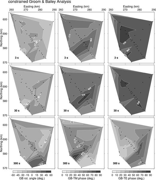
A comparison between the optimum Groom—Bailey angle and the spatial structure of the TM and TE mode phases. The preferred Groom—Bailey rotation angle is small (<15°) everywhere except in the extreme southeast. In contrast, the phases (particularly the TM mode) of the ‘regional’ impedance, independently determined at each site, follow the geological strike.
5.6 Power spectra of phase maps
The use of the Groom—Bailey parameters is clearly unsatisfactory as a complete solution to the problem of quantifying the spatial structure of the field, because it still incorporates the assumption that the regional structure is 2-D. To avoid this element entirely, we have used the phase of the Zxy element of the impedance tensor at a given period, rotated at all sites to the same selected azimuth. The geometry of the phase map can be characterized by the spatial covariance function or its Fourier transform, the 2-D spatial power spectrum. The power spectrum is most readily determined by computing the Fourier transform of the data, but this requires it to be interpolated on to a regular grid. Given the limited spatial coverage of our network, we can expect considerable uncertainty in the resultant spectrum. The algorithm we have used to grid the data is one that uses all the measured data, weighted according to the distance of the sites from the required grid points. It deals relatively well with the problem of simulating data outside the measurement area, and also in avoiding short-wavelength features associated with closely spaced sites.
2-D features in the map appear as high-power structures along radial lines in the power spectrum, oriented at 90° to the anomalies. In order to quantify the directionality of the phase anomalies, we sum the power in pie slices in the wavenumber domain, each defining an equal angular range δφ (φ= tan −1ky/kx, where kx and ky are the components of the wave vector in the x and y directions, respectively). A plot of the power against φ quantifies the relative importance and 2-D of anomalies with different directions. To investigate the change in the map as the excitation (direction of the horizontal magnetic field) is varied, we recompute P(φ) as the rotation angle (θ) of the impedance tensor is varied between 0° and 180°, and plot the power as a function of φ and θ. Fig. 9 shows the outcome for a period of 50 s. ‘2-D’ structures should respond to excitation by a range of horizontal field directions, with maxima at 90° to the strike of the structure (the TE mode) and parallel to the structure (the TM mode). These maxima are likely to be different because of the difference in response of the structure to the two modes—the TE phase anomaly is distributed over the width of the conductor, while the TM phase anomalies are associated with the boundaries (see, e.g., Weidelt 1975). The maximum power at any excitation should correspond to the alignment of the structure. Two such features appear in Fig. 9, indicating structures aligned N5°W and N25°E. The latter feature changes with period and clearly relates to structures in the corresponding maps. The former is a fairly consistent feature at all periods, and may be an artefact generated by the site distribution and gridding procedure. Its presence suggests that we should be very cautious in drawing any firm conclusions concerning the strike using this method when the site distribution is restricted. However, we feel that the approach has many merits for analysing electromagnetic fields associated with complex 3-D structures, and will show its value in situations where the site distribution is more regular.
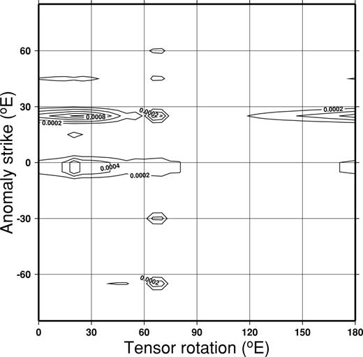
Distribution of power with azimuth in response to different rotation angles of the impedance tensor. The y-axis is the strike direction of 2-D features in maps of the phase of the Zxy component of the impedance tensors. The tensors at all sites are rotated through the angle specified on the x-axis. This angle can be thought of as the direction of the regional electric field created in response to a uniform horizontal magnetic excitation at 90° to it. The period of the electromagnetic field is 50 s.
5.7 Interpredictability of TM mode apparent resistivities and phases
One further way of deciding whether the correct strike angle has been selected is to test the compatibility of the rotated TM mode apparent resistivities and phases (Parker & Booker 1996). For a 2-D structure, the TM mode phases should be predictable from apparent resistivities and vice versa, which suggests that the interpredictability could be used to test whether the chosen strike direction (and implied TM mode direction) is correct. The procedure adopted was to rotate the impedance tensor to a specified angle, and attempt to fit a D+ model to the combined apparent resistivity and phase data. The misfit of the model is plotted as a function of the rotation angle. When the impedance tensors at the southern sites (already identified as showing unacceptable phases at the longest periods) are rotated in the quadrant from N45°W to N45°E, the misfit of the assumed TM mode does not show a strong dependence on the rotation angle. The misfit is marginally unacceptable for rotation angles in the range −20° to +20°, but otherwise acceptable. We decided to follow the suggestion of Parker & Booker (1996), and also test the assumed TE mode. The misfit of the D+ model to the combined data set (bottom panel in Fig. 10) strongly discriminates against rotation angles between −20° and +20°, and the best fit is achieved for an angle between N35°W and N45°W. When the impedance tensor is rotated to N38°W, the TE phase lies in the correct quadrant and the apparent resistivity and phase are mutually compatible. On its own, this cannot be regarded as a ‘strong’ result, since it is not known under what conditions the TE response should pass the 1-D response test. However, the difference in sensitivity of the phase response of the two modes to 3-D effects is itself an indicator that they have been correctly identified. These pieces of evidence should be regarded as a small reinforcement of all the others assembled in support of the selected strike direction.
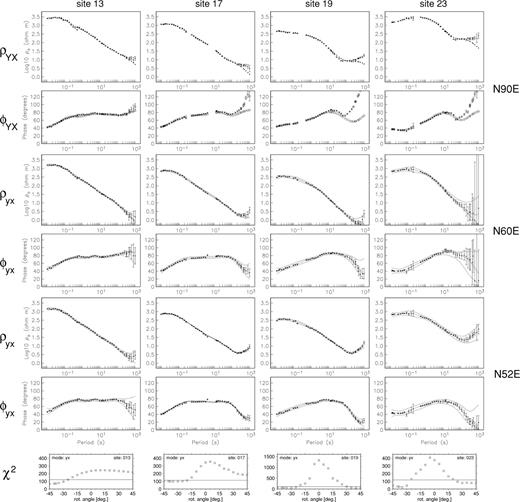
Apparent resistivity (ρyx) and phase (φyx) responses for sites on the main profile south of the Orlock Bridge fault. The impedance tensors have been rotated into directions that correspond to electric field alignments of N90°E, N60°E and N52°E. The lowest graphs display the χ2 misfit of the ρ+ analysis for individual sites as a function of the angle (relative to geographic north) through which the impedance has been rotated. The horizontal line marks the limiting value for an acceptable misfit.
5.8 The choice of reference directions
It is unfortunate that analysis of the impedance tensor fails to give a clear answer to the question of whether a 2-D model is adequate, and if so which directions best represent the TE and TM modes. The tensor decomposition model fails to fit the observations adequately, either when the entire array is considered, or at the level of a single site. The electromagnetic environment of the majority of the sites must be influenced by electrical structures that are 3-D on a scale, which is significant when compared with the inductive scalelength, rather than being much smaller as the galvanic distortion model assumes. The cause of the 3-D effects may be structures on a scale of kilometres or more, such as the changes along strike caused by the later cross-cutting faulting. Alternatively, they could be rock fabrics representing the response to changing patterns of deformation with depth, which could be treated numerically as a form of anisotropy (Heise & Pous 2001).
In this situation, we are driven back to those observations that directly relate to the spatial structure of the electromagnetic fields and the conductivity. The regional MV observations (Fig. 1) give the clearest image of the fields. That they also correctly identify the regional alignment of the conductive structures is shown by the models that have been derived from MT surveys that cross the MV anomaly at widely separated points along its length: at (347E, 666N) in East Lothian (Sule & Hutton 1986; Sule 1993), at (314E, 634N) (Banks 1996) and at (290E, 600N) (Beamish 1995). The agreement between the implied conductivity alignment, the geological structures and the orientation of other geophysical anomalies, particularly gravity, has convinced us that the directions to which we should rotate our electromagnetic observations in order to achieve the greatest simplicity are N38°W and N52°E. Because of the importance of the 3-D effects, these directions cannot be regarded as representing the TM and TE modes in the conventional sense. It is, however, convenient to label them as ‘TM’ and ‘TE’. Because the decomposition model is invalid, we have not used it to extract ‘regional’ impedance values from the measured tensors, but have simply rotated them to our preferred directions. Note that, because the main profile was aligned on the basis of the geological strike, its direction coincides with that of the ‘TM’ axis.
6 Mt Pseudo-Sections
Fig. 11 shows pseudo-sections of the ‘TM’ and ‘TE’ mode phases along the main profile (A in Fig. 2). Because of the 3-D effects discussed in Section 5, structures outside the line of the profile may contribute to some features in the pseudo-sections. In both the ‘TE’ and ‘TM’ mode sections the upper and middle crust can be loosely divided into three ‘layers’. The resistivity of the surface layer is high (greater than 1000 Ω m) and uniform. It clearly corresponds to the Ordovician and Silurian meta-sedimentary rocks. At frequencies less than 10 Hz, the phase of both modes increases to values in the range 60°–70°, indicating the presence of an underlying conducting layer. Only at periods beyond 100 s does the phase fall again, showing that the deepest layer penetrated is resistive.
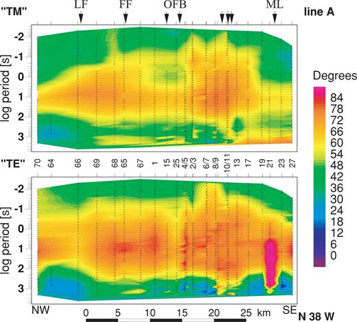
Pseudo-sections of the ‘TM’ and ‘TE’ mode phases along profile A in Fig. 2. The data were rotated into a direction N52°E. The ‘TM’ component is parallel to the profile, the ‘TE’ component along strike. The crosses show the coverage of the impedance estimates in space and frequency. LF, Leadhills Fault; FF, Fardingmullach Fault; OBF, Orlock Bridge Fault; ML, Moffat valley lineament.
The ‘TE’ and ‘TM’ mode phases are noticeably different in their resolution of structure. The lateral variations in the ‘TE’ mode phase are generally smooth, with the exception of the high-frequency, high-phase feature immediately south of the Orlock Bridge fault (sites 6–9). Previous surveys of the Southern Uplands conductor (Livelybrooks 1993; Banks 1996) relied heavily on the TE mode data because its quality was higher than that of the TM mode. Features such as this were interpreted by models in which the conductive layer shallowed from 8 to 3 km depth. However, the ‘TM’ mode pseudo-section is able to resolve more complex structure across strike. It shows there are two principal conductive blocks separated by a more resistive unit. The high density of sites and the high quality of data give us confidence that the lateral changes in phase are really as abrupt as they appear. At least three of them match closely with the location of tract-bounding faults. Proceeding south along the profile, the southward conductive—resistive transition between sites 67 and 1 coincides with the Glen Foumart fault; the strongly marked resistive—conductive transition at sites 4 and 5 is immediately south of the Orlock Bridge fault, while the conductive—resistive change at site 17 marks the Moffat Valley lineament. Whatever is responsible for the conductive layer, its spatial geometry has been modified by movements on the tract-bounding faults. Perhaps this happened when they were first created as thrusts. More probably, it occurred later when they were reactivated as strike-slip or normal faults.
The highest-frequency parts of the phase pseudo-sections are relatively featureless, with only hints of the narrow structures we hoped to detect. Where such features are derived from observations at a single site they must be interpreted with caution. The high ‘TM’ mode phase at site 68 may be caused either by the nearby outcrop of black shale, or by a 3-D structure outside the line of the section. High ‘TE’ mode phases at sites 6–9 occur just to the north of another belt of black shale outcrops, but there is nothing to be seen at sites 21 and 23, which are similarly situated. If there is a relationship between the high conductivity and the occurrence of the black shales, it is not a simple one that can be readily detected in the near-surface environment.
7 2-D Inversion
The MV data (Fig. 4) show that the electromagnetic fields at sites along profile A are influenced by 3-D fields outside the plane of the section, particularly at periods of 5 s and less. Ultimately, it will be necessary to assess the impact of the 3-D structures on the profile data by full 3-D modelling. However, 2-D modelling/inversion of the main profile is an essential first step towards constructing a model of the conductivity structure. Indeed, we hope that the first-order conductivity structures are 2-D. In order to extract them successfully, it is necessary to down-weight those features in the data that are most susceptible to the influence of the second-order 3-D structures. For instance, the effects of static shift can be minimized in initial inversions by giving greatest weight to the phase data. Its impact on the apparent resistivity pseudo-sections can be assessed and corrected for at a later stage. Larger-scale 3-D structures will affect the ‘TE’ mode data more than the ‘TM’, so initial model searches may be restricted to the latter.
‘TM’ and ‘TE’ mode response data for profile A were inverted using the 2-D code of Rodi & Mackie (2001). The starting model is a half-space of resistivity ρh. The aim of the inversion is to find the model that minimizes a penalty function made up from a combination of misfit to the observations and a measure of the model roughness, in proportions determined by a parameter τ. When τ is small, the emphasis is on achieving a good fit, which requires a rough structure. When τ is large, the emphasis is on finding a smooth model, which will necessarily fit the data less well. Considerable efforts were made to explore a wide range of the parameters and options (listed below in italics) which might influence the inversion. Their effects were judged by examining: (1) the overall data misfit of a given model as a function of its roughness (Fig. 12), and as a function of both τ and ρh (Fig. 14); (2) the distribution of rms site misfits with position along the profile (Fig. 13); and (3) the models themselves (Fig. 15).
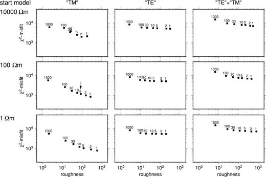
Interdependence of the data misfit (χ2) and model roughness of 2-D models obtained by inverting the combined data set (right-hand column), ‘TE’ mode alone (centre column), and ‘TM’ mode alone (left-hand column). Each plotted point is labelled by the value of τ, which determines the weight of the model roughness relative to data misfit in the penalty function minimized. Each row corresponds to a different choice of the resistivity of the half-space that is the starting point of the inversion. The arrow points to the combination of τ and ρh selected for the model displayed in Fig. 16.
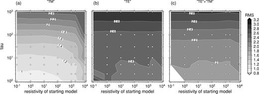
Dependence of the overall rms data misfits on the roughness weighting parameter τ and the resistivity ρh of the initial half-space. (a) Fitting the ‘TM’ mode alone; (b) fitting the ‘TE’ mode alone; (c) joint inversion of both modes.
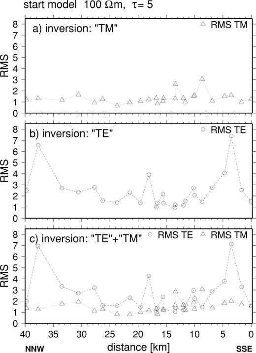
rms data misfits along profile A, fitting (a) the ‘TM’ mode alone, (b) the ‘TE’ mode alone, (c) both modes.
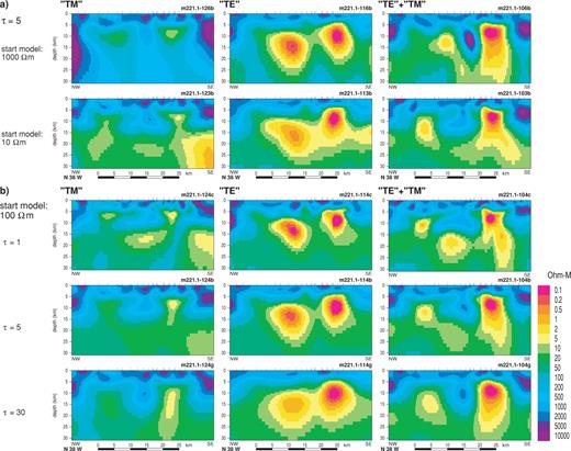
Resistivity models fitting the ‘TM’ mode (left-hand column) and ‘TE’ (centre column) modes alone, and both modes together (right-hand column). (a) Each row corresponds to a different choice of the resistivity of the half-space that is the starting point of the inversion. τ is set to 5. (b) Each row corresponds to a different value of τ. The starting point of the inversion is a half-space with a resistivity of 100 Ω m.
The structure and size of the grid delimiting the resistivity model. The size of the grid elements, particularly in the upper layers of the model, was refined until no further improvement in the misfit was achieved with all other parameters fixed.
Procedures for dealing with static shift. The likely influence of static shift was handled by down-weighting the phase data relative to the apparent resistivity in the inversion. This was achieved by assigning an error floor of 1.72° to the phase (corresponding to a 3 per cent error in the impedance), and a higher error floor to the apparent resistivity. Inversions with error floors of 6 per cent (no static shift) and 25 per cent were compared. The models generated from the ‘TM’ mode data were relatively insensitive to the choice, but it made a substantial difference to those generated from the ‘TE’ mode. The 25 per cent error floor was adopted for the remaining experiments and the final inversions.
The subset of the data that were inverted—‘TE’, ‘TM’ or both.Fig. 12 shows how the overall model misfit changes in response to the parameter τ for a range of starting model resistivities. The three columns display the behaviour when the two modes are inverted separately and together. When the ‘TM’ mode data are inverted on their own (left-hand column), the misfit decreases steadily and consistently as τ decreases and the roughness measure increases. The rougher models (τ≤ 10) generate misfits that are distributed relatively uniformly among sites along the profile (Fig. 13a), with an rms misfit of 1 sd (standard deviation). When the ‘TE’ mode data are inverted on their own, however, there is much less improvement in fit either overall or at individual sites as τ is reduced (cf.Fig. 12). The rms misfit in the centre of the profile can be as low as 1 sd, but towards the northern and southern ends generally exceeds 2 sd (Fig. 13b). Irrespective of the choice of other parameters, no model can be found that fits the ‘TE’ mode data in a wholly acceptable way. Either the errors in the ‘TE’ response observations are systematically underestimated (which seems unlikely because of the similarity in level of misfit of the ‘TE’ and ‘TM’ modes in the ρ+ analysis), or there is an inherent misfit in the ‘TE’ mode owing to the influence of structures outside the plane of the section. Whatever the cause, the choice of parameters and the resultant model should be more strongly influenced by the need to fit the ‘TM’ mode data rather than the ‘TE’ mode. As might be expected, when the combined ‘TE’ and ‘TM’ mode data set is inverted, it is the inability to find any model that fits the ‘TE’ mode that controls the response to changes in the roughness parameter and starting resistivity.
The parametersτ(which control the relative weights of data misfit and model roughness) andρh (the resistivity of the half-space that is the starting point of the inversion). Fig. 14 shows how the overall rms misfit changes in response to reducing τ (increasing roughness) from 1000 to 1, and to varying ρh between 10−1 and 104Ω m. Improvements in the ‘TM’ mode fit as τ is reduced (Fig. 14a) are achieved for a wide range of starting models (0.1 ≤ρh≤ 1000 Ω m), indicating that the data definitely require the rougher structures corresponding to 1 ≤τ≤ 5. Acceptable misfits are generated when the resistivity of the initial half-space model is 100 Ω m or less. The behaviour of the ‘TE’ mode (Fig. 14b) is very different. Reducing τ does not significantly reduce the ‘TE’ mode misfit, irrespective of the starting model resistivity. However, the models that are generated by the inversion of the ‘TE’ mode are also insensitive to variations in ρh.
On the basis of these experiments, we focused our attention on models derived by inverting the data with τ≤ 30, starting from a half-space with a resistivity of 1000 Ω m or less. Fig. 15 displays a representative sample of the results. The models generated by inverting the ‘TM’ mode alone (Fig. 15, left-hand column) all fit satisfactorily, with misfits in the range 1–1.2 sd. The essential geometrical features are a pair of shallow conductive blocks, linked at a depth of 12–15 km by a conductive layer. As ρh decreases, so does the average resistivity of the lowest part of the structure. Clearly, the data are insensitive to structure beneath the conductive layer, and the inversion procedure has insufficient information to navigate between misfit minima in very different regions of model space. Nonetheless, the geometry of the principal features above the 15 km level is stable with respect to changes in ρh. As τ is reduced, more complex features are superimposed on the basic block structure. These take the form of a thin horizontal conductor linking the tops of the conductive blocks, and protrusions from the shallow conductors into the uppermost resistive layer. Thin conductive features could be regarded as a sign of overfitting, if they resulted from 1-D inversion of a single site. Here, the layer is required by observations at a series of adjacent sites, and cannot be attributed to noise or static shift effects. The steeper features are less robust, since they do mostly derive from observations at no more than two adjacent sites.
Inversion of the ‘TE’ mode data alone (Fig. 15, centre column) generates models that remain smooth irrespective of the choice of parameters. They comprise two conductive blocks embedded in a two-layer background. The most noticeable difference in relation to the ‘TM’ mode inversions is the absolute level of the resistivity of the conductive features. The lowest resistivity in the model is 5 Ω m for the ‘TM’ mode but only 0.2 Ω m for the ‘TE’ mode. In general, it appears that the ‘TE’ mode data do not place strong constraints on the lateral boundaries of the conductors, while the ‘TM’ mode is less sensitive to the absolute level of their conductivity. The MV data were not incorporated into the inversion. Instead, we checked the success of the inversion of the MT data by forward modelling of the structure. Fig. 16 shows (and the fit of the MT response) the fit of the MV observations. It is clear that the models that incorporate ‘TE’ mode MT data, and that have higher absolute conductivities, fit the observations poorly, particularly at the longer periods (Fig. 16b), while the model derived solely from the ‘TM’ mode fits acceptably (Fig. 16a). The high values of conductivity generated by the ‘TE’ mode data must be the effects of higher real levels of conductivity along strike, out of the plane of the section, in agreement with the picture suggested by the induction arrows (Section 4), and the difficulty in fitting the ‘TE’ mode data.

Fits of the observations on profile A to the models obtained using τ= 5, half-space resistivity 100 Ω m in the inversion. For each site the three boxes show the observations and model response of (from left to right) the apparent resistivity (‘TM’ and ‘TE’ modes), the phases (‘TM’ and ‘TE’ modes), and the magnetic variation response for the ‘TE’ mode. (a) Fit of the model derived from inverting only the ‘TM’ mode MT data; (b) fit of the model derived from fitting both the ‘TM’ and ‘TE’ MT data.
8 Geological Interpretation
Some issues remain to be resolved before a final analysis of the structural information contained in the MT profile can be extracted. These include the robustness of the smaller-scale features that appear when lower values of τ are selected, the style of the structural image generated by different starting model resistivities, and the decision as to whether to include the ‘TE’ mode data, which gives rise to significantly lower resistivities.
In view of these uncertainties, we have chosen to display and comment on a structure that does not emphasize the maximum possible amount of structural detail (we have selected τ= 5), and to place it in a regional context, so as to emphasize the larger-scale features, which we do believe to be robust. The forward modelling of the MV data showed that the resistivities generated by incorporating the ‘TE’ mode into the MT inversion were unrealistically low, and probably arise from 3-D effects. We have therefore selected the model that is derived solely from the ‘TM’ mode impedances. This model (Fig. 17) has the further advantage that it clearly represents the same type of structure, and contains a similar level of structural detail, as the ‘TM’ mode phase pseudo-section (Fig. 11), which is the subset of the data least likely to be susceptible to 3-D effects. A model with such a direct relation to the data must represent a minimum input of prejudice on the part of modeller and/or software.
Resistivity model for line A derived by inverting only the ‘TM’ mode MT data. Note that the colour scale has been adjusted from that used in Fig. 15 to show the structures more clearly. The starting point for the inversion is a half-space with a resistivity of 100 Ω m, and the roughness parameter τ is 5. SUF, Southern Upland Fault; LF, Leadhills Fault; FF, Fardingmullach Fault; OBF, Orlock Bridge Fault; ML, Moffat Valley lineament. Other arrows mark outcrops of black shale. The dashed lines are features modelled from the aeromagnetic map by Kimbell & Stone (1995). They have been migrated along strike on to profile A. Nomenclature as in fig. 3(a) of Kimbell & Stone: LDG, Loch Doon granite; CFG, Cairnsmore of Fleet granite; 1.0 is the magnetization in A m−1 of the magnetic block in the lower crust responsible for the Galloway magnetic high; IN, suggested position of the Iapetus Suture.
The inversion clearly incorporates some major structural features beyond the ends of the profile: deepening of the conductive layer beneath the Midland Valley at the northern end, and a conductive zone below 12 km beneath the southern end. These attributes are only controlled by one site at each end of the profile, and by the requirement to fit the ‘TM’ mode, which is influenced by the boundary conditions to north and south. Both aspects of the model may be real (the southern feature may represent the westward extension of the Northumberland Trough conductor see Fig. 1 and Banks 1996), but they cannot be regarded as robust, and are not discussed further.
The very resistive surface layer is typically 4 km thick across most of the profile, and must correspond to the outcropping Ordovician and Silurian meta-sedimentary rocks (predominantly greywackes). Beneath the resistive layer, a 35 km wide conductive block is bounded by the Leadhills fault (LF) on the north and the Moffat Valley lineament (ML) on the south. It comprises three distinct units, the limits of which are marked by the Fardingmullach (FF) and Orlock Bridge (OBF) Faults. The northernmost and southernmost blocks are conductive from 4 km depth to at least 12 km. The block between them is resistive in this depth range. It coincides with a negative Bouguer gravity anomaly, which is a northeastwards continuation of the strong negative anomaly associated with the Cairnsmore of Fleet granite, and a southwestwards continuation of anomalies that have been interpreted as arising from a concealed granite batholith (Lagios & Hipkin 1979). Based on this link, it might be inferred that the resistive block is a concealed tongue of granite that has pushed northeast away from the main pluton. An alternative explanation is that the resistive meta-sedimentary rocks of the surface layer have been juxtaposed with conductive rock by vertical and/or strike-slip movement along the bounding faults. This hypothesis is supported by a completely independent set of data. Merriman & Roberts (1999) have mapped changes in metamorphic grade across the faults, and used them to infer the directions of movement, which are in agreement with the resistivity model. However, it is unlikely that the vertical displacements are as large as 8 km, which is what the resistivity section suggests. Perhaps the displaced block is also underlain by a tongue of granite.
It is generally assumed that the tract-bounding faults were originally thrusts, listric at depth. However, there is little sign in Fig. 17 that structures become less steep at depth. Instead, the dominant impression from both the ‘TM’ mode phase pseudo-section and the resistivity model is that the major structural controls on the boundaries of resistive and conductive regions have been exerted by vertical or subvertical faults that extend to depths of more than 12 km. It is believed that the Orlock Bridge Fault, among others, was reactivated as a sinistral strike-slip fault during the final stages of closure of Iapetus. Judged from our image, it is the later phase of movement, predominantly concentrated on the Orlock Bridge and Fardingmullach Faults, which has left its mark on the distribution of resistivity.
The conductivity is greatest in two vertical blocks, each approximately 4 km wide, and extending from 4 to 12 km depth. The northernmost block is located between the Fardingmullach and Leadhills faults, on the northern side of an outcrop of the carbonaceous shale. It is linked by tenuous anomalies in the uppermost crust both to the shale outcrop and to the Leadhills fault. The centre of the southern block lies directly beneath a series of black shale outcrops, and is possibly linked both to them and to the surface expression of the Orlock Bridge fault and Moffat Valley lineament. The higher conductivity is restricted to depths in excess of 4 km, and at these depths the data are unable to resolve the width of the conductor to better than 4 km. The shallower features shift position with changes in the inversion parameters, and correlations between them and the surface geology must be treated with caution.
What conclusions can we draw from these observations concerning the cause of the high conductivity? If carbon is responsible, it is only when it has been buried below 4 km, and when the conditions for converting it to graphite and forming an interconnected network are in place. The conductivity of the blocks in the joint ‘TE’/‘TM’ inversion is 5 S m−1, but is less than 0.5 S m−1 if the ‘TM’ mode data alone are fitted. We are convinced (see the discussion above) that the high value generated by the ‘TE’ mode data is incorrect, and is the consequence of 3-D effects not allowed for in the inversion. Because our experiment cannot resolve conductors at 4 km any narrower than their depth, the ‘conductive blocks’ may represent a more complex conductive structure made up from several narrower bodies. If so, the ‘blocks’ may simply be normal crust that has been fractured by the tectonic processes related to the closure of Iapetus and injected with mineralizing fluids along a series of discrete planes. The source of such fluids could be the moderately conductive crust between 12 and 20 km depth that underlies the entire block. This unit coincides approximately with the source of the Galloway magnetic high, identified by Kimbell & Stone (1995). Fig. 17 shows the approximate position of the magnetized block, migrated along strike from Kimbell & Stone's profile to ours. They suggested the magnetic source could be a block of crust that was rifted from the northern margin of Avalonia, subsequently foundered, and was incorporated into the crust of the Southern Uplands during the final docking of the Avalonian and Laurentian plates.
9 Comments on the Resolution of the Mt Image
As well as providing new information concerning the structure of the Iapetus Suture Zone, an important aim of the project was to assess the improvement in structural resolution that could be achieved in a practical situation by optimizing as many as possible of the different phases of MT data acquisition, processing, analysis and modelling. The following comments summarize the experience generated by the experiment.
The quality of individual MT impedance estimates is usually now very good, thanks to the reliability and flexibility of modern acquisition systems such as SPAM III. Artificial noise sources can still be a problem. In this case, the survey was planned in an area of low cultural noise levels. Even so, it was necessary to record for 4–5 d at each site to generate the data volumes required across the entire bandwidth. The introduction of GPS timing meant that robust remote reference processing could be applied to data from sites that were otherwise independent.
The quality of the error estimates is just as important as that of the impedances. The ρ+ approach to scrutinizing data quality suggested by Parker & Booker (1996) proved to be a valuable tool for the detection and elimination of inconsistent data, and for establishing a plausible error level. Judged by these criteria, we believe that 3 per cent is a realistic estimate of the error floor in the individual impedances.
The MT profile was located in a region where the principal geological structures are 2-D, and where preliminary MV measurements indicated that the larger-scale conductivity structures were also 2-D. Nonetheless, we felt it was essential to supplement the main profile by a close parallel profile (less than 1 km away), a more distant parallel profile (8 km away) and a sparse profile in the expected strike direction. The magnetic variation transfer functions are of high quality, even though they are tiny over the conductor. At periods of less than a few tens of seconds they show consistent spatial patterns that are indicative of 3-D structures on a scale of several kilometres. We anticipate that, where similar high-quality MV measurements are made, 3-D structures on this scale will often be found.
Because the larger-scale (‘regional’) structures were not 2-D, the galvanic distortion model did not fit the observations, and we could not use the strike values suggested either by single- or multisite analysis. In such a situation, even sparse observations of the spatial structure of quantities such as the impedance phase make a valuable contribution towards assessing the dimensionality and alignment of the conductivity structure. We feel our experience in Galloway confirms the importance of attempting a limited 3-D coverage, and further investigation of the spectral analysis method (Section 5.6) could help in choosing the form such coverage might take.
Even though the superficial lithology was relatively uniform (except where the rocks were locally disrupted by faults and shear zones), we felt it was important to choose a station spacing on the main profile that oversampled potential structures. A spacing of between 1 and 2 km appeared to achieve this goal. The importance of a high site density was confirmed by the nature of the observed ‘TM’ mode phase pseudo-section, where the blocky structure could be linked to the faults bounding the tracts within the otherwise uniform meta-sedimentary rocks.
The importance of data of equally high quality for both the ‘TM’ and ‘TE’ modes was emphasized by the experiments with 2-D inversion of the principal profile impedances. Much of the control on the shapes of the conductors (more precisely, the spatial distribution of resistivity contrasts) was established by the ‘TM’ mode phase.
Experiments to assess the potential effects of 3-D structures, such as those indicated by the MV data, must be the next step in the analysis of this data set.
Acknowledgments
The research described in this paper was supported by grant GR3/10588 from the UK Natural Environment Research Council, and by loans of equipment from the NERC Geophysical Equipment Pool, the GeoForschungsZentrum Potsdam and the Johann Wolfgang Goethe University, Frankfurt. We are grateful to the many landowners who granted us permission to work on their land, and farmers who helped by turning off electrical machinery. David Bailey, Graham Dawes, Richard Holme, Rebecca Pique and David Wright gave invaluable assistance in the field, and Steve Constable, Gary Egbert, Alan Jones, Randall Mackie, Bob Parker and Volker Rath supplied us with software. Two anonymous referees made very helpful suggestions that contributed to a substantial improvement in the paper. To them all goes our sincere thanks.
References
