Finite-difference modelling of two-dimensional elastic wave propagation in cracked media Free

Summary

1 Introduction

Modelling wave propagation in media containing inclusions smaller than the wavelength of the probing wavefield is of considerable interest in several areas, for instance, in seismology and in non-destructive evaluation. In seismology, variations in the subsurface of the Earth are present on many scales: from scales much larger than the typical seismic wavelength down to scales that are much smaller. Heterogeneities that are much smaller than the seismic wavelength cannot be distinguished individually using seismic waves, but nevertheless can have a significant effect on the amplitude and phase of the transmitted wavefield. O'Doherty & Anstey (1971) demonstrated this in a classic paper for the case of plane-layered subsurface models.

In the long-wavelength limit, a homogeneous embedding containing small-scale heterogeneities effectively behaves as a homogeneous medium, in which small-scale heterogeneities manifest themselves through apparent anisotropy and/or attenuation and dispersion. Most methods concerning wave propagation in media with embedded inclusions are based on this concept of an effective medium. An excellent overview is given by Hudson & Knopoff (1989).

Alternatively, methods have been developed that focus on the calculation of transmitted wavefields by solving a boundary-value problem. Many of these methods are limited to plane-layered models; see, for instance, Burridge & Chang (1989), who studied pulse propagation through a 1-D multilayered medium. For the scalar case of a large number of cracks embedded in a homogeneous medium, integral-equation techniques have been developed by Muijres et al. (1998).

All methods referred to in the above are not applicable to the case of cracks in the direct vicinity of a boundary or embedded in a heterogeneous medium. Nevertheless, these situations might arise when studying, for instance, wave propagation through a cracked reservoir in a layered-earth model or when investigating the propagation of boundary waves in tunnel walls containing cracks. Finite-difference techniques are well suited for solving wave propagation problems in heterogeneous media. The presence of cracks in this type of method is accounted for by incorporating explicit boundary conditions at the crack location (see, for instance, Coates & Schoenberg 1995; Carcione 1996) or by using zero velocities and small densities in just a few grid points to mimic the crack (Saenger et al. 1999). This implies that each crack boundary has to be incorporated in the finite-difference (FD) mesh, requiring a prohibitive number of grid points in the case of a large number of small-scale cracks.

In a previous paper (Van Baren et al. 2001), an FD technique has been developed for the computation of wave propagation of scalar, 2-D waves in a heterogeneous medium containing a large number of small-scale cracks. Instead of imposing explicit boundary conditions at the crack boundaries, this method accounts for the presence of the cracks by introducing secondary point sources, the strength of which is computed using perturbation theory. In order to represent the point sources properly on a coarse FD grid, an asymptotic method is used, based on the integral representation of the scattered wavefield of a small crack. In the present paper, we extend this method to the more realistic case of scattering of 2-D elastic waves by a compliant crack. The method is based on the asymptotic form of the elastic wavefield scattered by a small compliant crack and the use of the elastic FD operator to this field in order to find the appropriate distribution of the crack over the grid points.

An important assumption upon which our method is based is the fact that interaction between individual cracks is neglected. For higher crack densities, this assumption is no longer valid and higher-order scattering processes have to be taken into account.

2 Representation of the field in terms of secondary sources

We consider 2-D elastic wave propagation in an isotropic, heterogeneous medium containing a large number of small-scale, compliant cracks. The centre of the mth crack is denoted by x_m= (x_m, z_m). This is illustrated in Fig. 1. The unit vector normal to the crack is n_m= (cos φ_m, sin φ_m). Two-dimensional elastic wave propagation is described by the equation of motion:

1

and the constitutive equation (Hooke's law)

2

in which

The Greek indices take the values 1 and 3; the summation convention of repeated subscripts is used implicitly. The material properties of the medium are characterized by its mass density ρ and its stiffness tensor c_αβξη. We consider an isotropic solid, and in that case the stiffness tensor reduces to

3

in which λ and μ are the Lamé coefficients of the material and δ_αβ is the Kronecker delta. Each compliant crack is characterized by the boundary condition

4

where n_β^m is the normal vector to the crack. In principle, there are several ways of solving the boundary value problem (1)–(4). For a homogeneous embedding (ρ, λ and μ constant), integral-equation techniques can be used (see, for instance, Van den Berg 1982). For the case of a heterogeneous embedding, however, these techniques may be impractical because they require an accurate representation of the Green function (in particular, close to the singular point). Finite-difference techniques do not require this accurate representation of the Green function and are, in general, well suited for the case of a heterogeneous embedding. Finite-difference methods, on the other hand, require many grid points in order to account for the explicit boundary condition (4) on the cracks. In the present paper, we reformulate the scattering problem in such a way that it can be incorporated in an FD code without explicitly modelling the crack boundaries. This approach is especially designed for cracks that are much smaller than the typical FD grid spacing.

Figure 1

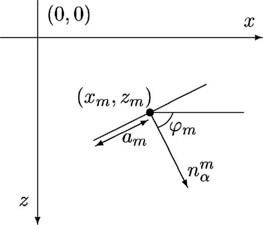
Each crack is represented by a line segment. It can be characterized by the position of its centre, x_m= (x_m, z_m), its half-width a_m and the angle ϕ_m with the horizontal. The z-coordinate indicates depth and the x-coordinate refers to the horizontal position. The unit vector normal to the crack is defined as n_α^m= (cos ϕ_m, sin ϕ_m).

Open in new tabDownload slide

In order to facilitate the derivation, we consider the frequency-domain form of the field quantities, indicated by . Later, we transform all of the resulting expressions back to the time domain. From the frequency-domain counterparts of eqs (1) and (2), we can eliminate the stress tensor and obtain

5

where the wave operator is defined by

6

Now, we decompose the total field into the incident and scattered field:

7

7

By definition, the incident field, which would be present in the absence of the cracks, satisfies the equation

9

The scattered field satisfies the source-free wave equation away from the cracks:

10

and the boundary condition

11

The scattered field satisfies the following integral representation (Van den Berg 1982):

12

in which is the particle displacement jump across the mth crack and is the Green stress tensor, defined by

13

The function is the elastic Green displacement tensor of the embedding medium. It satisfies the elastodynamic wave equation for a point source, i.e.

14

where δ is the Dirac delta distribution and δ_αη is the Kronecker delta. This study is restricted to small-scale cracks, i.e. the size of the cracks is small compared with the scale on which the wavefield varies. If the cracks are small enough, we can neglect the variation of the Green stress tensor during the integration over each crack, leading to

15

where x_m is the coordinate vector of the crack centre and x′ is the coordinate along the crack. Applying the wave operator , given by eq. (6), to both sides of eq. (15), yields

16

where the tensor g_αν^m follows from eqs (13) and (15) as

17

Since the Green tensor is, by definition, the solution of the elastic wave equation for a point source, eq. (14), we can express the tensor g_αν^m directly in terms of dipole-like point sources in the following way:

18

and therefore we can interpret g_αν^m as the point-source tensor. From eqs (16) and (18), we see that the explicit boundary conditions at the cracks now have been replaced by secondary point sources at the crack locations. Of course, in order to compute the secondary source strengths at the cracks, the boundary conditions still have to be imposed. An integral-equation formulation for the source strengths can be obtained from eq. (12), letting the point of observation approach the cracks and applying the boundary condition (4). However, this approach is impractical for heterogeneous media because computing the Green function can be computationally very expensive. Therefore, we approach the problem in a different way by approximating the source strengths with the aid of perturbation theory and using an FD formulation for computing the solution of eq. (16). Perturbation theory leads to an approximate source strength (Van den Berg 1982) in terms of the stress tensor of the incident field:

19

The derivation, as well as expressions for , are given in Appendix A. This approximation is based upon the following assumptions.

• Second- and higher-order scattering effects, i.e. the interactions between the different cracks, are neglected.

• The crack size is small compared with the wavelength of the incident wave. This implies that the incident wave is considered to be locally plane at the location of the crack and that the source strength can be approximated by the leading-order term in a perturbation series (see also De Hoop 1955a, b). We also neglect variations of the embedding medium in the direct vicinity of the crack.

The first assumption is the most restrictive one in our case. In principle, it can be relaxed by taking higher-order terms into account in the Neumann-series expansion of (see also Muijres et al. 1998). It is not straightforward, however, to discretize these higher-order terms with sufficient accuracy when using the FD scheme.

The time-domain form of eq. (9), required for FD formulations, is given by

20

with the time-domain wave operator L_αγ given by

21

From eqs (16) and (19), we can now derive a similar equation for the scattered field:

22

with the secondary source term s_α^sc given by

23

Expressions for P_νβ^m are given in Appendix A, see eqs (A20) and (A21). Since the crack location x_m does not coincide with a grid point, the incident field at x_m is computed using bilinear interpolation.

The scattering problem can now be solved using the FD method. First, the incident field is computed by solving eq. (20) for the (heterogeneous) embedding without accounting for the presence of the cracks; secondly, the (first-order) scattered field is obtained by solving eqs (22) and (23) with a similar technique. In this way, the problem of accounting for the explicit boundary conditions on many small cracks is avoided and replaced by the problem of accounting for the presence of many small point sources on an FD grid. This is discussed in the next section. In order to find a good representation of the dipole point sources occurring on the right-hand side of eq. (22), we need a representation of the wavefield in the direct vicinity of each crack. This is discussed in Appendix B, where expressions are also given for the discrete approximation of the collection of point sources present in s_α^sc of eq. (23).

3 Finite-difference method

We want to solve the elastic wave equation of the form

24

At each time step we solve this equation for two fields. For the incident field, we have

25

and for the scattered field, we use

26

A staggered FD scheme (Madariaga 1976; Virieux 1986) is used for the discretization of eq. (24). For the spatial discretization, grid points (x_i, z_j) are defined with x_i=x_min+iΔx and z_j=z_min+jΔz, where (x_min, z_min) are the coordinates of the upper left-hand corner of the grid. The displacement u₁ is shifted by half the grid spacing along the x-axis with respect to these grid points, and the vertical displacement u₃ is shifted by half the grid spacing along the z-axis:

27

28

Note that we have adopted a programmer's viewpoint in these definitions by using i and j in the superscripts rather than and . Time is discretized as t_n=t₀+nΔt. The quantities ρ_ij, λ_ij and μ_ij are all defined at (x_i, z_j). Below we will need ρ at (x_i+Δx, z_j). This quantity is denoted by ρ₍₁₎^i,j and computed using linear interpolation:

29

Likewise, we use

30

to obtain the density at (x_i, z_j+Δz). The quantity μ at the centre of a grid cell 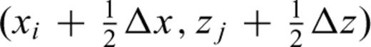is calculated by bilinear interpolation:

31

A typical staggered grid cell is shown in Fig. 2.

Figure 2

The staggered grid used in the FD method.

Open in new tabDownload slide

The elastic wave equation can be written as

32

33

The spatial derivatives are computed using the following standard central FD operators:

34

35

36

37

and similar definitions for u₃^i,j,n. These central differences D_x⁻ and D_z⁻ result in second-order accurate approximations of the derivatives of u₁ⁿ and u₃ⁿ at the points (x_i, z_j).

For the temporal discretization, a standard second-order FD scheme is used. The result is

38

and

39

For the computation of the scattered field, we have to distribute the point sources s_α^sc, given by eq. (23), over the grid points of the FD grid. This is discussed in Appendix B. We need a numerical representation of the point source that gives an accurate solution with the given second-order FD scheme. Following the approach of Van Baren et al. (2001), an accurate numerical approximation to the point source is constructed by applying the FD operator to the exact point-source solution. Instead of the exact solution, we use the asymptotic approximation to the scattered field given in eq. (15) which is valid close to the crack. Application of the numerical operator to this solution produces a numerical source term that is spread out over the grid points. Its amplitude decreases rapidly away from the position of the original point source. An example of a crack, represented by a distributed point source, is shown in Fig. 3. With this observation, we can simplify the expressions for the numerical source term by using approximations that are valid close to the crack.

Figure 3

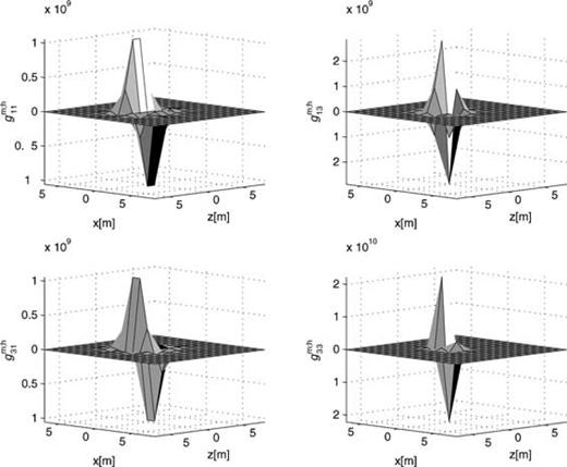
Discrete point-source tensor g_αν^m;h for one crack, computed using the staggered-grid FD operator. The crack is situated in the origin and is oriented along the x-axis. The half-width of the crack, a_m, is given by a_m= 0.5 m. The grid spacing is 2 m. The area around the crack, necessary to represent it as a distributed point source, is typically chosen as a square containing 7 × 7 grid cells.

Open in new tabDownload slide

4 Validation of the method

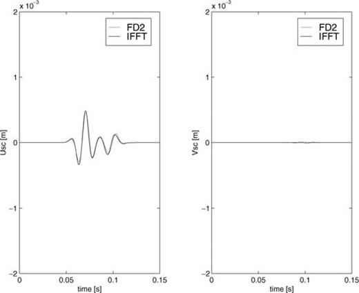
In order to validate our finite-difference method, we apply it to a single crack in a homogeneous embedding and compare its scattered wavefield with the scattered field resulting from a direct evaluation of the integral representation given in eq. (12) and transforming the result to the time domain. The latter method is not based on the discretization of the point-source tensor g_αν^m and therefore is a good validation test to check the accuracy of our method. For this comparison, we use an incident, plane, compressional wave propagating along the vertical axis. The waveform is a Ricker wavelet (second derivative of a Gaussian) with a dominant frequency of 45 Hz, corresponding to ω_c≈ 280 rad s⁻¹. The material parameters are chosen as: ρ= 2.3 × 10³ kg m⁻³, λ= 4.0 × 10⁹ N m⁻², μ= 5.2 × 10⁹ N m₋₂, which results in a compressional velocity c_p= 2.5 km s⁻¹ and a shear velocity c_s= 1.5 km s⁻¹. The compliant crack is situated at the origin (0, 0), parallel to the horizontal axis and has a half-width a_m= 0.5 m.For this choice of parameters, we have k_sa_m= 0.094 and k_pa_m= 0.057. Therefore, both values are much smaller than 1, which implies that the small-crack approximation is valid. The grid spacings Δx and Δz are both chosen to be equal to 2 m. In Figs 4–6, the horizontal and vertical components of the scattered displacement field in different directions are compared for both methods. The fit obtained is good, indicating that the discretization of the point-source tensor g_αν^m, represented by g_αν^m;h, is accurate. We have found that the discrete representation of the point-source tensor breaks down if the crack itself coincides with a grid point. This is a result of the singular behaviour of the point-source wavefield. For simulations with many cracks, we therefore have to discard cracks very close to grid points. In Fig. 7, we show snapshots of the scattered displacement field around the crack as computed with our method.

Figure 4

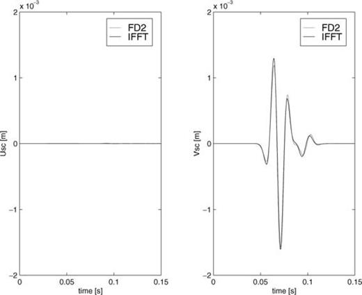
Horizontal and vertical components of the scattered displacement field observed in x= (0, −100). FD refers to our FD method and IR to the accurate integral-representation method. The field is normalized with respect to the incident field.

Open in new tabDownload slide

Figure 5

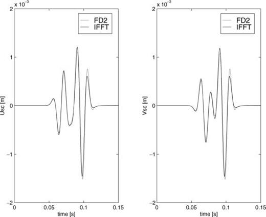
Same as in Fig. 4, but now observed in x = (70.7,−70.7).

Open in new tabDownload slide

Figure 6

Same as in Fig. 4, but now observed in x= (100, 0).

Open in new tabDownload slide

Figure 7

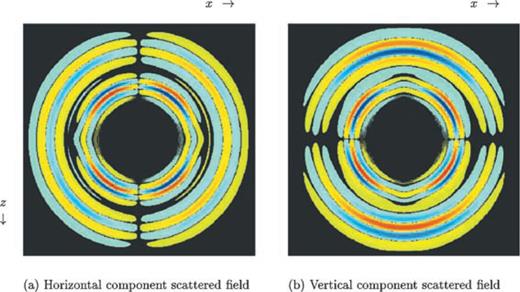
Snapshot of the horizontal and vertical components of the scattered displacement field for a vertically incident compressional wave on a compliant crack. The crack is parallel to the horizontal (x) axis and has a half-width a_m= 0.5 m.

Open in new tabDownload slide

5 Model study for a cross-well geometry

To illustrate the flexibility of our method, we simulate a cross-well experiment. The model consists of a low-velocity layer, containing 2000 small vertical cracks, situated between two high-velocity layers. The geometry of the experiment is shown in Fig. 8. The seismic source consists of a vertical point force and is situated in the low-velocity layer. In Fig. 9, we show snapshots of the horizontal and vertical components of the incident and scattered field. From the incident-field snapshots, we observe that a significant part of the wavefield is trapped within the low-velocity layer. The snapshots of the scattered field reveal two aspects. First, we see a coherent transmitted part. This is consistent with the concept of effective media (see, for instance, Hudson & Knopoff 1989), where the overall effect of the cracks is accounted for by an effective medium. Secondly, we observe that the backscattered field is much more complex, but nevertheless remains trapped in the low-velocity layer.

Figure 8

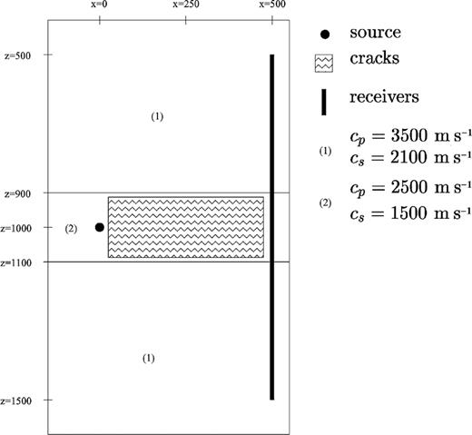
Cross-well geometry used in the example. The middle reservoir layer has a lower velocity than the upper and lower layers and consists of 2000 vertical cracks. The source is situated in the low-velocity layer.

Open in new tabDownload slide

Figure 9

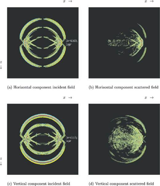
Snapshots of the horizontal and vertical components of the incident displacement field, that would be present in the absence of the cracks, and the displacement field scattered by the cracks. The model is shown in Fig. 8.

Open in new tabDownload slide

6 Discussion and conclusions

We have presented a finite-difference method for computing the scattering of 2-D, elastic waves by many small-scale compliant cracks, characterized by an explicit traction-free boundary condition. We have solved the problem of representing a small crack on an FD grid by deriving a suitable numerical source term. A further approximation of this source term provided a simpler expression that can be factored into a spatial and temporal part. This results in a substantial reduction of computing time, without an appreciable loss of accuracy. The most important limitation is a restriction to first-order scattering, which implies that interaction between cracks is not taken into account. This restriction could be alleviated by taking higher-order terms of the Neumann series into account. This extension, however, is not straightforward since it requires an accurate discretization of the scattered wavefield close to each crack.

We have included examples to validate the method and study the effect of the presence of 2000 small cracks in a low-velocity layer on the transmitted and reflected field. The strength of these effects depends on the number, size and orientation of the cracks.

The extension of the present method to three spatial dimensions is probably straightforward, provided the relevant perturbation expression is used for computing the secondary source strength from the incident field.

Appendix

Appendix A: The source strength in the case of a compliant crack

Without loss of generality, we assume the crack to be located at the origin. The half-width a_m of the crack is denoted by a. In order to use the results of Van den Berg (1982) directly, we use local coordinates for each crack such that the normal n_α, in local coordinates, is given by . In what follows, local quantities will be indicated with a tilde. At the end, we rotate all quantities back to the global coordinate system. The derivation can be found in more detail in Van den Berg (1982).

First, is approximated by a Chebyshev polynomial:

(A1)

Under the assumption that interaction between the cracks can be neglected, the coefficient d₁ satisfies the equation

(A2)

in which is defined by (see Van den Berg 1982)

(A3)

The Hankel function of the first kind and order one, H₁⁽¹⁾, is defined by H₁⁽¹⁾=J₁+iY₁. J₁ and Y₁ are the Bessel functions of the first and second kind, of order one, respectively. Furthermore, we have k_p=ω/c_p and k_s=ω/c_s (with angular frequency ω). The quantity can be calculated using the following series expansions of the Bessel functions (Watson 1944):

(A4)

(A5)

where Ψ is the logarithmic derivative of the gamma function, given by Ψ=Γ′/Γ. Because k_pa and k_sa are assumed to be small, we only take the first term of the summation into account. After tedious calculations, we find that

(A6)

The next step is to evaluate the integral on the left-hand side of eq. (A2). It is given by

(A7)

where we have used the fact that the strip is small compared with the dominant wavelength of the incident field. This allows us to replace the incident field by its value at the centre of the crack. If we substitute expressions (A6) and (A7) in eq. (A2), d₁ can be determined, and the source strength follows as

(A8)

The approximation of can be found in a similar way. Now, is approximated by a Chebyshev polynomial:

(A9)

The coefficient c₁ satisfies the equation

(A10)

in which is defined by (see Van den Berg 1982)

(A11)

The resulting source strength is

(A12)

So far, we have assumed that the crack was located at the origin. The source strength of a strip located at an arbitrary location x_m and with half-width a_m can now be written as

(A13)

with defined by

(A14)

(A15)

and

(A16)

If we restrict ourselves to the leading-order terms in k_pa_m and k_sa_m, and can be expressed as

(A17)

which implies that becomes real-valued and frequency-independent. With the aid of the coordinate transformation

(A18)

the quantities can be expressed in the global coordinates in the following way:

(A19)

with the global quantities expressed in the above local quantities by the relations:

(A20)

For small values of k_sa_m and k_pa_m (i.e. with the crack being small with respect to the wavelength), is real-valued and frequency-independent.

In order to compute the time-domain form, required for explicit time-domain FD techniques, we now transform the above expressions to the time domain. Since the frequency dependence of can be neglected for small values of the crack width a_m, see eqs (A16) and (A17), we can transform eq. (A19) directly to the time domain and obtain

(A21)

with given by eq. (A20).

Appendix

Appendix B: Accurate representation of point sources s_α^sc

We discuss the discrete representation of the point sources present in s_αsc of eq. (23). Since we consider only single scattering, we can treat each crack separately. First, we repeat eq. (22) for a single crack m in the frequency domain:

(B1)

with the source term being given by

(B2)

In the above equation, g_αν^m is a dipole-type point source at the crack location and is given by eq. (18). When we solve eq. (B1) with finite differences, we replace the exact operator by the operator after spatial discretization, which follows from eq. (6) as

(B3)

where Q_αγ^h is the discrete spatial differentiation operator. Since we evaluate it close to the crack, we can use the material parameters close to the crack and obtain

(B4)

where the second-order FD operators are given by

(B5)

and the first-order operators are defined in eqs (34)–(37). We express the discretized form of the scattered-field eq. (B1) in the following form:

(B6)

We now want to construct the source distribution resulting from the single crack by substituting the field close to the crack in eq. (B6) and evaluating the result.

Close to the crack, the scattered field follows from eq. (15) as

(B7)

If we now apply the discrete operator to both sides of eq. (B7), we obtain

(B8)

By inspection, we now find the discrete source term corresponding to the single crack to be given by

(B9)

or, equivalently, by

(B10)

where the discrete point-source tensor g_αν^m;h can be expressed in terms of the (known) FD operator and the Green tensor close to the crack:

(B11)

An example of this discrete point-source tensor is shown in Fig. 3. Close to the crack, the distance r (=|x−x′|) is small compared with the wavelength. This implies that we have and . Therefore, we can employ the leading-order term of the small-argument approximation of the Hankel functions present in . We obtain

(B12)

in which

To obtain the discrete point-source tensor g_αν^m;h, consider eq. (B11) and replace by its approximation close to the crack, given by eq. (B12). Close to the crack, the contribution of the spatial differentiation part (Q_αγh) of the operator is the largest owing to the singularity of the Hankel function. Therefore, we replace by its dominant spatial differentiation part, Q_αγ^h, and obtain

(B13)

with given by eq. (B4). Since the near-field form of the Green tensor is known explicitly, as well as the spatial part of the FD operator, Q_αγ^h, we can compute g_αν^m;h explicitly, by applying Q_αγ^h to .

We observe that the dominant part of g_αν^m;h does not depend on frequency. From eq. (B10), we now find that the time-domain form of the source term for the scattered field, s_α^sch, can be written as

(B14)

where we have also used eq. (A21). Since the crack location x_m does not coincide with a grid point, the incident field at x_m is computed using bilinear interpolation.

References