


Summary
Data from a new deep‐penetration seismic reflection line (LISA cruise 1995), onland seismic recording (LISA) and marine ESPs (expanding spread profiles, CROC II cruise 1981) are integrated to study the crustal structure of the north Ligurian basin. The correlation of these different seismic data, located along an Antibes–Ile Rousse transect, provides accurate information on the nature of the crust. On the Provençal margin, the multichannel seismic (MCS) profile LISA01 shows a major step in the basement. This structure is associated with a crustal change, corresponding to the ocean boundary. On the Corsica margin, we do not observe such a structure and the ocean boundary is constrained by magnetic anomalies. These anomalies are identical to those observed on the Provençal margin above the main basement structure. On the MCS line, the Messinian salt and the bottom water multiple obscure the crustal image below 7 s two‐way traveltime (TWTT). Nevertheless, the ESPs provide information about the crust below 7 s TWTT. These ESPs were reprocessed and analysed by matching traveltime and amplitude variations in the X–T and τ–p domains. The main result is the identification of a transitional zone on the continental margin (Provençal and Corsica margin) characterized by a layer with velocities of 7.2–7.3 km s−1 in the lower crust. Recordings from land stations on the Corsica margin define the geometry of this layer. In the centre of the basin, the oceanic crust is about 6 km thick. From the Corsica margin to the centre of the basin, the Moho depth decreases from 18 to 13 km. The velocity model deduced from offshore data is consistent with the ESP velocity model and MCS line LISA01. The combined analysis of these data allows us to propose a new boundary of the oceanic crust in the north Ligurian basin.
Introduction
The Liguro‐Provençal basin was formed by extension in a general geodynamic context of convergence between the African and European plates., This extensional phase since the Eocene (35 Ma) is considered to be a response to the subduction of Tethys under the European plate. The Liguro‐Provençal basin opened as a back‐arc basin since the middle Oligocene (30 Ma, Réhault 1981). The drifting phase was coeval with the anticlockwise rotation of the Corsica–Sardinia block ( Montigny . 1981 ) between 21 and 19 Ma ( Réhault 1981). The duration of the drifting phase is still controversial and the end of the rotation could be younger (15 Ma, Vigliotti & Langenheim 1995). The late Miocene and Quaternary post‐rift evolution of the Ligurian basin is characterized by a significant subsidence of the basin ( Réhault 1981). At present, the high level of seismicity of the basin shows compressional activity ( Béthoux . 1992 ), with an uplift of the margin with respect to the bottom of the basin ( Chaumillon . 1994 ).
The western Mediterranean Basin has been investigated using several geophysical methods: multichannel seismic profiles (MCS), two‐ship experiments (expanding spread profiles, ESP), heat flow measurements and aeromagnetic maps (see Gueguen 1995 for a recent review). However, some parts of the Mediterranean Basin are still poorly constrained because the backscattering and diffraction due to the Messinian salt diapirs obscure the seismic images and the seafloor multiple shadows the deep‐crustal seismic image. The Ligurian Sea, located in the northeastern corner of the Western Mediterranean Sea, is a particularly good example of an accumulation of geophysical data on the one hand and poor knowledge of the deep structure on the other. However, this area is crucial for reconstructing the plate tectonics of the entire basin because a good definition of the ocean boundary (OB) is necessary to define the initial fit. Moreover, the width of the domain where the oceanic crust has been emplaced during the early Miocene opening will constrain the initial position of Sardinia, which is more distant from the rotational pole than Corsica and has consequently undergone larger drifting.
To improve our geophysical knowledge of the Mediterranean Sea, the MCS LISA cruise was carried out in 1995. A single‐bubble airgun array and a 96‐channel streamer were towed at 20 m depth to obtain low frequencies and deep penetration ( Avedik . 1993 ). In the Ligurian Sea, the first profile was selected to image the geophysical transect of the ESP previously studied by Le Douaran . (1984) . The shots of the MCS line were recorded onland in Provençe and Corsica to obtain wide‐angle reflection and refraction data on the same transect. Other ESPs in the Provençal basin have been reprocessed and correlated with the coincident ECORS deep‐penetrating MCS profile ( Pascal . 1993 ). This approach has been quite successful and the final results differ significantly from the first study ( Le Douaran . 1984 ). The ESP Ligurian transect has been used in numerous publications ( Burrus 1984; Pasquale . 1993, 1994, 1996; Gueguen 1995) but never reanalysed, whereas the other geophysical data (heat flow, magnetic and gravimetric) in the Mediterranean Sea are regularly re‐examined and criticized ( Pasquale . 1993, 1996; Mendel 1993; Chamot‐Rooke . 1997 ).
Data acquisition
The data used in this study include four ESPs, the LISA multichannel seismic reflection lines, onland recording of the LISA shots and some industrial seismic reflection lines. The MS47 MCS profile from Offici Geofisica Sperimentale (OGS) of Trieste ( Finetti & Morelli 1973) and the Augusta 4 line of IFP (Institut Français du Pétrole) ( Réhault 1981) were particularly useful ( Fig. 1).
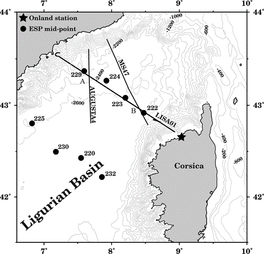
Location map of the north Ligurian basin and of the data used in this study. Contours are of bathymetry every 200 m. LISA01 is divided in two parts: LISA01‐A on the Provençal margin with ESPs 229 and 224, and LISA01‐B on the Corsica margin with ESPs 223 and 222.
Expanding spread profile acquisition
The initial objective of this study was to find the velocity structure under the Messinian salt of this region. The shooting ship in the 1981 ESP experiment was equipped with a 651 000 in3 airgun array and the recording ship towed a 2.5 km long streamer with 48 channels ( Le Douaran . 1984 ). An ESP experiment is a multiple‐fold wide‐angle reflection/refraction data set acquired by two ships steaming apart from a common midpoint, one shooting and the other one recording ( Fig. 2; Stoffa & Buhl 1979). In this experiment the two ships started from initial positions 65 km apart at the endpoint of each ESP profile, moved towards each other crossing a midpoint at a separation of less than 1 km and moved away steaming on reciprocal tracks at a constant speed of 5.4 knots. A common fixed central reference point was maintained to reduce the effects of dipping interfaces on determining interval velocities ( Diebold & Stoffa 1981). Two profiles are obtained, one at approaching ranges and one at departing ranges. Only one profile is used for the interpretation.
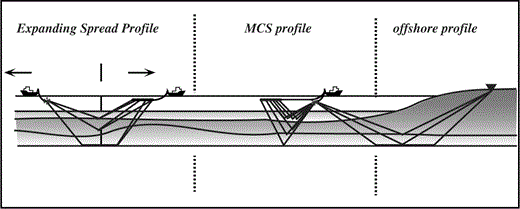
Sketches of the various ship configurations and the onland seismic station used during the experiment.
Multichannel seismic data from the LISA cruise
The multichannel seismic data were acquired during the LISA cruise (1995). The aim of the cruise was to image the crustal structure along the Antibes–Ile Rousse transect by using a low‐frequency source. 10 Generator‐Injector airguns used in ‘single bubble mode’ provided the seismic source. In this operational mode the signature of the 10 airguns is synchronized on the first bubble pulse instead of the initial spike, thus generating a low‐frequency and energetic signal ( Avedik . 1993 ). The distance between the shots was 55 m. A 2400 m long, 96‐channel streamer recorded the airgun array over a window of 15 s with a sampling rate of 4 ms. The offset between the seismic source and the head of the streamer was 310 m. This acquisition geometry provided a 12.5 m interval between each common midpoint with a 24‐fold coverage.
Onland recording of the LISA shot
During the LISA cruise some seismic stations were emplaced onland in Nice (by the Laboratoire de Geodynamique de Nice–Sophia Antipolis team) and on Cap Corse (by the Laboratoire de Sismologie Experimentale team of IPGP). On the continental side, the recording stations were Reftek recorders. On Corsica the stations were Lennartz M88 and 5800. Arrayed in this configuration, the offset between the station and ship changed as the ship moved away from or approached the stations ( Fig. 2). The stations were in‐line with the offshore profile ( Fig. 1). The shot interval was 21.5 s, long enough to avoid perturbation of the record by the previous shot.
Data processing
Expanding spread profile processing
The processing for X–T sections was as follows: stack at common offset to increase the signal‐to‐noise ratio; frequency filter to remove high‐ and low‐frequency noise; F–K filter to remove the dipping noise corresponding to velocities lower than 1.5 km s−1 and negative velocities. The τ–p section was obtained from the X–T section by using the generalized Radon transform ( Henry . 1980 ; Chapman 1981). The different steps of the processing were made using the Geovecteur software at the Ecole Normale Supérieure de Paris.
To construct the velocity model in the X–T and τ–p domains we use the ray‐tracing software jdseis ( Diebold & Stoffa 1981), kindly provided by J. Diebold. All interpretations were made with a 1‐D model, as the structure below the ESPs is laterally quite homogeneous. The velocity model was built layer by layer, minimizing the difference between the observed and calculated traveltimes. With the jdseis software the calculated traveltimes are directly superimposed upon real data. This visualization avoids the picking stage and picking errors and facilitates the identification of each phase. The main source of error arises from the poor correlation of phases due to the interference between reflected and refracted waves. Consequently, particular care was taken in identifying the different phases.
A waveform amplitude modelling was then performed to constrain the velocity model better, taking into account the contribution of P and S waves in the X–T and τ–p domains. The synthetic seismograms in the X–T domain were computed with the reflectivity method ( Kennett 1974; Vera . 1990 ). The computation was again carried out in a 1‐D model. To reproduce the real data, the medium response is convolved with a source wavelet with an average frequency of 20 Hz. The synthetic seismogram in the τ–p domain was also computed in 1‐D models with an algorithm developed by Dietrich (1988).
The old processing and interpretation of these ESPs did not take into account wide‐angle reflections, only the refracted phases. Furthermore, no synthetic seismogram was performed. Another important point is that there was no MCS line on these ESPs in the first interpretation. This is why the LISA01 MCS line was carried out.
Multichannel seismic data processing
The LISA data set was processed at the Ecole et Observatoire de Physique du Globe (EOPG) of Strasbourg. In the North Ligurian basin, poor seismic data quality results mainly from the presence of Messinian salt, which produces backscattering and diffraction of the signal. Moreover, the shallow water produces multiple reflections of the seafloor and of the sedimentary cover that are superimposed on the primary reflection deeper than 6 s TWTT in the deep basin. To reduce this effect we tested several methods of multiple attenuation. The best solution was obtained by subtracting a synthetic trace of the multiple from the initial trace. This modelled trace corresponds to the initial trace shifted by a time corresponding to the sea bottom. This pre‐stack step was applied to a common midpoint (CMP) gather in a conventional processing flow using the Geovecteur software.
The processing flow consisted of reading the data from 0 to 12 s, editing noisy traces, dynamic equalization according to depth, bandpass filtering according to depth, F–K filtering on each shot gather to eliminate dipping noise, multiple attenuation, spike deconvolution, bandpass filtering according to depth to remove high‐frequency noise generated by the spike deconvolution, trace sorting in common depth point (CDP), muting of traces to remove the noise of the water layer, velocity analysis, normal moveout (NMO) correction, 24‐fold addition of the traces and post‐stack migration in time in the F–K domain.
Onland recording processing
The velocity model derived from forward modelling of wide‐angle reflection/refraction data is not constrained by reverse shots. Nevertheless, we can propose velocity models where the geometry of the superficial layers is constrained by the MCS reflection profile (here LISA01) and the deep part is constrained by the onland recording. Therefore, we used the ESP velocity models to constrain the wide‐angle reflection/refraction model.
The velocity model is built by minimizing the difference between observed traveltimes and calculated traveltimes obtained by the ray tracing method of Zelt & Smith (1992). As for ESPs, the calculated traveltimes are interactively superimposed on real data. The direct method is used to construct the velocity model because of the reduced number of receivers. Additionally, a vertical time section of the model is calculated and superimposed on the MCS line to verify the coherence of the velocity model.
The mcs line lisa 01 antibes–ile rousse transect
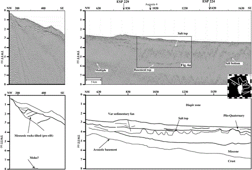
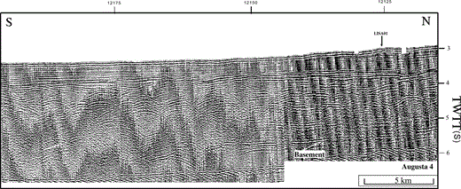
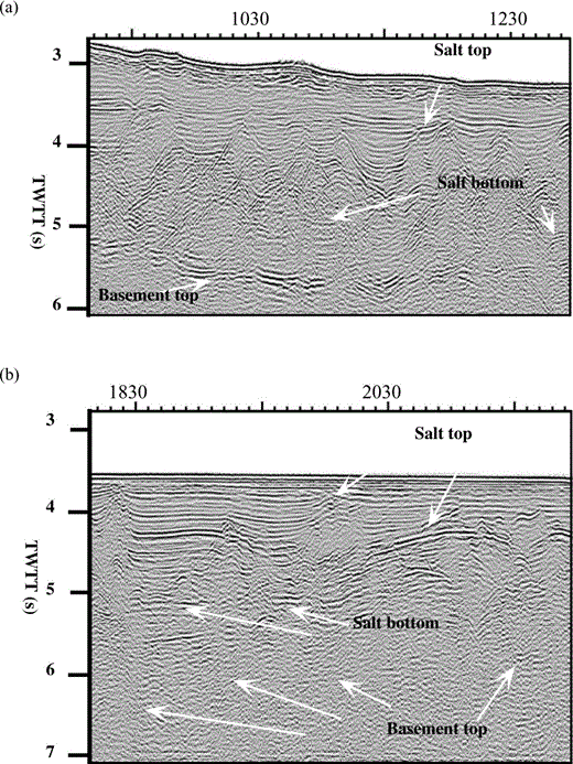
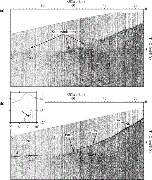
The quality of this seismic profile is quite variable and we were not able to improve the quality of the information significantly in the central area where diffractions generated by the salt diapirs dissipate the seismic energy. MCS line LISA01 is divided into two parts, LISA01‐A on the Provençal margin on ESPs 229 and 224 ( Fig. 3), and LISA01‐B on ESPs 223 and 222 on the Corsica margin ( Fig. 5). The sedimentary layer was very well described in previous work ( Réhault 1981). This sedimentary section can be divided into an upper Pliocene–Quaternary layer, a middle Messinian evaporitic and salt layer and a lower Miocene layer. Off Antibes, parallel landward‐dipping layers are underlain by a listric fault. These layers are probably Mesozoic rocks tilted during the Oligocene–early Miocene rifting of the Ligurian Sea ( Fig. 3). The western part of the LISA 01 MCS line shows a flat and highly reflective acoustic basement that deepens to more than 6 s TWTT and whose seismic character disappears at shotpoint 1230 (Figs 3 and 6a). This kind of basement has also been observed on the Augusta 4 seismic profile ( Réhault 1981; Fig. 4). In the central part of the Ligurian Sea, where the basement is deeper than 6 s TWTT, the first step can be seen at shotpoint 1900 (Figs 5 and 6b), although the basement is poorly imaged. After the second step at shotpoint 2100, the basement is shallower than 6 s TWTT. The acoustic basement is poorly imaged except in the southeastern part of the Ligurian Sea, where some clear reflections are visible (shotpoint 2630). The Corsica margin is steep and some deep horizons, at 7 and 8 s TWTT ( Fig. 5), may correspond to lower crust and Moho reflections.
LISA01 MCS profile, Provençal margin. The quality of the profile is disturbed by the presence of salt and by the multiple arriving around 7 s TWTT. Nevertheless, the top of the basement is visible between shotpoints 830 and 1230. The processing flow consisted of reading of the data from 0 to 12 s, editing noisy traces, dynamic equalization according to depth, bandpass filtering according to depth, F–K filtering on each shot gather to eliminate dipping noise, multiple attenuation, spike deconvolution, bandpass filtering according to depth to remove high‐frequency noise generated by the spike deconvolution, trace sorting in CDP, muting of traces to remove the noise of the water layer; velocity analysis, NMO correction, addition of the traces with a 24 fold addition, and post‐stack migration in time in the F–K domain.
LISA01 MCS profile, Corsica margin. The quality of the profile is also disturbed by the presence of salt and by the multiple arriving around 7 s TWTT. On the Corsica margin we do not observe a prominent reflector like that on the Provençal margin. The processing flow consisted of reading of the data from 0 to 12 s, editing noisy traces, dynamic equalization according to depth, bandpass filtering according to depth, F–K filtering on each shot gather to eliminate dipping noise, multiple attenuation, spike deconvolution, bandpass filtering according to depth to remove high‐frequency noise generated by the spike deconvolution, trace sorting in CDP, muting of traces to remove the noise of the water layer, velocity analysis, NMO correction, addition of the traces with a 24 fold addition, and post‐stack migration in time in the F–K domain.

Seismic profile Augusta 4; see Fig. 1 for location. This profile shows an acoustic basement similar to the basement observed on the LISA01 MCS profile. This non‐migrated profile comes from Réhault (1981) and was acquired by IFP (Institut Français du Pétrole).
The previous interpretation of the ESPs was based on the seismic profile MS47 carried out by an Italian institute, OGS ( Finetti & Morelli 1973). The basement map originally in seconds ( Réhault 1981) was recomputed in metres ( Chamot‐Rooke . 1997 ). Seismic profile MS47 images a basement ridge (Tristanite Ridge) that is mapped in the centre of the Ligurian Sea ( Fig. 7a). The basement of this ridge crops out towards the northeast and a basalt sample was dredged. This basalt, 18 Myr old, is similar to the volcanic rock of Tristan Da Cunha, an island located on the South Atlantic spreading centre ( Réhault 1981). This Tristanite ridge was interpreted as the fossil spreading centre of the Ligurian Sea formed at the end of the rotation of the Corsica–Sardinia block ( Réhault 1981). The oceanic origin of this basement high was subsequently debated in several studies ( Burrus 1984; Pasquale . 1993, 1994, 1996; Gueguen 1995) and the northeastern end of this ridge is currently interpreted as a volcanic high in a continental setting ( Chamot‐Rooke . 1997 ). According to the depth‐to‐basement map ( Fig. 7a) the acoustic basement at shotpoint 2100 on LISA 01 should be less than 5 s TWTT deep. However, the depth is actually at about 6 s TWTT; consequently there is no basement high on LISA 01 ( Fig. 7b) and the ridge detected on the MS 47 ( Fig. 7c) does not extend continuously towards the southwest. This observation has very important consequences: southwest of LISA 01 there is no ridge in the oceanic domain and a fracture zone may separate the basement high seen on MS 47 (northeast of LISA 1) and the deep basement observed on LISA 01.
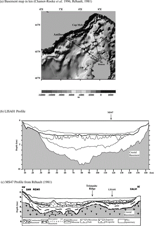
(a) Basement map in km ( Chamot‐Rooke . 1996; Réhault 1981), where the LISA01 basement is not included, and locations of the different profiles. On the MCS line LISA01 (b) there is no basement high, as observed on seismic line MS47 (c). A fracture zone may separate the basement high seen on MS47 and the deep basement observed on the LISA01 MCS line.
Expanding spread profile
These ESPs were shot in a NE–SW direction that parallels the strike of the basement slope. Therefore, this situation is favourable for the ESP records. However, the northern branch of ESP 223 is located on the basement high seen on MS 47 and the southern branch is in the deep basin. Nevertheless, the records of all the ESPs, including ESP 223, are of good quality. The structure of the basement and the thickness of the sedimentary section observed at the intersection of the ESPs and LISA 01 have been used for the construction of the velocity model. The intersection with LISA 01 corresponds to the common midpoint of the ESPs, except ESP 224, which is slightly offset to the northeast.
Esp 229
The recomputed velocity model is presented in Table 1. On the X–T section ( Fig. 8a), beneath the seafloor reflection (Rfd), the reflection Rpq corresponds to a 0.83 km thick layer of Pliocene–Quaternary sediments with a velocity of 2 km s−1. At the base of this layer a refracted wave (re) corresponds to a velocity of 3.8–4 km s−1. This second layer, 1.67 km thick, is formed by Messinian evaporites undeformed by salt diapirism. Beneath the Messinian evaporites a 1.93 km thick Miocene layer has a velocity of 4.4 km s−1. These phases are well constrained in the X–T ( Fig. 8a) and τ–p ( Fig. 8c) domains. The strong energy observed between 19 and 23 km can be attributed to the critical distance of the basement arrivals. Between 18 and 50 km, refracted arrivals are observed. The first refracted arrival, rc1, corresponds to a 2.39 km thick layer with a velocity of 4.8 km s−1. The top of this layer corresponds to the acoustic basement identified on the MCS profile ( Fig. 6a). The second refracted arrival, rc2, is related to a 1 km thick layer with a velocity of 5.2 km s−1. A third phase, rc3, corresponds to a 1.96 km thick layer with a velocity of 6.3 km s−1. A wide‐angle reflected wave on the Moho, named Rpmp, is overlain by a 2.22 km thick layer with a velocity of 7.2 km s−1. The deep layers are poorly imaged in the τ–p domain and rc2, rc3 and Rpmp cannot be identified. The synthetic seismogram ( Fig. 8b) in the X–T domain shows the focusing of the energy at 10, 20 and 27 km. Arrival rpn is related to the Moho at 14 km depth.
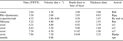
Velocity model ESP229. r: refractors; R: reflectors.
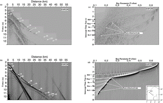
X–T and τ–p section of ESP229. (a) Observed record section with the main phases. (b) Synthetic seismogram for the final velocity model presented in Table 1 with the main phases. (c) Observed record section with the main phases. (d) Synthetic seismogram for the final velocity model presented in Table 1 with the main phases.
Esp 224
The final model is presented in Table 2. On the X–T ( Fig. 9a) section, Re2 is associated with a prominent increase of energy observed at a distance of 12 km. This Re2 phase corresponds in the τ–p domain ( Fig. 9c) to an inflection located at 4 s TWTT and 0.25 s km−1. Re2 is related to a 1.45 km thick layer of Messinian evaporites and salt, with a velocity between 3.75 and 4 km s−1. The 4.45 km s−1 velocity is associated with a 1.7 km thick Miocene (Rm) layer. rc1 and rc2 are clearly identified in the X–T domain but poorly imaged in the τ–p domain because salt diapirism disturbs the seismic section. The first phase, rc1, is associated with a 1.5 km thick layer with a velocity of 5 km s−1. The second, rc2, corresponds to a 2.7 km thick layer with a velocity of 6.3 km s−1. The Moho (rpn) is identified at a depth of 13.3 km.
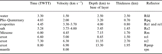
Velocity model ESP224. r: refractors; R: reflectors.
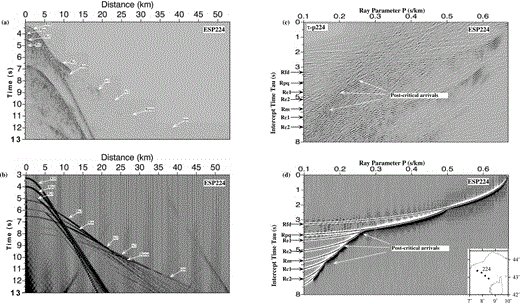
X–T and τ–p section of ESP224. (a) Observed record section with the main phases. (b) Synthetic seismogram for the final velocity model presented in Table 2 with the main phases. (c) Observed record section with the main phases. (d) Synthetic seismogram for the final velocity model presented in Table 2 with the main phases.
Esp 223
The final model is presented in Table 3. After the seafloor reflection (Rfd), the 0.4 km thick Pliocene Quaternary layer (Rpq) is associated with a compressional velocity of 2 km s−1 ( Fig. 10a). The refracted arrival (re1) from the top of the Messinian evaporites is clearly evident. This layer is 1.11 km thick and the velocity varies from 3.15 to 3.63 km s−1. Below the evaporites, Re2 is a reflected wave corresponding to a 1.66 km thick Messinian salt layer with a velocity of 3.9 km s−1. The Miocene layer is 1.08 km thick and has a velocity of 4.5 km s−1. The acoustic basement has been previously identified on the MCS profile ( Fig. 5). The refracted arrivals in the crust are shown in the X–T ( Fig. 10a) and τ–p ( Fig. 10c) domains. rc1 corresponds to a 1.29 km thick layer with a velocity of 5.2 km s−1. This layer is underlain by a 2.31 km thick layer with a velocity of 6 km s−1. Rpmp corresponds to the reflected arrival from the Moho. The rpn phase is related to a Moho at 12.55 km depth. The synthetic seismogram in the X–T domain shows the concentration of energy located at 15, 20 and 25 km ( Fig. 10b).
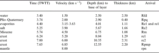
Velocity model ESP223. r: refractors; R: reflectors.
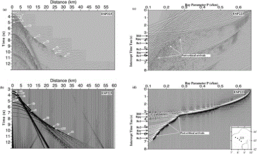
X–T and τ–p section of ESP223. (a) Observed record section with the main phases. (b) Synthetic seismogram for the final velocity model presented in Table 3 with the main phases. (c) Observed record section with the main phases. (d) Synthetic seismogram for the final velocity model presented in Table 3 with the main phases.
Esp 222
The final model is presented in Table 4. The Messinian salt disturbs this ESP. In the X–T domain ( Fig. 11a), after the reflections on the sea bottom (Rfd) and on the Pliocene–Quaternary (Rpq), a branch, re1, ends at a distance of 8 km. This phase is associated with a 0.93 km thick layer with a velocity gradient increasing from 3.71 to 4.45 km s−1. Below this high‐velocity layer a 1.17 km thick layer (Re2) corresponds to a low velocity between 3.64 and 3.82 km s−1. This inversion of velocity is probably produced by a Messinian salt lens extruded onto the Pliocene Quaternary sedimentary cover. This inversion can be seen in the X–T ( Fig. 11a) and τ–p ( Fig. 11c) domains. The Miocene layer (Rm) is 1.53 km thick and has a velocity of 4.5 km s−1. At offsets greater than 15 km, crustal arrivals are observed. rc1 is refracted at the top of the basement and corresponds to a 2.09 km thick layer with a velocity of 5.4 km s−1. The second arrival, rc2, is associated with a 2.52 km thick layer with a velocity of 6.17 km s−1. The Rpmp phase corresponds to a reflection from the Moho overlain by a 2.98 km thick layer with a velocity of 7.3 km s−1. A 14 km depth for the Moho is given by the refracted wave, rpn. The crust is 7.6 km thick. The synthetic seismogram ( Fig. 11b) shows the good fit with different observed phases and the inversion of velocity at a distance of 8 km. The energy focused at 15 km corresponds to the critical distance for the basement arrivals.

Velocity model ESP222. r: refractors; R: reflectors.
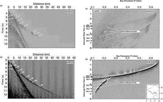
X–T and τ–p section of ESP222. (a) Observed record section with the main phases. (b) Synthetic seismogram for the final velocity model presented in Table 4 with the main phases. (c) Observed record section with the main phases. (d) Synthetic seismogram for the final velocity model presented in Table 4 with the main phases.
Onland recording
On the MCS line LISA 01, the salt diapirs dissipate the energy by diffraction and prevent good penetration. Moreover, the seafloor multiple is located at 7 s TWTT, which conceals the deep structure. To obtain some information on the deep crust and particularly on the geometry of the Moho, the shots were recorded by land stations in the area of Nice and in Corsica. The records in the first region are noisy but the wide‐angle reflection and refraction data are very good in Corsica. The distance ranges from 15 to 100 km. The original records are presented with a reduction velocity of 8 km s−1 and are corrected for bathymetry to facilitate the identification of each phase ( Fig. 12a). The undulations in the arrivals are caused by the salt diapirism.
Onland recording of the LISA profile. (a) Onland recording represented using a velocity reduction of 8 km s−1 and a correction of the bathymetric effect. From 45 to 100 km, undulations caused by the salt are observed. (b) Onland recording represented using a velocity reduction of 8 km s−1 and the main phases. The black lines represent the traveltime calculated with the final model from Fig. 13(a).
Pso corresponds to the refracted wave from the basement and Pci is related to the refracted arrival on the lower crust ( Fig. 12b). PmP and Pn are the reflected and refracted arrivals from the Moho, respectively ( Fig. 12b). A model ( Fig. 13) was constructed by ray tracing with the constraints of the ESP results and MCS line LISA 1. The thickness of the Pliocene/Quaternary layer (velocity 2.1 km s−1) varies from 0 on the Corsica slope to 1 km in the basin. The second layer has a velocity of 2.5–4.5 km s−1. This layer, which is formed by the Messinian evaporites and by the underlying Miocene, is thin on the Corsica slope and up to 4 km thick in the basin. The upper crustal layer is modelled with two gradients. At a distance of 15 km from the station, the velocity varies from 5.4 to 5.5 km s−1. The low velocity (4.5 km s−1) is imposed by the Pso phase corresponding to the refracted waves from the basement. This low velocity may be attributed to the weathering of the Hercynian granite that crops out at the Ile Rousse. The refracted arrivals Pci are associated with a 2–5 km thick layer that yields a velocity of 6.3–6.4 km s−1. This layer is well constrained by the ESP results. To model the lower crust we took into account the strong lateral velocity changes between ESPs 222 and 223. At large offset the 7.2–7.3 km s−1 layer disappears and is replaced by a 6.8–6.9 km s−1 layer. Several velocity layer geometries were tested by the study of the PmP delay between 30 and 65 km from the recording station. The best fit is obtained when the 7.2–7.3 km s−1 layer thins progressively away from the station and disappears at 70 km from the station. Its maximum thickness is 3 km at a distance of 30 km from the station. After 70 km the Pn arrival needs the introduction of a velocity lower than 7 km s−1. The thickness of this 6.8–6.9 km s−1 layer varies from 0 at 70 km to 2.5 km at 100 km from the recording station.
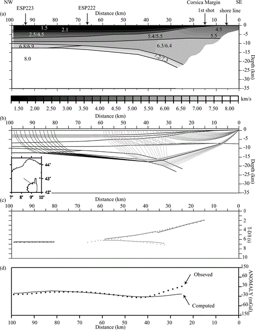
(a) Final velocity model obtained from the analysis of onland recording. (b) Ray sampling of the model. (c) Comparison of calculated (lines) and observed (dots) traveltimes. (d) Gravity modelling from the velocity model in (a). The misfit between observed and calculated data is due to the low ray coverage at the southeastern boundary of the velocity model and to the bad quality of Sandwell's data near the coast.
The Moho is 20 km deep at a distance of 30 km from the station and 12.5 km deep at 100 km. To take into account the PmP arrival it is necessary to introduce a prominent shallowing of the crust–mantle boundary at 35 km from the station. The Moho depth at a distance of more than 80 km is determined by the Pn phase. Beneath the station previous refraction studies ( Hirn & Sapin 1976) indicate that the Moho is 30 km deep.
Gravity modelling was also performed using the algorithm of Talwani . (1959) for polygonal volumes with an infinite lateral extension ( Fig. 13d) and using Sandwell .'s (1995) free‐air anomaly data. There is a good fit between the computed and observed data in the basin. The misfit between observed and calculated data is due to the low ray coverage at the southeastern boundary of the velocity model and to the bad quality of Sandwell's data near the coast.
To test the model we calculated the corresponding reflection time at vertical incidence and we superimposed this time model on the MCS profile LISA 01 ( Fig. 14). The model is coherent with the MCS line as well as with the ESP results.
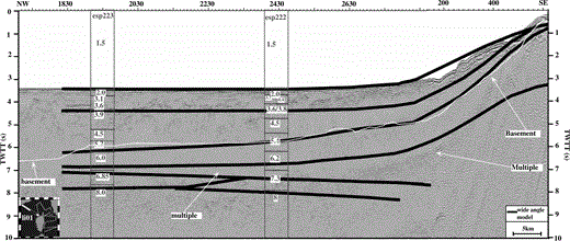
Eastern part of the LISA01 MCS profile. Boundaries from the wide‐angle velocity model and two ESP velocity models are superimposed on the MCS line.
Discussion
(i)Differences between our velocity model, deduced from ESP data and the Le Douaran . (1984) velocity model
The previous interpretation ( Le Douaran . 1984 ) was based on the ESP refracted arrivals and the information on the sedimentary cover was derived from a non‐coincident seismic profile (MS 47). Our reprocessing introduces the wide‐angle reflections and we calculate synthetic seismograms in the X–T and τ–p domains. Moreover, the acoustic basement, that is, the top of the crust, was determined on the LISA 01 seismic profile, which is coincident with the midpoint of the ESPs.
In ESP 229 the top of the crust was higher (about 4 km depth) than in the MS 47 results, and included a 4.4 km s−1 layer that could also be interpreted as pre‐rift sediments ( Fig. 15) ( Le Douaran . 1984 ). In our interpretation the acoustic basement of LISA 01 is much deeper (about 6 km depth). It is flat and shows a low velocity (4.8 km s−1), which suggests a sedimentary composition such as Mesozoic carbonates included in the acoustic basement. However, the real basement cannot be much deeper than the basement at ESP 229 and consequently the 4.8 km s−1 layer is not completely sedimentary. The identification of the 7.2 km s−1 layer, at the base of the crust, is an important new result and is characteristic of rifted crust.

Comparison between the crustal section obtain in this study (a) with the crustal section of Le Douaran . (1984) (b). Numbers indicate compressional wave velocities (km s−1). Locations of ESPs are indicated by their common central points.
In ESP 224 the basement was previously assumed to be oceanic with a two‐layer division ( Fig. 15b). However, a 6 km s−1 velocity is too low for lower oceanic crust ( White . 1992 ). In our model the lower crust has a velocity of 6.9 km s−1 in good agreement with the structure of the oceanic crust deduced from ESP data.
In ESP 223 the 3.6–4.1 km s−1 layer was previously associated with a volcanic feature and the top of the crust (4.5 km s−1) was higher, as shown by the MS 47 seismic profile (about 6 km depth). In our interpretation the top of the solid crust (5.2 km s−1) is lower and the LISA 01 seismic profile does not show any evidence of a basement high (about 7 km depth). The Moho velocity is much too high (8.9 km s−1) in the Le Douaran . (1984) model ( Fig. 15b).
In ESP 222 the acoustic basement is shallower on MS 47 than on LISA 01 and thus the top of the solid crust (5.4 km s−1) is deeper (6.4 km) in our interpretation than in Le Douran's study (4.9 km s−1 and 4.8 km deep) ( Fig. 15). We find evidence for a velocity inversion related to the Messinian salt and a lower crust with a high velocity (7.3 km s−1).
In summary, the depth to the Moho is not significantly different in the two interpretations, but the crust is much thinner and has a different velocity structure in our interpretation than in Le Douaran's interpretation.
(ii)Seismic velocity structure and nature of the crust
The study of a non‐volcanic continental margin shows that seismically it is difficult to discriminate between an oceanic crust and a thinned continental crust because neither the velocity nor the thickness are characteristic of one type of crust. However, the velocities of typical oceanic crust ( White . 1984 ; White . 1992 ) and of thinned continental crust ( Whitmarsh . 1986 ) are now well known. Between the two types of crust there may be an ocean–continent transition zone ( Discovery 215 Working Group 1998).
We compare our results with those of the Gulf of Lion ( Pascal . 1993 ). ESPs 215 and 216 are located in the oceanic domain of the Gulf of Lion, and the shaded area in Fig. 16 represents the velocity structure of 50–170 Myr Atlantic oceanic crust ( White . 1984, 1992). On the other hand, ESP 203 was located at the boundary between the continental crust and the ocean–continent transition zone (Pascal . 1993). This transition zone is about 150 km wide and is characterized by lower crust with a velocity of 7.2–7.4 km s−1 ( Pascal . 1993 ). ESPs 229 and 222 shows the same crustal structure with velocities of 7.2–7.3 km s−1 ( Fig. 16). The onland records on the Corsica margin constrain the geometry of this layer.
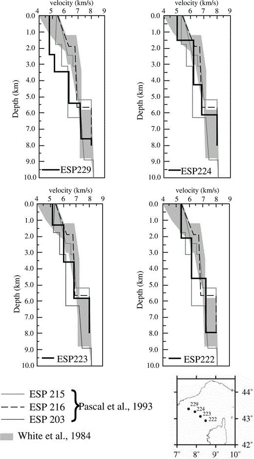
The velocity–depth profiles of the ESPs with respect to reference oceanic crust and transitional crust models based on synthetic seismogram modelling. The oceanic crust reference is represented by ESP 215, ESP 216 ( Pascal . 1993) and the envelope of 50–170 North Atlantic models in grey (White . 1984). ESP 203 represents the reference for the transitional crust (Pascal . 1993).
The most quoted hypothesis for the formation of this high‐velocity layer is the serpentinization of the upper mantle exhumed during rifting ( Boillot . 1989 ; Discovery 215 Working Group 1998). If the mantle was initially at the top of the 7.2–7.3 km s−1 layer, then the Moho moved downwards by hydration and serpentinization of the peridotites. This situation has already been observed on other margins, including the Galicia Bank ( Whitmarsh . 1996 ; Boillot . 1995 ), the southern Iberia abyssal plain ( Discovery 215 Working Group 1998) and Tagus abyssal plain ( Pinheiro . 1992 ) margins, and the Newfoundland ( Reid 1994) and Labrador and Greenland conjugate margins ( Chian . 1995 ). On the Galicia Bank, the velocities of the serpentinized peridotite ridge vary from 7.4 to 7.8 km s−1, and the crustal thickness (upper and lower crust) over this ridge varies from 2 to 5 km with velocities from 5.2 to 6.8 km s−1 ( Whitmarsh . 1996 ). On the Ligurian (Corsica and Provençal) margins, the velocities of the crust vary from 4.8 to 6.3 km s−1 with a thickness from 4.5 to 5 km (ESPs 222 and 229). The thickness of the crust above the high‐velocity lower crust is in the same range as is observed on the Galicia Bank, except on the most necked parts (about 2 km thick, Whitmarsh . 1996 ). As a consequence, the thickness of the upper transitional crust of the Ligurian margins may allow the hydration of the peridotites. The geometric differences of the serpentinized peridotite bodies between the two margins could come from the more homogeneous stretching in the North Ligurian Basin than on the Galicia Bank. Moreover, we have to take into account the fact that we have used only ESPs, which give us a 1‐D high‐resolution velocity model, and just one onland seismic station, which limits our knowledge of the geometry of crustal layers. Furthermore, no exhumed mantle has been drilled on the Ligurian Margin. Makris . (1999) also observed a unit in the lower crust with a velocity of 7.2–7.5 km s−1 in the Gulf of Genoa. They proposed underplating of mantle material, emplaced prior to the onset of seafloor spreading, to explain this high‐velocity zone. However, in that area the upper crust above the high‐velocity layer is about 15 km thick, preventing any serpentinization of the peridotites. We do not know if this high‐velocity layer can be followed laterally into the north of the Ligurian Sea because of a lack of deep seismic data in this area. We thus favour the hypothesis of serpentinized peridotites to explain the existence of the high‐velocity layer in the North Ligurian Sea.
In the model of ESP 224 the high velocity disappears and is replaced by a lower velocity (6.9 km s−1) characteristic of the lower oceanic crust ( White . 1984, 1992). The same velocity (6.85 km s−1) was also determined on ESP 223. These two ESPs have a velocity structure very similar to those of ESPs 215 and 216 located in the Provençal Basin, where oceanic crust has been identified ( Pascal . 1993 ). Therefore, we consider that ESPs 224 and 223 are located in the oceanic domain of the Ligurian Sea. The oceanic crust is about 5–6 km thick, slightly less than the thickness of normal oceanic crust (7 km, White . 1984, 1992). This thickness is also observed in the Gulf of Lion (about 5.5 km, Pascal . 1993 ) and in the Gulf of Genoa (6–7 km, Makris . 1999 ). ESP 224 was supposedly located in the oceanic domain, whereas continental crust was assumed by Le Douaran . (1984) beneath the ESP 223. We show that ESPs 224 and 223 are both representative of the oceanic crust and that ESPs 229 and 222 are located in the transition zones and thinned continental crust that lie in the deep margins of Provençe and Corsica, respectively.
On the Corsica Margin, the original thickness of the crust was 30 km with a velocity from 6 to 6.5 km s−1 ( Béthoux . 1999 ). In the basin, we observe velocities of 5.4 and 6.17 km s−1 for the 4.5 km thick crust over the anomalous velocity of 7.3 km s−1 (ESP 222). On the Provençal margin, the original thickness of the crust was also 30 km with velocity from 5.8 to 6.2 km s−1 ( Fontaine 1996). On ESP 229, on the Provençal Margin, we find velocities in the 5.5 km thick crust from 4.8 to 6.3 km s−1, overlying a 7.2 km s−1 layer. On both ESPs, we find some velocities lower than the adjacent velocities observed on the unthinned crust. In the transition zones of the Southwest Greenland ( Chian . 1995 ) and Labrador ( Chian & Louden 1994) Margins, a low‐velocity crust (4–5 km s−1 on the Southwest Greenland Margin and 4.8–5 km s−1 on the Labrador Margin) was found above a high‐velocity lower crust (7.2–7.5 km s−1 on the Southwest Greenland Margin and 6.4–7.7 km s−1 on the Labrador Margin). The nature of the low‐velocity upper crust, continental or oceanic, in this transitional zone is always a subject of discussion. The velocities that we find in the upper crust are higher than the velocities found on the Labrador Sea margins, but also lower than the velocity observed on the adjacent continental crust. The presence of 6.3 and 6.17 km s−1 velocities just above the high‐velocity lower crust may suggest a continental affinity.
(iii)Boundaries of the oceanic crust
The boundaries of oceanic crust are located between ESPs 229 and 224 on the Provençal side and between ESPs 223 and 222 on the Corsica side. On ESP 229, a flat reflector, observed on the MCS line LISA01, corresponds to the acoustic basement in the continental domain (Figs 3 and 6a). An important boundary in the nature of the crust cannot be placed where the reflector can be followed without interruption. The flat reflector loses its reflectivity near shotpoint 1200 (Figs 3 and 6a) where the acoustic basement deepens in the direction of the basin centre. This step is also perceptible on the Augusta 4 seismic profile before shotpoint 12 175 ( Fig. 4) in the same direction. On the aeromagnetic map reduced to the pole ( Mendel 1993) ( Fig. 17) this step and the disappearance of the flat reflector correspond to a steep gradient between a low and the central relatively positive magnetic anomaly. Therefore, we place the boundary of the oceanic crust on the Provençal side along this gradient. The boundary on the Corsica side is placed by analogy along a gradient in the aeromagnetic map and a step in the basement at shotpoint 2100 on seismic profile LISA 01, although this feature and the acoustic basement are less evident on this side of the Ligurian Sea. The boundary may be obscured by the volcanic edifice shown in the magnetic map and MCS profile MS47 ( Fig. 6c), which is north of seismic profile LISA01.
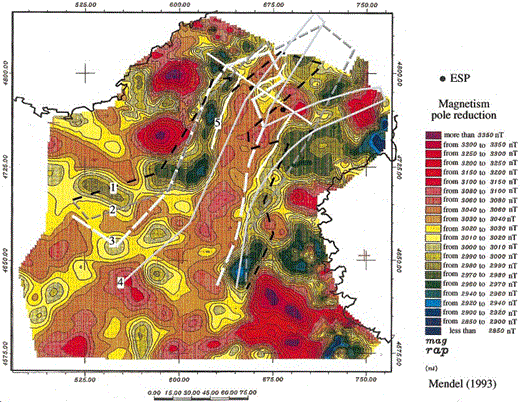
Magnetic map ( Mendel 1993) with different ocean boundaries proposed by several authors in the north Ligurian basin. (1) Pasquale . 1996); (2) Réhault (1981); (3) Burrus (1984); (4) Gueguen (1995); (5) the ocean boundary proposed in this study. A fracture zone may separate the basement high seen on MS47 and the deep basement observed on the LISA01 MCS line. This fracture zone is characterized by a shift of the magnetic anomalies on the magnetic map.
Fig. 17 shows different positions of the ocean boundary ( Burrus 1984; Pasquale . 1993, 1994, 1996; Gueguen 1995) and our interpretation. A fracture zone between the MS 47 and LISA 01 seismic profiles may explain the deepening of the acoustic basement between the northern continental domain and the southern oceanic zone. This fracture zone also explains the offset of the oceanic domain in the northern part of the Ligurian Sea and the difference between the relatively broad south Provençal margin and the narrow north margin (Figs 6b and c).
(iv)Provençal–Corsica transect
Previous interpretations ( Chamot‐Rooke . 1997 ; Le Douaran . 1984 ) and our new crustal transect are presented in Fig. 18(b). The Moho depth has been obtained ( Chamot‐Rooke . 1997 ) by inversion of the gravity data and from these results it was inferred that the crust, which is very thick beneath ESP 222, is continental along the Antibes–Ile Rousse transect. However, the basement depth of the Réhault (1981) study ( Fig. 7a) has been used for this inversion and again the high of the MS 47 seismic profile ( Fig. 7c, i.e. the Tristanite ridge) and the proximity of the thick crust under Corsica disturb the results.
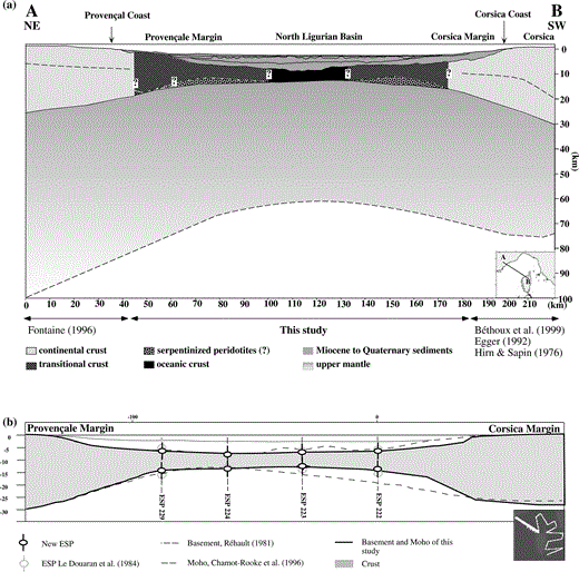
(a) Crustal and lithospheric section proposed in this study integrated with published data. On the Provençal margin the crustal structure is constrained by the study of Fontaine (1996). The lithospheric depth is given by Panza & Suhadolc 1990) along the transect. On the Western Corsica margin several authors give the crustal structure (Béthoux . 1999; Egger 1992; Hirn & Sapin 1976). (b) Comparison between the different studies made along this transect and our study for the Moho and basement depths.
In our model the oceanic crust is 6 km thick beneath ESPs 223 and 224, and 4 km thick in the centre of the basin, which is thicker than in the previous models. The thickening of the crust beneath each margin is abrupt and more or less symmetrical in our model. However, an asymmetry between the Corsica and Provençal margins is generally postulated ( Réhault 1981; Réhault . 1984 ; Jemsek . 1985 ; Pasquale . 1993, 1994, 1996; Gueguen 1995). Constraints on the Provençal margin are lacking to establish the real geometry of the thickening of the continental crust.
The northern boundary of the Ligurian oceanic crust is relatively well determined by seismic data along the Cap Mele–Cap Corse fracture zone ( Fig. 17) ( Béthoux . 1986 ; Réhault 1981; Réhault . 1984 ). The mantle beneath the Gulf of Genoa, investigated during the European Geophysical Transect, has a surprisingly low velocity (7.4–7.7 km s−1) ( Egger 1992; Ginzburg . 1986 ). Such low velocities are also found in the Tyrrhenian Sea and the Gulf of Genoa, which have been affected by recent rifting, as attested by high heat flow.
In the southern part of the Ligurian Sea (on ESPs 225, 230, 220 and 232; see Fig. 1 for location), the thickness of the oceanic crust (less than 4 km) is less ( Le Douaran . 1984 ) than the 6 km determined for ESPs 224 and 223 and about 4 km in the centre of the basin ( Fig. 15a). Normal oceanic crust is 7 ± 1 km thick when the spreading centre is a permanent feature ( White . 1992 ). In the south of the Ligurian Sea where the oceanic domain is wider, the thickness of the oceanic crust should be greater ( Chamot‐Rooke . 1996 ; Bown & White 1994). In fact, in the southern part the rate of spreading is larger and the crust is more extended than in the northern part, where the oceanic domain is restricted and the rate of accretion is lower because of the proximity of the pole of rotation ( Chamot‐Rooke . 1997 ). However, the crustal structure of the ESP in the southern Ligurian basin should be studied again with the techniques applied in this work since the crustal thickness may be wrong in the previous study ( Le Douaran . 1984 ).
As in the Provençal basin ( de Voogd . 1991 ), we do not find evidence of a spreading centre in the Ligurian Sea, although a trough between ESPs 224 and 223 is observed on the LISA 01 seismic profile ( Fig. 15a). This absence of topographic expression may suggest rapid accretion. Such rapid accretion (about 40 mm yr−1 full rate) was assumed in the previous interpretation ( Montigny . 1981 ; Réhault 1981) where the emplacement of oceanic crust was brief (21–19 Ma). However, the timing of the end of the rotation of the Sardinia–Corsica block is still doubtful ( Vigliotti & Langenheim 1995).
Conclusions
The combined analysis of the four ESPs, the almost coincident MCS line LISA 01 and the data from land stations provide detailed information on the crustal structure of the north Ligurian basin. The ESPs were reprocessed and analysed by matching traveltime and amplitude variations in the X–T and τ–p domains. The resulting crustal section has a transitional crust on the continental margin (Provençal and Corsica margins), characterized by a velocity layer of 7.2–7.3 km s−1 in the lower crust, interpreted as serpentinized peridotites. The upper crust of this transitional zone shows velocities of continental affinity. Arrivals at a land station, on the Corsica margin, define the geometry of the high‐velocity lower crust layer. The oceanic crust in the centre of the basin is about 6 km thick. From the Corsica margin to the centre of the basin, there is a decrease of the Moho depth from 18 to 13 km.
On the Provençal side, the multichannel seismic profile shows the main structure in the basement. This structure is associated with a change in the nature of the crust corresponding to the ocean boundary. On the Corsica margin, the ocean boundary is fixed by magnetic anomalies. These anomalies are identical to the anomalies observed on the Provençal margin above the main basement structure.
The combined analysis of these data allows us to propose a new boundary of the oceanic crust in the north Ligurian basin. This domain contains a fracture zone not described previously.
Acknowledgments
We thank the editor, K. E. Louden and J. B. Diebold for constructive reviews, which helped to improve the manuscript. We thank Elf for providing the ESP magnetic tapes and Ifremer for giving us a copy of the ESP navigation. We thank David Lemeur for helping us to use jdseis software. We are grateful to Nicolas Chamot‐Rooke, who provided the basement map of the Ligurian Sea, for his helpful suggestions.
Now at: IUEM, Place Copernic 29280 Plouzané, France. E‐mail: [email protected]
References
