The effects on seismic waves of interconnected nearly aligned cracks

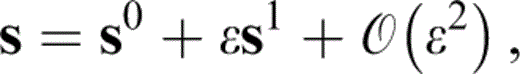
SUMMARY

Transfer of fluid between connected cracks may occur during the passage of seismic waves. Such fluid flow can be modelled using an extension of effective medium theory (Hudson 1996) and is effected via non‐compliant pores. The flow is governed by a parameter τ representing the relaxation time of pressure equalization between cracks. However, if the cracks are fully aligned and have the same aspect ratio, the theory produces the unexpected result that, at low frequencies, the cracks are effectively isolated and at high frequencies they are fully drained. The artificial restriction of the model to perfectly aligned cracks of identical aspect ratio is seen to be the cause of this result. By reworking the model to allow the crack orientation and aspect ratios to vary, we see that a more realistic model has the usual properties in which the cracks are isolated at high frequencies and undrained at low frequencies. We have chosen the distributions of aspect ratios to be in agreement with observation (Hay 1988) . Thomsen's parameters (Thomsen 1986) and the attenuation coefficients are seen to be frequency‐dependent via the non‐dimensional parameter Ωτ.

1 INTRODUCTION

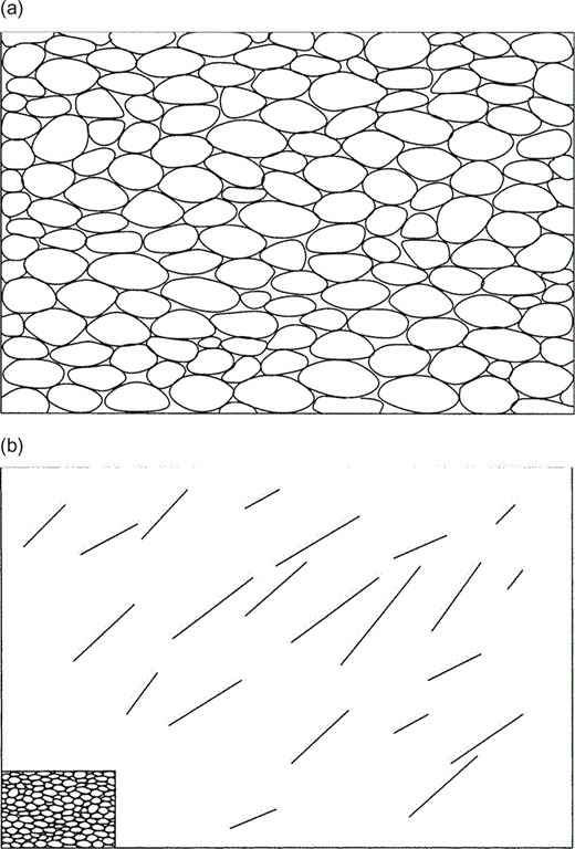
Cracking originates in rocks from a number of geological processes, of which thermal gradients and tectonic stress are particularly important. The resulting fracture network will depend upon both the mineralogy and grain orientation within the rock. Experiments on thermally induced cracking (Fredrich & Wong 1986; Hadley 1976; Homand‐Etienne & Houpert 1989) and stress‐induced cracking (Montoto 1995, Tapponnier & Brace 1976, Wong 1982) suggest that the former process produces a fairly isotropic distribution of predominantly intergranular cracks, while the latter produces a strongly anisotropic distribution of intragranular and transgranular cracks, with the majority of cracks oriented parallel to the direction of maximum principal stress (David 1999; Menéndez 1999).

Effective medium theories giving expressions for the overall mechanical properties (in particular, the wave speeds) of materials with cracks are now well established. Among the best known are the self‐consistent method ( O’Connell & Budiansky 1974), the method of smoothing ( Hudson 1980) and the differential method ( Nishizawa 1982). In all such theories it is necessary to calculate the response of a single crack in an unbounded homogeneous matrix. Since all the methods involve extensive averaging, the cracks are represented for this purpose by a ‘mean crack’, usually taken to be circular. The cracks may be aligned, partially aligned or randomly oriented ( Hudson 1986), they may be filled with gas (dry), liquid or a weak solid ( Hudson 1981) and they may be connected through the porosity of the matrix rock (Hudson 1996; O’Connell & Budiansky 1977). In the latter case, fluid is able to flow between cracks that, because of their difference in orientation, say, have been distorted differently by an imposed stress field. We follow the analysis of Hudson (1996) here and it should be borne in mind that the theory developed here is valid only to first order in the number density of the cracks. Although Hudson (1996) and Pointer (2000) imply that the extension to second order in the number density is straightforward, it has not been established that this is the case and we restrict ourselves to a first‐order theory here.

In their paper, Hudson (1996) derived a rather unexpected result for aligned connected cracks. This was that, in high‐frequency wave propagation, the cracks behave as if they are completely drained (dry) and, at low frequencies, as if they are isolated without connections. Although apparently running against physical intuition, this result is explained by the fact that because the cracks are fully aligned, the pressure gradient driving fluid from one crack to another varies on the scale of a wavelength, inversely proportional to the frequency Ω; the diffusion length, on the other hand, varies as Ω^−1/2. Thus, as the frequency tends to zero, the diffusion is less and less effective, with the opposite effect as Ω→∞.

Hudson (1996) derived their results for aligned cracks by a method that ignores local crack‐to‐crack flow since it was assumed that because the cracks all have the same orientation, it would be unimportant. However, if the formulae for non‐aligned cracks are specialized to cracks with a single orientation, the result differs from the above in the addition of one term that becomes important at high frequencies. The incorporation of crack‐to‐crack flow shows that it cannot be neglected when the frequency is sufficiently high that the wavelength approaches the size of the intercrack spacing. We compare the two results here and show that, with the more complete theory, fully aligned cracks behave as if isolated at high frequencies as might be expected. However, they still behave as if isolated at very low frequencies for the reasons given above.

As well as depending on the assumption that the cracks are fully aligned, these results also rely on the fact that the cracks were assumed all to have the same aspect ratio. Relaxing either of these two assumptions leads to local fluid flow between neighbouring cracks that have been distorted in different ways by the incoming wave because of their different orientations or aspect ratios or both. In this paper we analyse the effect of allowing small variations in alignment and aspect ratio and find that the behaviour of the material is that of undrained cracks at low frequencies, in accordance with physical expectation. We show, graphically, how the material behaves when the cracks are nearly aligned and when they all have nearly the same aspect ratio.

2 BACKGROUND

The method of smoothing developed by Keller (1964) has been applied by Hudson (1980, 1981, 1986) to determine expressions for the effective elastic parameters c of a cracked material, to first order in crack density ε=ν^s〈a³〉, where ν^s=N/V, N is the number of cracks, V is the material volume, a is the crack radius and the operator 〈.〉 denotes the mean value, such that

where c⁰ is the elastic tensor for the assumed isotropic, porous matrix material,

where λ and μ are the Lamé constants of the material; c¹ accounts for scattering off individual cracks.

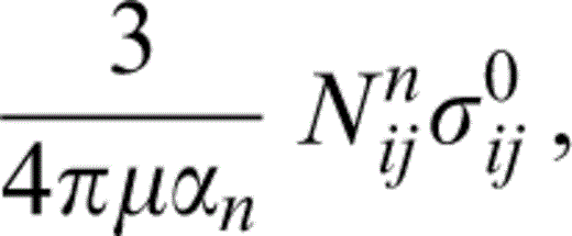
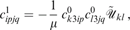
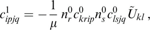
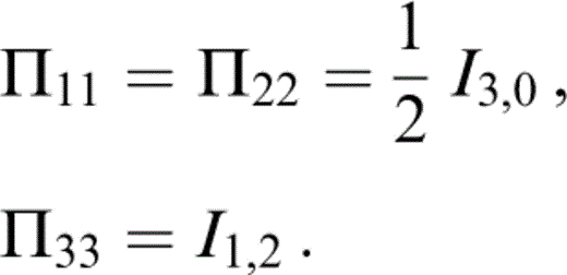
Determination of c¹ depends upon the orientation of the cracks and the nature of the crack infill. Expressions for c¹ under varying conditions for isolated cracks can be found in Hudson (1980, 1981, 1986). For aligned isolated cracks of identical aspect ratio, with normals lying in the x₃‐direction, these are of the form

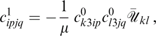
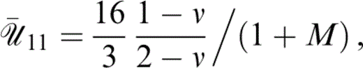
where the nature of the crack infill is reflected in the diagonal matrix {풰¯_kl}, where 풰¯₁₁=풰¯₂₂, due to the assumed symmetry of each crack. The resulting effective medium is vertically transversely isotropic.

3 THEORY

The model of connected cracks proposed by Hudson (1996) for the transfer of fluid between cracks by non‐compliant pores (seismically transparent pathways) (see Figs 1a and b) makes the assumptions that the distortion of the pores is negligible compared with that of the cracks during the passage of a wave and that the pore porosity is low, so that we neglect compression of the pore fluid.

The population of cracks is divided into families of parallel cracks with identical aspect ratio and identical radius, labelled n=1, 2, …. Hudson (1996) give a first‐order expression for the porosity of the nth set of cracks,

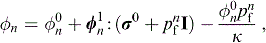
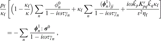
where κ=λ+2μ/3 is the bulk modulus of the matrix material, φ_n⁰ and φ_n¹ are the stress‐free porosity and the first‐order dependence on stress, respectively, for the nth set of cracks, σ⁰ is the imposed static stress field and p_fⁿ is the fluid pressure in the nth set of cracks.

The relation proposed by Hudson (1996) for the mass flow out of the nth set of cracks, derived in Appendix A, is

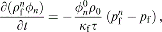
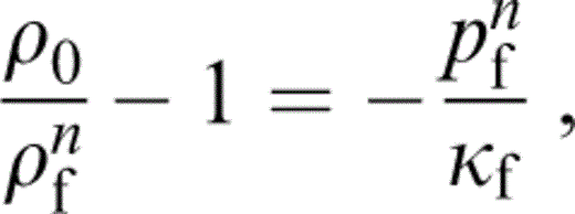
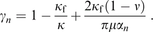
where ρ_fⁿ is the fluid density in the nth set of cracks, ρ₀ is the unstressed density, κ_f is the bulk modulus of the fluid, p_f is the average (local) pressure in the fluid and τ is a relaxation parameter. Estimations of the value of τ are made by Hudson (1996) and O’Connell & Budiansky (1977). This gives us the relationship between the fluid pressure, p_fⁿ, in the nth set of cracks, the average fluid pressure and the imposed static stress,

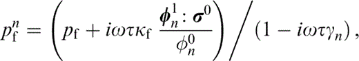
with

where we have used the relationship between the fluid pressure and density,

and have assumed a plane wave solution to the equations of motion of the form u=be^{i(k . x−Ωt)}, so that the operators ∂/∂x_i and ∂/∂t are replaced by the factors ik_i and −iΩ respectively. This is the opposite convention to that used by Hudson (1996) .

From Hudson (1996) , conservation of mass and D’Arcy's law yield an evolution equation for the total mass concentration of fluid, m_f,

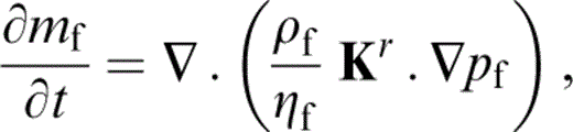
with K^r the permeability tensor of the matrix, including cracks—in general this will be anisotropic, although Hudson (1996) assumed an isotropic permeability; m_f is given by

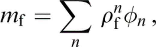
where ρ_f is the average fluid density, η_f is the fluid viscosity, and p_f and ρ_f obey the same relation as p_fⁿ and ρ_fⁿ in eq. (8).

Let us assume that K^r is spatially constant. Substituting eqs (4), (6) and (8) into eq. (10) and using eq. (9) we gain, to first order in p_f/κ_f and φ_n¹ : σ⁰/φ⁰, where φ⁰ is the average stress‐free porosity of the cracks,

where

is the ratio of the wavenumber in the x_i‐direction to the total wavenumber, and v is the wave speed; we approximate this to lowest order by using either v_P or v_S corresponding to P or S waves respectively.

Letting the normal to the nth set of cracks be nⁿ, from Hudson (1996) we have

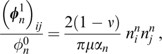
where α_n=c_n/a_n is the aspect ratio of the nth set of cracks and

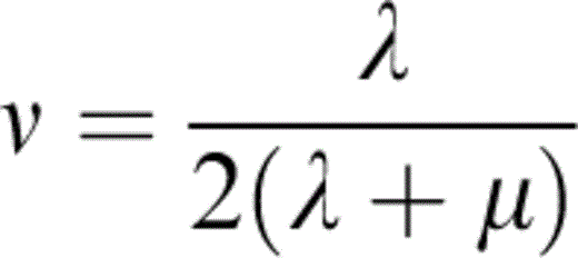
is Poisson's ratio of the matrix material. We now have

Substituting eq. (13) into eq. (11) yields an expression for p_f and hence by eq. (6) an expression for p_fⁿ in terms of σ⁰.

Thus, from eq. (4), the relative change in porosity becomes

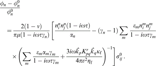
As in Hudson (1996) , we write this as

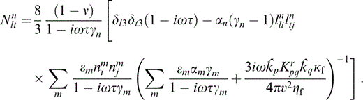
thus defining {N_ijⁿ}, the crack opening parameters for the nth set of cracks. This is a modified version of the corresponding result derived in Hudson (1996) that allows for variable aspect ratio.

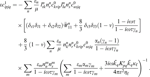
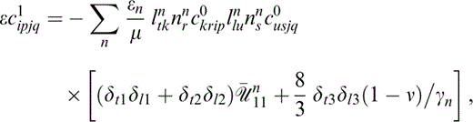
The analysis of Hudson (1996) now proceeds to show that the perturbation εc¹ in the elastic parameters is given by

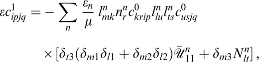
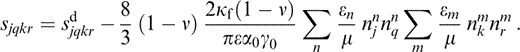
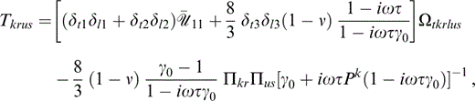
where ε_n is the crack density of the nth set of cracks; that is, ε_n=ν^s_na³_n, where ν^s_n is the number density and a_n is the radius of the nth set of cracks.

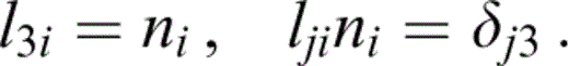
{l_ijⁿ} is the rotation matrix from the background axes to axes fixed in the crack with normal in the x₃‐direction, so that

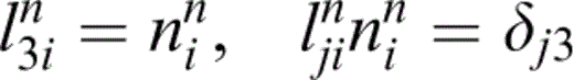
and we have adopted the opposite convention for the definition of {l_ijⁿ} to Hudson (1986), Hudson (1996) and Pointer (2000) . We note that Hudson (1996) incorrectly stated their choice of the sense of the rotation {l_ijⁿ}. The values of {N_ltⁿ} in eq. (18) are to be calculated for cracks with normals in the x₃‐direction,

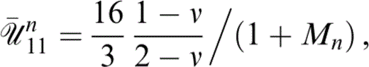
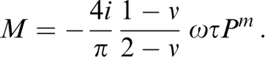
풰¯ⁿ₁₁ is given by Hudson (1981) for a weak viscous material infill with effective rigidity −iΩη_f as

where

Inserting eq. (20) into eq. (18), we finally arrive at an expression for the first‐order correction to the elastic constants,

4 HIGH‐ AND LOW‐FREQUENCY LIMITS

The behaviour of eq. (23) at high frequency is given by

which corresponds to the result for isolated cracks filled with a fluid with Ωη_f≪κ_f≪κ ( Hudson 1981); that is, a fluid such that its effective rigidity is small in relation to its bulk modulus, which in turn is negligible in comparison with the bulk modulus of the material. The low‐frequency limit of eq. (23) is

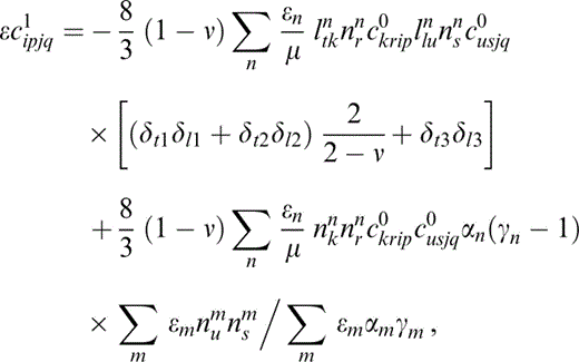
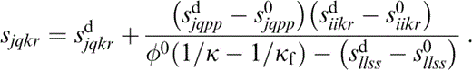
the first term of which corresponds to the result for dry cracks ( Hudson 1981). However, the presence of the second term means that the response at low frequencies is that for undrained material, as we now show.

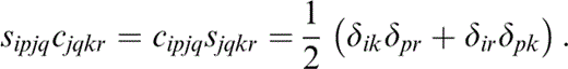
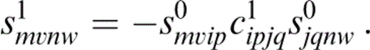
We define the compliances s in the same manner as we define the stiffnesses c (eq. 1), such that

where

and

Using the result in eq. (28) and assuming that eqs (1) and (26) represent power series, we equate the 풪(ε) terms and can therefore write s¹ in terms of c¹ as

Thus, for the low‐frequency limit,

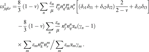
We write

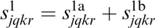
and identify s^1a and s^1b with the first and second terms of eq. (30) respectively. Thus, we may write the limit for dry cracks as

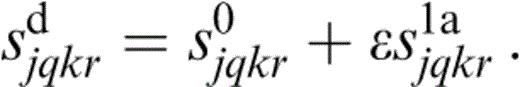
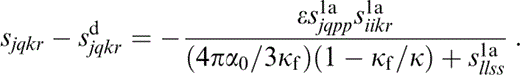
Brown & Korringa (1975) extended the work of Gassmann (1951) to give an expression for the undrained compliances in terms of the dry result,

Hence, from eq. (32) and using φ⁰=4πεα₀/3, where α₀=〈α〉,

From eq. (30),

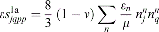
and

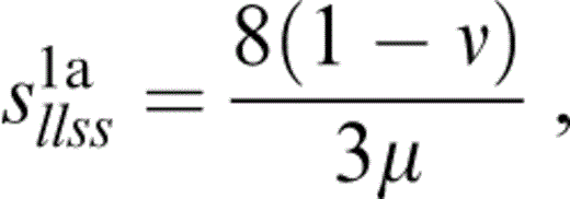
therefore eq. (34) becomes

where

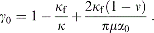
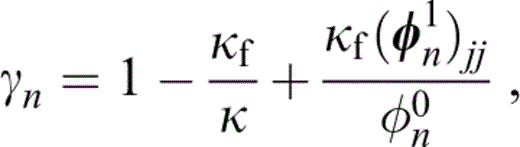
We note that Σ_m ε_m=ε and Σ_m ε_mα_m=εα₀, provided that we assume that ε and α are independently distributed parameters; then, from the definition of γ_m (eq. 15), Σ_m ε_mα_mγ_m=εα₀γ₀ and hence, from eq. (30),

We can neglect the term κ_f/κ in (γ_n−1) on the assumption that the maximum value of the aspect ratio, α_max, satisfies the condition

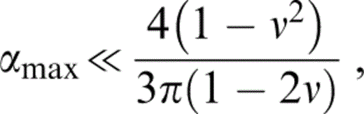
which is consistent with our restriction to small aspect ratios provided that ν?−1; then the term α_n(γ_n−1) in eq. (39) is independent of n, and eq. (39) reduces to the right‐hand side of eq. (37) exactly, so the undrained moduli are given by

This is identical to eq. (30) for the low‐frequency limit for connected cracks, showing that, at low frequencies, connected cracks respond at each point in exactly the same way as the same material under static, undrained conditions.

5 CONTINUOUS LIMIT

Having developed the theory from a discrete perspective, we shall henceforth assume a continuous limit: Σ_nF(n) in eq. (23) is replaced by

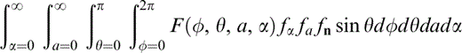
for any function F, where f_α, f_a and f_n are the probability distribution functions of the random variables α, a and n (defined by polar angles φ and θ) respectively. We shall assume that these distributions are independent of one another, for the purpose of separately assessing their effects on seismic anisotropy. More realistically perhaps, one would expect aspect ratio to depend upon orientation, with cracks parallel to the direction of maximum principal stress having a larger mean aspect ratio than those perpendicular to it. Gibson & Toksöz (1990) developed a model of a probability density function for crack orientation with an aspect ratio distribution included. Their results from the inversion of velocity measurements are generally good, although there is an implied non‐uniqueness of inversion.

Prior to the exposure to stress, a rock will have a generally isotropic background distribution of cracks ( David 1999) . Stress will induce further cracking, which will be of an anisotropic nature ( Menéndez 1999) , and thus a more accurate description of crack distributions within a rock may be obtained by representing the crack distribution as the sum of an isotropic and an anisotropic part.

For a given aspect ratio, the crack radius a_n only appears within the term ε_n in eq. (23), so that in the continuous limit it occurs in the form of 〈a³〉 only, and thus ε_n may be replaced everywhere by ε.

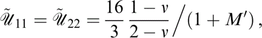
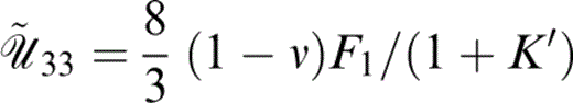
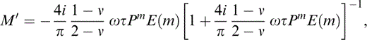
6 ALIGNED CRACKS

If we take the limit in which the cracks are fully aligned and of identical aspect ratio, we find that c¹ is given by eq. (3), with

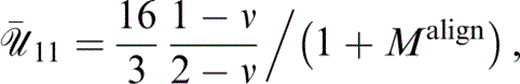
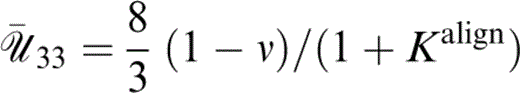
and

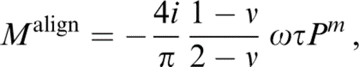
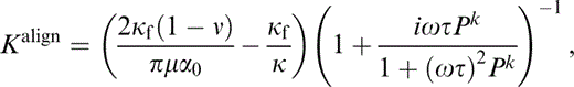
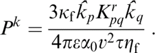
where

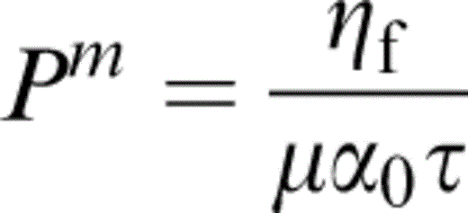
and

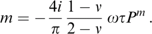
The quantity ΩτP^m is identical to the intracrack viscosity parameter P_v of Pointer (2000) , who estimated that, with the fluid properties of oil or water, its effect is negligible for seismological applications for both aligned and randomly oriented cracks.

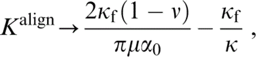
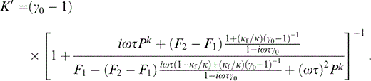
We have written the expressions in eqs (45) and (46) in terms of Ωτ, which is the short‐range diffusion parameter P_srd of Pointer (2000) and the quantity ΩτP^k is 3/4π times the long‐range diffusion parameter P_lrd of Pointer (2000) . Apart from the presence of an additional term—the κ_f/κ term, neglected by Hudson (1996) —this result is identical to the aligned limit of the expression derived for non‐aligned cracks by Hudson (1996) . Both of these expressions for aligned cracks with identical aspect ratio differ from that given by Hudson (1996) in the value of the parameter K^align; the formula given by Hudson (1996) is

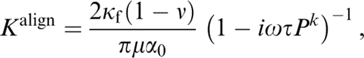
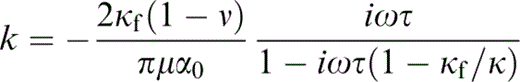
which ignores the term (Ωτ)²P^k and uses the opposite sign convention on the temporal derivative. This difference arises as a result of the failure of the aligned cracks result ( Hudson 1996) to account for any local fluid flow (note that ΩτP^k is independent of τ).

We see from eq. (46) that in either of the limits Ωτ→0 or Ωτ→∞,

which is the result for isolated cracks filled with a fluid with Ωn_f≪κ_f≪κ ( Hudson 1981). The inclusion of local crack‐to‐crack flow gives the expected result at high frequencies, but at very low frequencies the cracks still act as if isolated for the reasons given earlier.

7 VARIABLE ASPECT RATIO

To begin with, we assume that the cracks are fully aligned, hence

and consider the effects of variable aspect ratio only. Let us further assume that θ₀=0, so that all the cracks now have normals in the x₃‐direction. Eq. (23) now takes a form identical to that of eq. (3),

where {풰˜_ij} is a diagonal matrix with

and

We have defined here two functions that depend upon the probability distribution function of α,

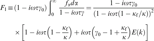
and

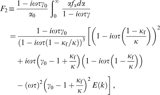
where

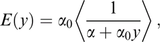
and the parameters of the distribution are chosen such that 〈α〉=α₀. Finally,

and

We can generalize this result to the case of arbitrary values of θ₀ and φ₀, letting the normal to the cracks be n⁰=(sin θ₀ cos φ₀, sin θ₀ sin φ₀, cos θ₀)^T,

where {Ũ_ij} is just the rotation of {풰˜_ij} to the new axes and is given by

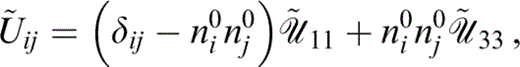
with 풰˜₁₁ and 풰˜₃₃ given as above (eqs 53 and 54).

7.1Modelling the distribution

Our theory restricts us to consider α≪1 only, so we look for distributions with a finite range and a small mean. For this we have chosen a generalized form of the Beta distribution ( e.g. Ross 1989), Beta(u, p, q), with a probability density function (pdf)

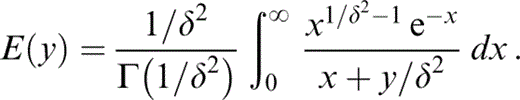
and B(x, y) is the Beta function ( e.g. Carrier 1983) . The three parameters p, q and u allow us considerable flexibility with our model and in particular we may choose them such that the pdf closely resembles observational results ( Hay 1988) .

We wish to fit the parameters of the distribution such that

for some δ. Thus we choose p and q such that

Our choice of δ will dictate the spread of the distribution and u=α_max, the maximum value of α that can be achieved.

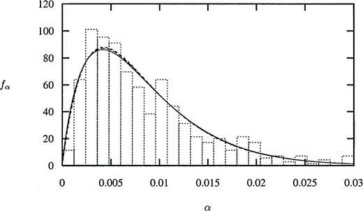
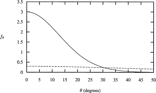
Choosing u=0.2, α₀=0.00837 and δ=0.703 ensures that our probability density function resembles the results of Hay (1988) (see Fig. 2) based upon a truncation of the data provided in Hay (1988), where the larger aspect ratio values have been ignored. For α greater than some critical value much less than u, the pdf is effectively zero; it is not surprising, therefore, that variations in u have a negligible effect upon the values of the elastic constants—while there is a very small observable difference between the Beta distribution with u=0.2 and 0.5 ( Fig. 2), there is no discernible difference between the resulting components of the stiffnesses (eq. 52)—so we replace eq. (64) with

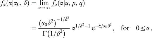
which is a Gamma(1/δ², 1/α₀δ²) distribution ( Ross 1989), with Γ(z) the Gamma function ( Carrier 1983) . Graphically, this looks almost identical to the Beta distribution with u=0.5 ( Fig. 2). With this choice of distribution, we have

7.2 Results

We start by choosing the parameters of the Gamma distribution such that it closely follows the measurements of Hay (1988) ; thus α₀=0.00837 and δ=0.703. Furthermore, we shall use ε=0.02, v_P=3.5×10³ m s⁻¹, v_S=2.0×10³ m s⁻¹ and ρ=2.2×10³ kg m⁻³ (average values that could correspond to a large number of possible matrix materials), κ_f=2.25×10⁹ Pa and η_f=10⁻³ Pa s (for water), thus ν=0.258 and κ_f/κ=0.148. We shall, for simplicity, assume that {K^r_pq}=K^rδ_pq and use K^r=10³ mD (≃10⁻¹² m²), so that only the parameter τ remains unknown in the expressions for P^m and P^k (eqs 47 and 48 respectively).

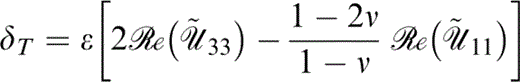
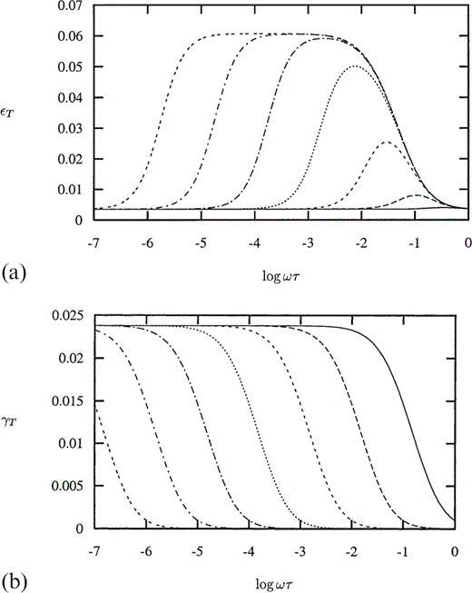
We start by considering the variation of Thomsen's parameters (see Appendix B) with the non‐dimensional frequency Ωτ and the constants P^k and P^m. From the definitions (eqs B1, B2 and B3),

and

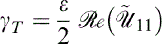
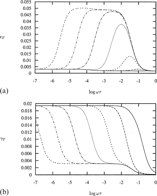
to first order in crack density ε. Thus ε_T (a measure of the P‐wave anisotropy) is independent of P^m and, from Fig. 3(a), is described by a bell‐shaped curve for lower values of P^k that develops a flat top for higher values, while γ_T (a measure of the SH‐wave anisotropy) is independent of P^k and is described by a monotonically decreasing curve (see Fig. 3b); δ_T depends upon both P^k and P^m.

We see from Fig. 3(a) that increasing P^k results in an increase in the magnitude of the peak of ε_T up to a maximum reached at P^k≃10⁶ and a decrease in the value of Ωτ at which the peak occurs, at approximately Ωτ=(P^k)^−1/2—thus we see that the term (Ωτ)²P^k dominates eq. (56). Increasing P^k still further does not change the peak value of ε_T, but broadens the range of Ωτ within which ε_T is non‐negligible.

From Fig. 3(b) it can be seen that an order of magnitude increase in the value of P^m results in an order of magnitude decrease in the value of Ωτ at which a transition is made from the maximum to the minimum values of γ_T (as Ωτ→∞, E_m→0 such that M′→∞ and thus 풰˜₁₁→0) with the transition occurring over a range [0.1 (P^m)⁻¹, 10 (P^m)⁻¹] of Ωτ.

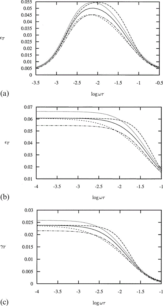
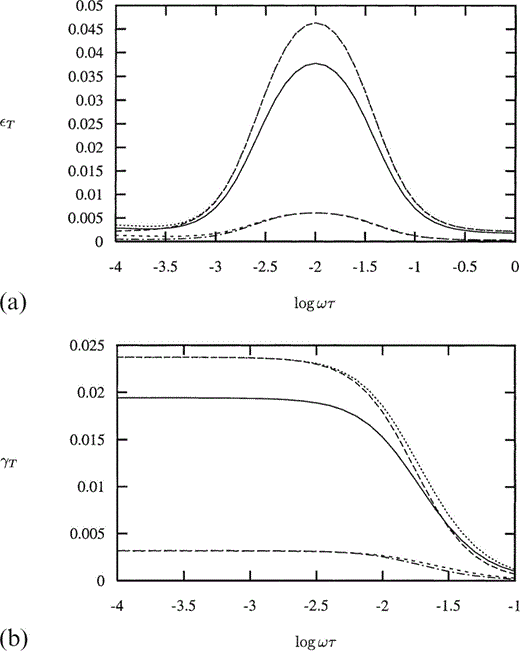
We now consider the effect upon Thomsen's parameters of the distribution parameter δ and the crack density ε. In Fig. 4(a) we consider the effect of δ and ε upon ε_T, for P^k=10⁴. We see that a decrease in the variance of the distribution increases the value of ε_T at its peak—that is, it increases the degree of anisotropy, as we would expect. The greatest value of ε_T is obtained for δ=0, where all the cracks have the same aspect ratio. Although this case corresponds to an anomalous result for the elastic moduli at low frequencies, we see that the behaviour of ε_T in the limit δ→0 is not remarkable. Away from the peak value, little change is seen in the value of ε_T when δ is varied. Furthermore, we note that an increase in the crack density also serves to increase the peak value of ε_T—thus decreasing the variance from 0.703 to 0 (the aligned case) produces a result that is very similar to that achieved by increasing the crack density from 0.2 to 0.0216, and similarly, increasing the variance to 1.0 (an exponential distribution) is seen to be almost equivalent to decreasing the crack density to 0.0182.

So can we distinguish between the effects of the crack density ε and the variance of the aspect ratio distribution δ? At values of Ωτ away from the peak value of ε_T, a change in δ will not affect the value of ε_T, whereas an increase or decrease in ε will cause an increase or decrease, respectively, in ε_T; however, this effect is barely discernible for such small changes in ε as those discussed above. For larger values of P^k, we are more able to distinguish between the two effects (see Fig. 4b), where now P^k=10⁸. Only a small change is seen in ε_T with δ, but a notably different change is seen when adjusting the value of ε.

Fig. 4(c) shows how γ_T varies with δ and ε, for P^m=10². We see that a reduction in the variance of the aspect ratio distribution will increase the value of Ωτ at which the transition from the maximum to minimum values of γ_T begins, without affecting the point at which the minimum value is reached. This effect can be distinguished from changes in the value of ε, which clearly increases or decreases the maximum value of γ_T with Ωτ as it is increased or decreased respectively.

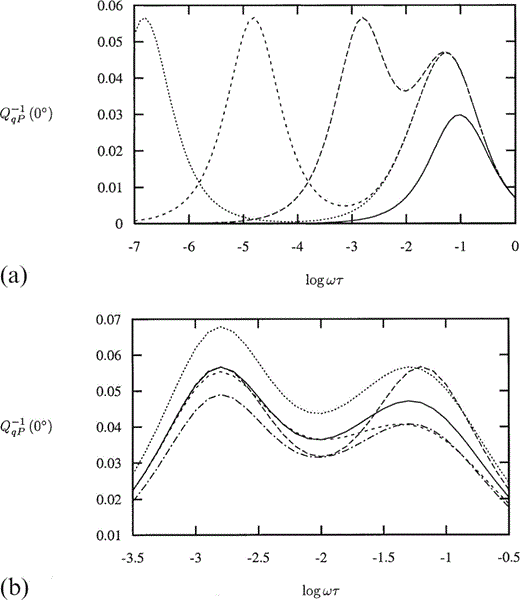
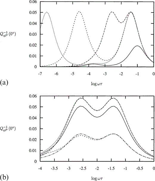
The attenuation coefficients Q⁻¹ for the three waves are defined in eqs (C13), (C14) and (C15); these are dependent upon the incident angle of a wave. For an incident wave parallel to the direction of the crack normals (and thus perpendicular to the cracks), the x₃‐direction, the change in Q⁻¹_qP with frequency is shown in Fig. 5(a) for different values of the parameter P^k and Fig. 5(b) for different values of ε and δ. For values of P^k smaller than about 10³ there is a single peak in the value of Q⁻¹_qP. For sufficiently large P^k this peak remains at a fixed frequency and amplitude, while a second peak occurs at a frequency that decreases as P^k increases. Comparing Figs 3(a) and 5(a), we see that the frequencies at which the peaks in the attenuation parameter Q⁻¹_qP occur coincide with the frequencies of the maximum gradient in the corresponding plot of ε_T. A change in ε clearly changes the magnitude of both peaks (see Fig. 5b) and a change in δ produces a larger change in the magnitude of the higher‐frequency peak than it does in the lower‐frequency peak. Indeed, for larger values of P^k, a change in δ has no effect on the magnitude of the low‐frequency peak. Thus, we can always adjust the value of ε to mimic the effect on the high‐frequency peak in Q⁻¹_qP of a change in δ, but both peaks cannot be simultaneously matched. The relative heights of the two peaks should be able to give us an indication of the value of δ, assuming that both frequencies are seismically possible. At an incident angle parallel to the cracks, Q⁻¹_qP shows a similar variation with the parameters P^k, ε and δ, but is of an order of magnitude smaller (not shown).

Being able to distinguish between the effects of δ and ε on Q⁻¹_qSH is far less likely (see Fig. 6). The frequency at which the peak in Q⁻¹_qSH occurs coincides with the frequency at which the corresponding plot of γ_T has a maximum gradient (see Fig. 3b).

8 VARIABLE ORIENTATION

We shall now consider the effects of allowing the orientation of the crack normals to vary while keeping α constant; thus

We find that

where

and

풰¯₁₁ is given by

8.1Modelling the distribution

We shall make the assumption that the crack distribution is rotationally symmetric—that is, the cracks are uniformly distributed with respect to φ—and consider distributions for n that are concentrated around a mean orientation. We use the Watson distribution (Mardia 1972, Fisher 1987) , a bipolar distribution, such that

where

and we have restricted the range of θ to half that given in the original definition of the distribution, to avoid any ambiguity in the definition of crack‐normal orientation ( as Peacock & Hudson 1990). We shall take θ₀=0 so that the mean orientation of the normal, n⁰=(0, 0, 1)^T, is along the x₃‐axis, and the resulting effective medium is vertically transversely isotropic.

The parameter k is a measure of the variance of the distribution,

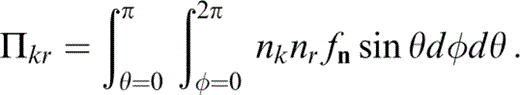
where the integral I_m,n is defined by eq. (D1). k=0 corresponds to a uniform (isotropic) distribution and as k→∞ the distribution approaches a delta‐like function (eq. 51), so that the cracks are fully aligned. With this distribution, we find that {Π_kr} is diagonal, with

To evaluate the components of {Ω_tkrlus} we must find {l_ij}, given that

The rotation {l_ij} is given by Fisher (1987) as

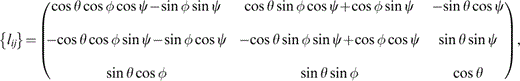
where ψ represents an arbitrary rotation about the x₃‐axis. {T_krus} (eq. 74) is independent of the angle ψ, and those elements of {Ω_tkrlus} that contribute to {T_krus} are given in Appendix D.

8.2 Results

The effect upon Thomsen's parameters of the crack orientation distribution is now considered. We examine how they vary with Ωτ, P^k, P^m, ε and the distribution parameter k. We use the same values of all of the parameters as with the variable aspect ratio model.

We no longer have such simple expressions for Thomsen's parameters as eqs (69), (70) and (71), while γ_T remains independent of the parameter P^k, and ε_T now depends upon both P^k and P^m, as does δ_T, as before. When k=0.0, the distribution of crack‐normal orientations is uniform (i.e. isotropic) and all of Thomsen's parameters are identically zero. For k=10.0, the distribution of crack‐normal orientations about the mean is given in Fig. 7, and with P^m=10⁴, the variation of ε_T with Ωτ for a range of values of P^k is shown in Fig. 8(a). We note that Figs 8(a) and 3(a) look very similar; however, it is not now until P_k=10⁷ that ε_T reaches its largest peak value. The peak values obtained are less than the corresponding ones in Fig. 3(a).

By choosing a different value of P^m, we would have made only a minimal difference to Fig. 8(a). A smaller value of P^m would result in a larger value for ε_T, but only for smaller values of P^k, whereas a larger value of P^m would reduce ε_T for the larger values of P^k—these effects would be difficult to distinguish from either a larger value of the distribution parameter k or a more tightly concentrated distribution or an increased crack density ε.

In Fig. 8(b) we show the variation of γ_T with P^m (independent of P^k); compare this with Fig. 3(b). Certainly there is a considerable similarity, as with ε_T; however, for P^m=10⁴ and higher, the transition from the maximal to minimal values of γ_T occurs over a larger range of Ωτ than for the variable aspect ratio model; indeed, for P^m higher than 10⁴, γ_T appears to reach a non‐zero minimal value before finally approaching zero at higher values of Ωτ.

For the choice of parameters P^k=10⁴ and P^m=10⁴, the effect on ε_T of a change in k is indistinguishable from a change in ε, except perhaps at low frequencies. From Fig. 9(a) it is seen that increasing k to infinity (the fully aligned limit) appears identical to increasing the crack density to ε=0.0242, while decreasing k to 1.0 appears indistinguishable from decreasing ε to 0.0034. Altering the value of P^k or P^m does not increase the difference between the effect on ε_T of changes in k and ε.

For a smaller value of k, the difference between Figs 8(b) and 3(b) is amplified, while for a larger value of k, Fig. 8(b) becomes indistinguishable from Fig. 3(b)—compare the long dashed lines in Figs 4(c) and 9(b). This is as we would expect, that a very small perturbation in either the crack‐normal or aspect ratio distributions from the perfectly aligned identical aspect ratio limit would be indistinguishable.

A change in k is distinguishable from a change in ε, although only at higher frequencies (see Fig. 9b), where at low frequencies increasing k to infinity appears equivalent to increasing ε to 0.242 and decreasing k to 1.0 is almost equivalent to decreasing ε to 0.0034. The P‐wave attenuation coefficient, Q⁻¹_qP, also shows similar behaviour for this model as it does for the variable aspect ratio model (see Fig. 10a). A change in the value of P^m would alter this figure marginally for the smaller values of P^k only.

The change in Q⁻¹_qP with a change in k or ε is illustrated in Fig. 10(b). We note that while we see a close correspondence between increasing k to infinity and increasing ε to 0.023, and also between decreasing k to 1.0 and decreasing ε to 0.01, the values of ε at which this correspondence occurs differ from those at which a similar correspondence occurs in ε_T (see Fig. 9b). As with the variable aspect ratio model, the peak in Q⁻¹_qP is seen to occur at the same frequency at which ε_T has a maximum gradient.

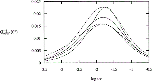
A variation in the SH‐wave attenuation coefficient, Q⁻¹_qSH, is seen with a variation in P^m ( Fig. 11a). It is seen that for large enough values of P^m, there is a second (small) peak in Q⁻¹_qSH perpendicular to the cracks. For P^m=10⁴, such that a second peak occurs, the variation in Q⁻¹_qSH with k and ε is given in Fig. 11(b). While we are able to match the height of the low‐frequency peak resulting from a change in k by a corresponding change in ε, the existence and relative height of the higher‐frequency peak enables us to distinguish between the two competing effects.

For lower values of P^m, at which this second, smaller peak does not occur, the effects of k and ε become indistinguishable. The peaks in Q⁻¹_qSH occur at the frequency at which γ_T has a maximum gradient, thus for smaller P^m when γ_T exhibits only one region of change (see Fig. 8b), there is only the one peak in Q⁻¹_qSH, while for larger P^m, Q⁻¹_qSH exhibits a second peak.

9 DISCUSSION

We have seen that for both the variable aspect ratio and the variable orientation models there exist critical (non‐dimensional) frequencies in both the variation of Thomsen's parameters and the attenuation coefficients at which either a peak is reached or a transition is made from one value to another. The significance of these critical frequencies is their potential use in determining estimates of the unknown parameters within the model—ε, α₀, δ, k and τ;n⁰ can be determined as the direction corresponding to maximum attenuation. We rely, then, on the value of τ being such that the critical (non‐dimensional) frequencies are attainable within the frequency range that can be achieved seismically (1<Ω<10⁴ rad s⁻¹). Estimates of τ(Hudson 1996; O’Connell & Budiansky 1977 lead us to believe that this is possible.

On consideration of either the variable aspect ratio or variable orientation model alone, it appears that we ought to be able to differentiate between the effects of ε and δ in the former, and ε and k in the latter, via Thomsen's parameters and the attenuation coefficients. Our ability to do this depends not only on the range of values of Ωτ at our disposal, but also on the values of P^k and P^m, both of which are inversely proportional to τ.

As might be expected, a very small variance in the aspect ratio distribution is not readily distinguishable from a similarly small variance in the orientation distribution. However, for larger variances, these effects do indeed become more distinguishable.

We could allow both the orientation and the aspect ratio to vary simultaneously, leading to an expression for the first‐order correction to the elastic constants of the same form as eq. (73), but with a more elaborate expression for T_krus. For completeness, this form is given in Appendix E, although it is used nowhere within this paper.

Although the limit of fully aligned cracks of identical aspect ratio is a singular limit, in so far as its behaviour at low frequency is as if isolated, as opposed to undrained for non‐aligned cracks, we see that this limit is not a significant one—there is no singularity in the behaviour of either Thomsen's parameters or the attenuation coefficients in this limit.

10 CONCLUSIONS

The model proposed by Hudson (1996) for the transfer of fluid between connected cracks via non‐compliant pores has been extended to allow for a continuous distribution of values of both crack orientation and aspect ratio. This more realistic model has the expected properties that at high frequencies the cracks behave as if isolated, while at low frequencies they behave as if undrained, and agree with the results of Brown & Korringa (1975). In the fully aligned limit they behave as if isolated at both high and low frequencies.

We looked separately at the cases of allowing the aspect ratio and orientation to vary, while keeping the other fixed, and studying the frequency dependence of Thomsen's parameters and the attenuation coefficients. For both models, we considered whether or not we were able to notice, and differentiate between, the effects of the variance of the distribution and the crack density of the model. Furthermore, we addressed the issue of differentiating between the effects of the variable aspect ratio and orientation.

We believe that it is possible to both notice and differentiate between the effects of the crack density and the variance of one or other of the models. Furthermore, we believe that there is some hope of distinguishing the effects of the variance of one model from those of the other.

Critically, however, there is a dependence upon the undetermined parameter corresponding to the relaxation time of pressure equalization between cracks, τ. Although estimates of this parameter have been made (Hudson 1996; O’Connell & Budiansky 1977), a numerical investigation remains the subject of future work.

Acknowledgments

I would like to thank Stephen J. Hay at Statoil, Norway, for permission to use the crack dimension data from his thesis ( Hay 1988), John A. Hudson at DAMTP, University of Cambridge, for the content of Appendix A, and Enru Liu at the British Geological Survey for support and encouragement. The work was sponsored by the National Environment Research Council through project GST022305 as part of the thematic programme ‘Understanding the micro‐to‐macro behaviour of rock fluid systems (μ2M)’ and is published with the approval of the Director of the British Geological Survey.

References

APPENDIX A:LOCAL DIFFUSION EQUATION

Let ρ_fⁿ, φ_n and p_fⁿ be the fluid density, volume and pressure in the nth crack. The mass flow into the nth crack is

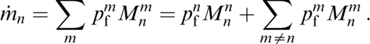
Let p_f^m be the fluid pressure distribution due to unit pressure in the mth crack and zero in the rest. Let M_n^m be the associated flow into the nth crack. Then,

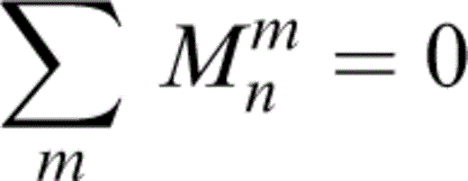
Fluid mass is preserved and does not concentrate in the pores, so

or

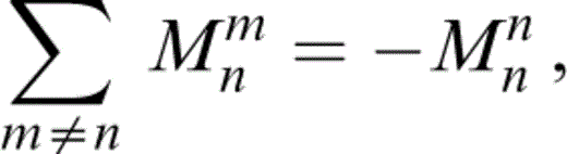
thus

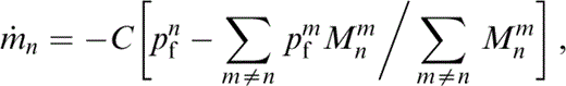
where

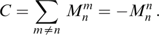
We make the approximation

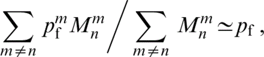
since it is clearly a weighted average of the pressure in the cracks (excluding the nth) and the weights decrease with distance, becoming negligible (probably) at several crack spacing lengths. Then

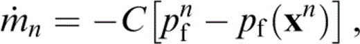
where p_f (xⁿ) is an average of the p_fⁿ over a region 풟_n centred on xⁿ, the centroid of the nth crack. Taking the average over 풟_n,

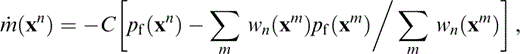
where w_n are weight functions. Thus,

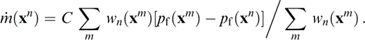
We identify

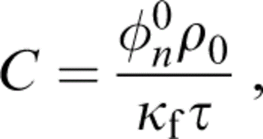
a constant of appropriate dimensions, containing an unknown relaxation parameter, τ.

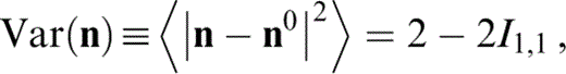
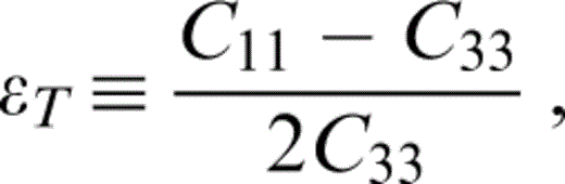
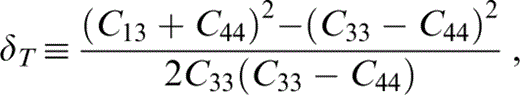
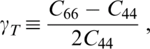
APPENDIX B:THOMSEN’S PARAMETERS

In the conventional condensed, two‐subscript, 6×6 matrix notation, pairs of indices are represented as a single index: ij→p, kl→q, such that 11→1, 22→2, 33→3, 23→4, 13→5 and 12→6. We thus use the representation C_pq, rather than c_ijkl (eq. 1).

We make use of the anisotropy parameters defined by Thomsen (1986) for vertically transversely isotropic material,

where the real part is assumed when the stiffnesses are complex.

We may use the wave speeds, eqs (C9) and (C10), to calculate two of these parameters,

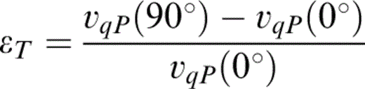
and

to first order in ε.

APPENDIX C:WAVE SPEEDS AND Q

We make the assumption that the mean wave is a plane harmonic wave, u=be^ik . x and substitute this into the time‐harmonic equation of motion,

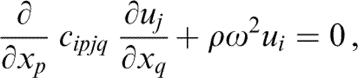
where ρ is the density of the matrix and Ω the frequency of the propagating wave. We have

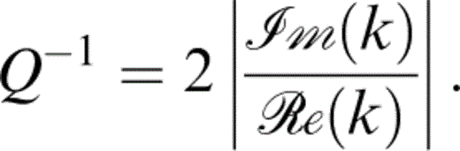
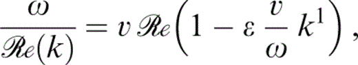
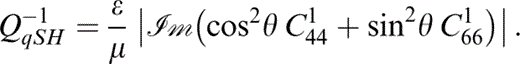
The attenuation coefficient Q⁻¹ is given by

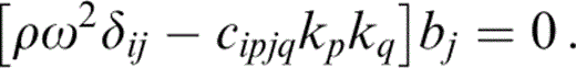
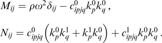
For a given Ω, we let k=k⁰+εk¹ and b=b⁰+εb¹ and equate coefficients of ε⁰ and ε¹ in eq. (C2). Thus, at 풪(ε⁰) and 풪(ε¹) we have

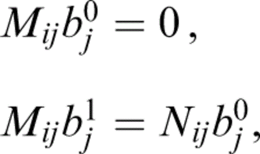
where

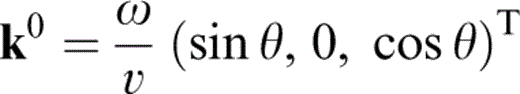
The 풪(ε⁰) term is just the isotropic result. To first order, the cracks have normal (0, 0, 1)^T and the rotational symmetry of the problem ensures that the material is transversely isotropic, so that, for a given Ω, we can rotate the (x₁,x₂) plane such that

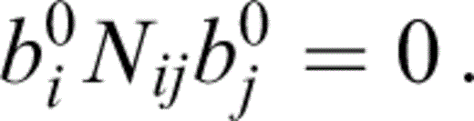
for some incident angle θ, where v=v_P or v_S, corresponding to quasi‐P (qP) waves, or quasi‐S (qS) waves, respectively. For the qP wave, we have b⁰_qP=(sin θ, 0, cos θ)^T, while for the qS waves we have b⁰_qSV=(cos θ, 0, −sin θ)^T or b⁰_qSH=(0, 1, 0)^T, corresponding to qSV and qSH waves, and we are free to choose the magnitude of b⁰. Pre‐multiplication of the 풪(ε¹) term with b⁰ yields a single equation for the components of k¹,

On the assumption that k¹ is parallel to k⁰, this becomes an expression for the magnitude k¹ of k¹.

The wave speeds, to first order, are given by

for v=v_P or v_S, and we take the appropriate values of k¹. Thus, the normalized wave speeds are

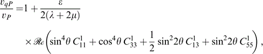
These are equivalent to Hudson (1981).

From eq. (C3), the attenuation coefficient is given by

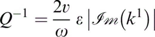
to first order for v=v_P or v_S and the appropriate k¹. Thus,

APPENDIX D:NON‐ZERO CONTRIBUTING TERMS OF Ω

We start by defining the integral

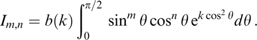
The components of Ω_tkrlus that contribute to T_krus (eq. 74) are

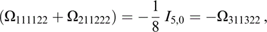
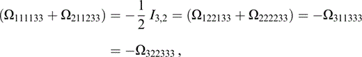
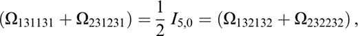
and those related to the above by the symmetries

APPENDIX E:VARIABLE ASPECT RATIO AND ORIENTATION

For completeness, we give an expression for the first‐order correction to the elastic constants derived by allowing both the aspect ratio and the orientation to vary while remaining independent of one another:

where