


Summary
This paper aims to present a new method to calculate surface waves in 3-D sedimentary basin models, based on the direct boundary element method (BEM) with vertical boundaries and normal modes, and to evaluate the excitation of secondary surface waves observed remarkably in basins. Many authors have so far developed numerical techniques to calculate the total 3-D wavefield. However, the calculation of the total wavefield does not match our purpose, because the secondary surface waves excited on the basin boundaries will be contaminated by other undesirable waves. In this paper, we prove that, in principle, it is possible to extract surface waves excited on part of the basin boundaries from the total 3-D wavefield with a formulation that uses the reflection and transmission operators defined in the space domain. In realizing this extraction in the BEM algorithm, we encounter the problem arising from the lateral and vertical truncations of boundary surfaces extending infinitely in the half-space. To compensate the truncations, we first introduce an approximate algorithm using 2.5-D and 1-D wavefields for reference media, where a 2.5-D wavefield means a 3-D wavefield with a 2-D subsurface structure, and we then demonstrate the extraction. Finally, we calculate the secondary surface waves excited on the arc shape (horizontal section) of a vertical basin boundary subject to incident SH and SV plane waves propagating perpendicularly to the chord of the arc. As a result, we find that in the SH-incident case the Love waves are predominantly excited, rather than the Rayleigh waves and that in the SV-wave incident case the Love waves as well as the Rayleigh waves are excited. This suggests that the Love waves are more detectable than the Rayleigh waves in the horizontal components of observed recordings.
1 Introduction
Seismic ground motion inside sedimentary basins is typically characterized by secondary surface waves. These waves prolong the duration of the ground motion with large amplitudes and long periods (several seconds to around 10s). It has been widely recognized that surface waves are excited when seismic waves are incident on strong lateral heterogeneities such as basin edges and the surface wave energy is then trapped inside the basins. The importance of the secondary surface waves has been pointed out in terms of engineering seismology, because enormous damage to buildings in Mexico City during the 1985 Michoacan earthquake is considered to have been caused by long-lasting secondary surface waves with a period of 3s (Kawase & Aki 1989). The long duration of ground motion can be attributed to superposition of secondary surface waves excited in basin edges and laterally multireflected waves from basin boundaries associated with propagation. To understand such complex wavefields physically, it is meaningful as a first step to investigate the excitation of the secondary surface waves. We are particularly interested in finding out on which part of basin boundaries they are excited and how large the secondary Rayleigh and/or Love waves are subject to a given incident wave.
Considerable observational data have been accumulated so far. Kinoshita (1992) found secondary Love waves with a period of 8s in the Kanto basin, Japan. Hatayama (1995) also detected remarkable secondary Love waves with a period of 3s in the Osaka basin, Japan. Both authors analysed small-aperture array recordings and traced the secondary source areas back to the basin edges. Furumura (1994) observed not only secondary Love waves but also Rayleigh waves in the Tokachi basin, Hokkaido, Japan. Numerical techniques are also used to interpret the observed recordings. Yamanaka, Seo & Samamo (1989, 1992) found Love waves with a period range between 5 and 10s in the Kanto basin and concluded from 2-D finite-difference modelling that they were secondarily excited surface waves. These studies, however, do not provide us with a systematic understanding of the excitation of the secondary surface waves. We also note that Love waves are more frequently observed than Rayleigh waves. This is also supported by Toshinawa & Ohmachi (1992) and Kato, Aki & Teng (1993). They showed using 3-D numerical modelling that Love waves with a period of 8s were predominant in the main part of the later arrivals observed in the Kanto basin.
Many articles call for the necessity of 3-D modelling to investigate quantitatively ground motion in basins. For example, Sánchez-Sesma, Pérez-Rocha & Reinoso (1993a) emphasize 3-D effects in interpreting the recordings in Mexico City valley. Hatayama (1995) also suggested the necessity of 3-D modelling, because the large amplitude of the secondary Love waves could not be reproduced by the 2-D indirect boundary element method (BEM) (Sánchez-Sesma, Ramos-Martínez & Campillo 1993b). Many authors have vigorously developed numerical techniques to calculate seismic wavefields in 3-D basin models based on various methods: (1) the finite-difference method (e.g. Yomogida & Etgen 1993; Graves 1996; Pitarka et al. 1997); (2) the BEM (e.g. Sánchez-Sesma & Luzön 1995); (3) the Aki–Larner method (e.g. Horike, Uebayashi & Takeuchi 1990). Most of these techniques aim at calculating the total wavefield and they are useful especially in simulating observed recordings. The calculation of the total wavefield, however, does not match our purpose, because the excited secondary surface waves will be contaminated by the reverberation of amplified body waves and the lateral multireflection of the secondary surface waves.
In order to calculate Love wavefields in 2-D basin models, Fujiwara & Takenaka (1994a) proposed an efficient method based on the direct BEM formulation. This method relies on the assumption that the media inside and outside a basin consist of several flat-layered half-spaces divided by vertical boundaries and follows the boundary integral equations set for each domain using the Green's functions represented by wavenumber integrals. Consequently, the number of boundary elements can be reduced as compared with the BEM using the full-space Green's functions and the BEM using the half-space Green's functions (Kawase 1988), because only the vertical boundaries require discretization. Their method enables us to calculate the surface waves alone by using the Green's functions represented by normal-mode summation and solutions on the vertical boundaries, and this cannot be achieved in the BEM using the full-space Green's functions. Their method, moreover, introduces the propagation operator in the lateral direction and accomplishes a desire not to calculate the total surface waves but to separate them into elementary waves that have the physical concept of phase. This means that we can evaluate excited surface waves alone. Although Hisada, Yamamoto & Tani (1992) proposed a very similar method before Fujiwara & Takenaka (1994a) did, their formulation does not consider such separation. Hisada, Aki & Teng (1993) also extended the method to calculate the surface waves alone in 3-D basin models. Their method, however, deals roughly with the truncation associated with the discretization of boundary surfaces and we shall make a detailed discussion of this point in the later part of our work.
This paper aims at presenting a new method to calculate surface waves excited on parts of the boundaries of 3-D sedimentary basin models, separating them from the total wavefield. Our method is motivated by the basic ideas included in Fujiwara & Takenaka (1994a). For the separation of the total wavefield, however, we are guided by the reflection and transmission operators defined in the space domain (Fujiwara & Takenaka 1994b) instead of the propagation operator, because the former are richer in physical meaning. For a systematic grasp of the excitation of surface waves, plane-wave incidence is appropriate, because horizontal motion of incident waves is polarized in the same direction at every point on a basin boundary. We thus concentrate on plane-wave incident cases in our numerical experiments, although it is straightforward to apply our method to point sources. When we obtain the separated wavefield, comparison will be needed with the total wavefield to prove the validity of our method, thus in Section 2 we begin with the direct BEM formulation to calculate the total wavefield in a whole-basin model. In this case, we encounter problems caused by the truncation of vertical boundary surfaces at a certain depth. To compensate this truncation, we first introduce an approximate algorithm making use of the solutions for 1-D reference media (reference solution approximation). In Section 3 we present an idea to separate the 3-D wavefield into the elementary waves with a formulation that uses the reflection and transmission operators, and we prove that, in principle, it is possible to extract surface waves excited on part of the basin boundaries from the total wavefield. We then realize the above idea in the direct BEM algorithm. Again, we encounter the problem arising from lateral and vertical truncation of boundary surfaces extending infinitely in a half-space. To overcome this problem, we first present a reference solution approximation technique making use of 2.5-D and 1-D solutions, where the 2.5-D wavefield is a 3-D wavefield with 2-D subsurface structures. We finally demonstrate the separation of secondary surface waves excited by plane-wave incidence. In Section 4 we solve the problem of an arc shape (horizontal section) of vertical boundary subject to incident SH and SV plane waves propagating perpendicularly to the chord of the arc, and discuss the excitation of the secondary Rayleigh waves and Love waves.
2 Calculation Of The Wavefield For A Whole Basin
2.1 Description of the method
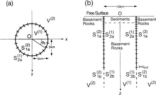
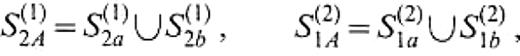
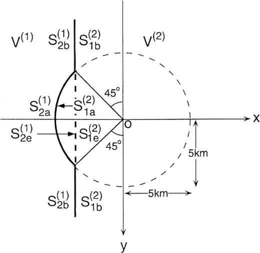
We consider a 3-D model of a sedimentary basin as depicted in Fig.1. It consists of two flat-layered domains represented by V(1) and V(2). Let S(1)=S(1)2a∪S(1)2b be the boundary of the domain V(1) that is in contact with V(2) and S(2)=S(2)1a∪S(2)1b be the boundary of the domain V(2) that is in contact with V(1). The boundaries S(1)2a and S(2)1a are connected to S(1)2b and S(2)1b, respectively, at z=zcut. The boundaries S(1)2b and S(2)1b extend to infinite depth. In the following formulation, we use the Cartesian coordinate system and assume a time dependence of eiωt.
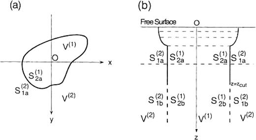
Illustration of a 3-D basin model with a horizontally closed vertical boundary. (a) Plan view; (b) vertical section. The model consists of two flat-layered half-spaces: V(1) and V(2). S(1)2a∪S(1)2b is the boundary of the domain V(1) that is in contact with V(2) and S(2)1a∪S(2)1b is the boundary of the domain V(2) that is in contact with V(1). S(1)2a and S(2)1a are connected with S(1)2b and S(2)1b, respectively, at z=zcut. S(1)2b and S(2)1b extend to infinite depth.
2.1.1 Displacement and traction on S(k)
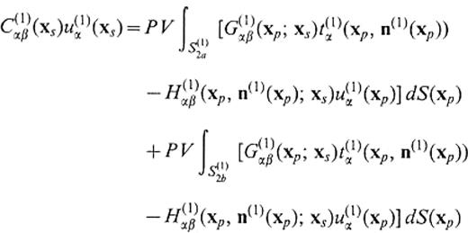
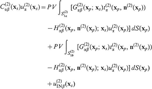
The boundary integral equations are given by
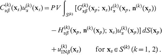
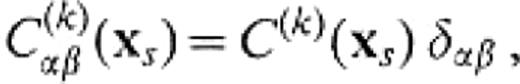
The symbol PV denotes the principal value in Cauchy's sense. The greek subscripts stand for Cartesian components and Einstein's convention is understood. The functions u(k)α(xp)and t(k)α(xp, n(k)(xp)) are the displacement and the traction, respectively, at xp∈S(k), and n(k)(xp) is the unit normal vector pointing out of V(k) at xp. G(k)αβ(xp;xs)is the Green's function for the medium of V(k), that is the displacement in theα -direction at xp for a unit force acting in the β -direction at xs, and H(k)αβ(xp, n(k)(xp);xs)represents the traction corresponding to G(k)αβ(xp;xs). u(k)INβ (xs) is the incident displace-ment at xs emitted from the source existing in V(k). C(k)αβ(xs)is a constant determined by the boundary shape around xs and is given by

where δαβ is equal to 1 if α is identical to β and 0 otherwise. In the case of a smooth boundary shape, C(k)(xs)=1/2 (Kobayashi 1987). In this study, we use the discrete wavenumber technique (Bouchon 1981) and the global matrix approach (Schmidt & Tango 1986) to calculate the Green's functions and the incident wavefield for the flat-layered media and the half-spaces.
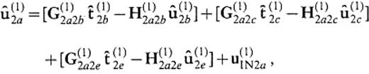
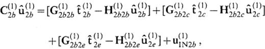
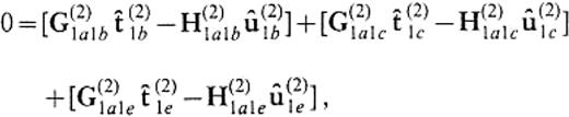
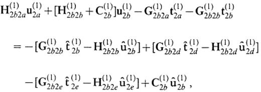
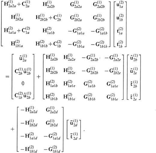
Letting a source exist in V(2), we rewrite eq.(1) in the following operator equations:
and

for {xs∈S(2)1a. The definitions of the operators are described in Appendix A. When oblique incidence of plane wave is considered, we assume a source in V(2) at an infinite distance. Eqs (3) and (4) contain integrals over infinite surfaces in the second brackets of their right-hand sides. We do not treat the displacement and the traction on S(1)2b and S(2)1b as unknown values and replace the infinite integrals by known integral values approximately. This approximation technique was proposed to eliminate non-physical waves caused by truncation of lateral boundaries in the BEM with the full-space Green's functions (Fujiwara & Takenaka 1993; Yokoi & Takenaka 1995; Fujiwara 1996a) and it is known as the ‘reference solution’ approximation. In this study, we first apply the reference solution approximation to the truncation of vertical boundaries. We use the following equations for the approximation:

and
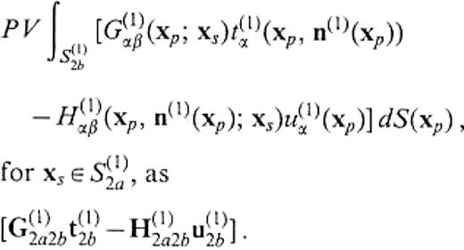
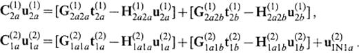
where bbaru(1)2a, bbaru(1)2b, bbart(1)2a and bbart(1)2b denote the solutions for the flat-layered half-space that consists of the same medium as V(1), while bbaru(2)1a, bbaru(2)1b, bbart(2)1a and bbart(2)1b denote the counterparts for V(2). These are the ‘reference solutions’. Subtracting eq.(5) from eq.(3), we have

In the above equation, we can assume that
by choosing an appropriate z=zcut. This assumption relies on the fact that |G(1)2a2b| and |H(1)2a2b| are smaller than |G(1)2a2a| and |H(1)2a2a|, respectively, because of geometrical spreading and the expectation that the true wavefield will be close to the wavefield for the reference media in the depths away from the irregularity localized beneath the surface. Then it follows that

In a similar way, we have

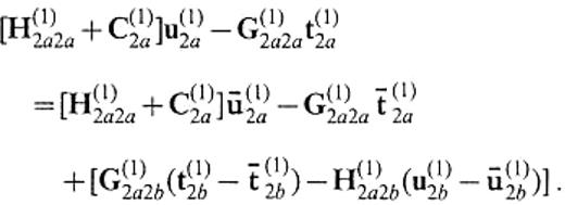
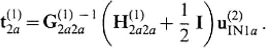
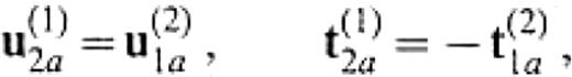
from eqs (4) and (6). Considering the boundary conditions
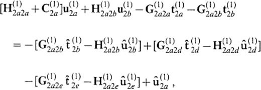
we finally obtain a system to determine u(1)2a and t(1)2a,
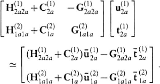
Even if we assume a source in V(1), we have the same equation. We here emphasize that the amount of numerical work to compute the Green's functions is never increased, because the right-hand side has the same operators as those appearing in the left-hand side and these operators are required even if we do not employ the reference solution approximation. If the medium of V(1) is identical to that of V(2), the solution of eq.(13) is the incident wavefield itself, i.e.
We here used the relation C(1)2a+C(2)1a=I, where I is the identity operator.
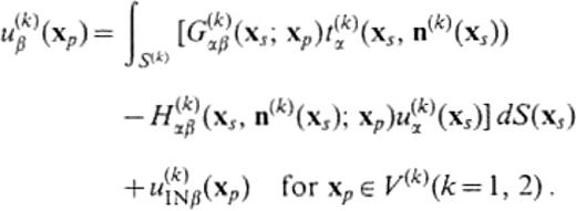
2.1.2 Displacement in V(k)
The displacement u(k)β(x)in V(k) is expressed using the displacement and the traction on the boundary as
We rewrite this equation in the operator form as
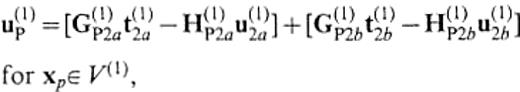
for xp∈V(1), and

for {xp∈V(2). The subscript P indicates the observation points xp. Eqs (17) and (18) also contain integrals over infinite surfaces, so we make use of the reference solution approximation similar to eq.(8) for these integrals. Then we have

and

where bbaru(1)P and bbaru(2)P denote the 1-D solutions at xp for the flat-layered half-spaces that consist of the same media as V(1) and V(2), respectively. If we consider surface waves only, we neglect the integrals over the infinite surface in eqs (17) and (18) and use the surface-wave part in the Green's functions according to Hisada (1993) and Fujiwara & Takenaka (1994a). The displacement of surface waves in V(k) is given by
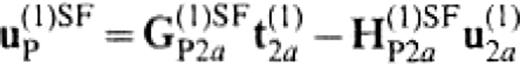
and

G(k)SF and H(k)SF denote integral operators with kernels of the Green's functions calculated by summation of normal modes of Rayleigh waves and/or Love waves. u(2)SFINP1 is the displacement of incident Rayleigh and/or Love wave.
We use constant-value elements to discretize eq.(13) and eqs (19)–(22). This enables us to interpret the above operator equations as matrix forms.
2.2 Numerical results
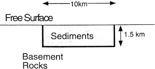
In this paper we use the model of a sedimentary basin depicted in Fig.2 for numerical calculations. The basin forms a disc with a radius of 5km and a thickness of 1.5km. The sediments inside the basin and the basement rocks outside the basin consist of two uniform media with Vp=2.4kms− 1, Vs=0.8kms− 1 and ρ=1.8gcm− 3, and Vp=4.3kms− 1, Vs=2.5kms− 1 and ρ=2.5gcm− 3, respectively. Our calculations are made in a frequency range between 0 and 0.5Hz. We use rectangular boundary elements in the discretization. Horizontally the boundary is divided into 24 elements of equal length, while 18 elements are distributed at unequal intervals in the vertical direction. The first four elements from the free surface have a vertical length of 0.5km and the length increases with depth below the fourth element. This avoids a rapid change in size of elements at the interface between the sedimentary layer and the basement rock. The length of the deepest element is about 1.4km and zcut in Fig.2 is about 15.8km. We determined the value of zcut so large that the fundamental mode of the Love waves over 0.12Hz converges for the layered media inside the basin model. We have 432 elements on the boundary on which the unknown displacement and traction are attributed and consequently the size of the coefficient matrix on the left-hand side of eq.(13) is 2592 × 2592.
A circular disc basin model considered for numerical calculation. The elastic properties of the sediments are as follows: Vp (P-wave velocity)=2. 4kms− 1, Vs (S-wave velocity)=0.8kms− 1 and ρ (density)=1
2.2.1 Necessity of the reference solution approximation
If we do not employ the reference solution approximation, the following system should be solved instead of eq.(13):

Let us consider the case in which the medium of V(1) is identical to that of V(2). Then eq.(23) leads to
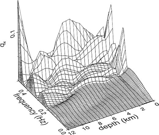
To indicate to what accuracy the traction can be reproduced by the BEM algorithm, we define the following function for a given vertical set of boundary elements:
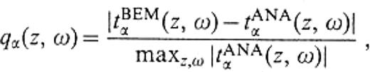
where α denotes Cartesian components. tBEMα(z, ω) and tANAα(z, ω) mean the traction obtained by the BEM algorithm and the analytic traction, respectively. Fig.3 shows qx(z, ω) given by the results from eq.(25) for the vertical set of elements located within the range 45°≤ϕ0≤ 60° , where ϕ0 is an angle with respect to the x-axis. The incident wave is a plane SH wave propagating in the positive direction of the x-axis with an incident angle of 30° with respect to the z-axis. We find that the simple truncation cannot reproduce the correct traction at frequencies above 0.2Hz at all. It is likely that such errors are intuitively attributed to the large size of the boundary elements. However, we also find that these errors are caused by the truncation of boundary elements without the reference solution approximation from the following numerical experiment. As shown in eq.(15), it does not make numerical sense to apply the BEM algorithm with our reference solution approximation to the perfect half-space considered now. Thus let us assume the new model depicted in Fig.4. In this model, a circular boundary surface with a radius of 5km is mathematically added to the model of Fig.2 at z=zcut. We represent this new boundary by S(1)2B, which is the surface of V(1) that is in contact with V(2). Using the known displacement bbaru(1)2B and traction bbart(1)2B on S(1)2B for the perfect half-space, t(1)2a is given by
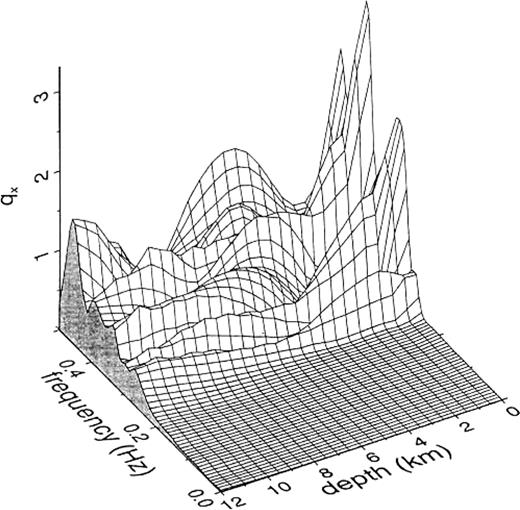
qx(z, ω) (eq.26) given by the BEM with simple truncation for the model in Fig.2, assuming the medium V(1) to be the same as V(2). The incidence is the plane SH wave propagating to the positive direction of the x-axis with an incident angle of 3 0° with respect to the z-axis. The results are shown for the vertical set of elements located within the range 45°≤ϕ0≤ 60° , where ϕ0 is an angle with respect to the x-axis (cf. Fig.1).
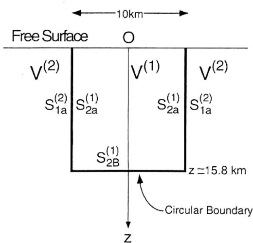
Vertical section of a 3-D circular disc basin model showing the necessity of compensation for the truncation of vertical boundaries. S(1)2B is a circular boundary surface with a radius of 5km added to the model in Fig.2 at z=zcut. The medium of V(1) is assumed to be the same as that of V(2) and as a consequence the model becomes a half-space of the basement rock.
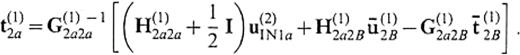
Fig5 shows qx(z, ω) given by the results from eq.(27) for the same vertical set of elements with the same incident wave as in Fig.3. We find that the correct traction can be reproduced by considering the closed boundary surface. The above discussion calls for the necessity of a certain compensation for the truncation of boundary elements, such as the reference solution approximation presented in this study.
qAz, ro) (cq. 26) for the model in Fig. 4 in the case of the same vertica l set of elements and the same incidence as in Fig. 3. Using eq. (27), the BEM solutions are compensated by the displacement and the traction on .si~-
2.2.2 Validity of the reference solution approximation
To prove the validity of our reference solution approxi-mation presented for the truncation of vertical boundaries, we compare our results with those of another method. Fig.6 shows the equivalent model to our disc model. For the comparison, we use the solutions obtained for this model by the BEM with the full-space Green's functions (Fujiwara, personal communication, 1997). In his method, the boundary is divided into triangular elements and the reference solution approximation is taken into account for the truncation of the free surface (Fujiwara 1996a). To compare the full wavefield, we use eq.(19) for our disc model in Fig.2. Fig.7 shows the y-components of responses at free-surface points located inside the basin along the x-axis subject to incidence of the plane SH wave propagating towards the positive direction of the x-axis with an incident angle of 30° . For this incidence, other components vanish along the x-axis due to the symmetry of the model. Our method used about 145 min of CPU time on a Sun Sparcstation with a single 170MHz processor to solve eq.(13) for a single frequency. We find that the results of our method agree very well with the results of the BEM with the full-space Green's functions at most of the frequencies considered, although the discrepancy is not negligible above 0.4Hz. This proves the validity of the reference solution approximation for the truncation of vertical boundaries presented in this study.

Comparison of the y-components of responses at four free-surface points inside the basin along the x-axis. The incidence is the plane SH wave propagating to the positive direction of the x-axis with an incident angle of 30° . The solid lines show the results for the model in Fig.6 by using the BEM with the full-space Green's functions and the broken lines show the results for the model in Fig.2 by using our BEM with the reference solution approximation presented in eq.(13).
2.2.3 Total surface wavefield
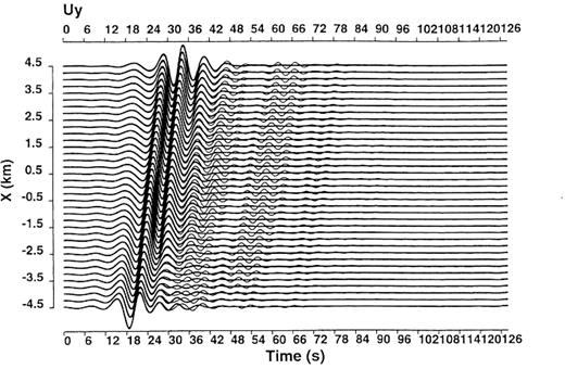
Using eq.(21), we calculated the total Love wavefield excited by the same incident field as before for the sedimentary basin model depicted in Fig.2. Fig.8 shows the y-components of the displacement waveforms convolved with a Ricker wavelet having a centre frequency of 0.12Hz at free-surface points spaced along the x-axis at intervals of 0.25km. In the next section, we describe a method to extract the secondary surface waves merely excited by incident waves from the total surface waves.
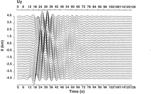
Total Love wavefield at the surface points along the x-axis for the model in Fig.2 subject to the incident plane SH wave propagating to the positive direction of the x-axis with an incident angle of 30° . This wavefield is calculated by using eq.( 21). The surface points are spaced at equal intervals of 0.25km within the range − 4.5 ≤x≤ 4.5km. The displacement time histories are convolved with a Ricker wavelet with a centre frequency of 0.12Hz.
3 Separation Of The Total Wavefield Into Elementary Waves
3.1 Principle
First, we introduce the concept of reflection and transmission operators. This concept was first presented by Fujiwara & Takenaka (1994b) as the counterpart in the space domain for the reflection and transmission matrix in the wavenumber domain defined by Kennett (1983). We then describe how the total wavefield inside a 3-D basin can be separated into elementary waves that have the physical concept of phase.
3.1.1 Reflection and transmission operators
Reflection and transmission across a single vertical interface. We consider a 3-D medium that consists of two domains, V(k) and V(k+ 1). Let S(k)k+ 1 be the infinite boundary of V(k) that is in contact with V(k+ 1), and S(k+ 1)k be the infinite boundary of V(k+ 1) that is in contact with V(k). We define the reflection operator R(k+ 1k) and the transmission operator T(k+ 1k) via the displacement u(k+ 1)k(u(k)INk+ 1) on S(k+ 1)k for the incident displacement u(k)INk+ 1 emitted from the source existing in V(k) as follows (cf. Fig.9a):
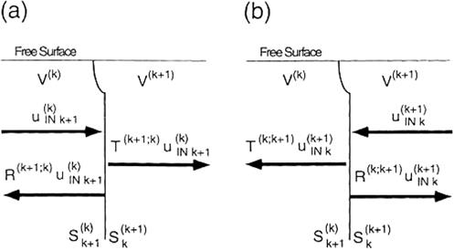
Images of the reflection and the transmission operators. (a) The case where the source exists in V(k); (b) the case where the source exists in V(k+ 1). The notations for the domains and the boundaries are the same as in Fig.1.
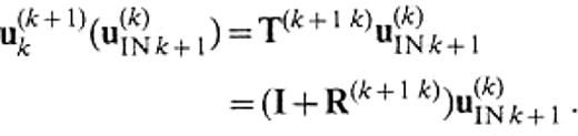
Similarly, we define the reflection operator R(kk+ 1) and the transmission operator T(kk+ 1) via the displacement u(k+ 1)k(u(k+ 1)INk) on S(k+ 1)k as follows (cf. Fig.9b):
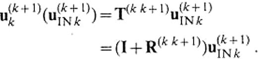
The displacement and the traction on the boundary satisfy the following systems:
where t(k+ 1)k(u(k)INk+ 1) and t(k+ 1)k(u(k+ 1)INk) denote the traction on S(k+ 1)k associated with u(k+ 1)k(u(k)INk+ 1) and u(k+ 1)k(u(k+ 1)INk), respectively. Comparing the solution of this equation with eqs (28) and (29), we have explicit forms of the transmission operators:


where


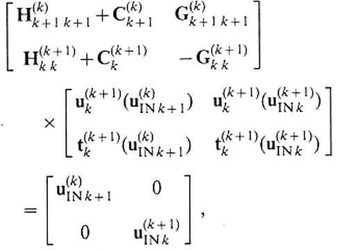
The traction on the boundary is given by
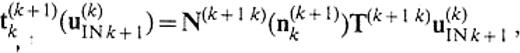

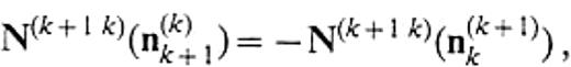
The physical insight into eqs (35) and (36) motivates us to call N(k+ 1k)(n(k+ 1)k) and N(kk+ 1)(n(k+ 1)k) the traction operators, because they play a role of converting the displacement on the boundary to the traction along the unit normal n(k+ 1)k. We can also define the traction operators N(k+ 1k)(n(k)k+ 1) and N(kk+ 1)(n(k)k+ 1) to convert the displacement on the boundary to the traction along the unit normal n(k)k+ 1. The boundary conditions for the traction result in

The boundary traction along n(k)k+ 1 is given by


Representation of phase income. We consider a 3-D medium that consists of three domains, V(k− 1), V(k) and V(k+ 1), as depicted in Fig.10 and let S(k)I be an infinite surface in V(k). Assuming that the medium of V(k+ 1) is identical to that of V(k) and that the source exists only in V(k− 1), the displacement u(k)I(u(k− 1)INk) on S(k)I is expressed by
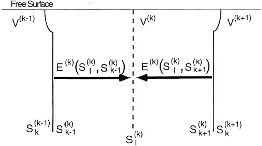
Images of the phase income operator. The notations for the domains and the boundaries are the same as in Fig.1

On the other hand, assuming that the medium of V(k− 1) is identical to that of V(k) and that the source exists only in V(k+ 1), the displacement u(k)I(u(k+ 1)INk) on S(k)I is expressed by

Using eqs (28) and (35) for eq.(41) and using eqs (29) and (40) for eq.(42), the above equations can be rewritten as


where


We call E(k)(S(k)I, S(k)k− 1) and E(k)(S(k)I, S(k)k+ 1)the phase income operators, because they play the role of propagating the incident wave. When the surface waves are considered, we modify these operators into


where G(k)SF and H(k)SF denote the integral operators with kernels of the Green's functions calculated by summation of normal modes of Rayleigh waves (SF=RL) and/or Love waves (SF=LV).
3.1.2 Elementary waves
Let us consider a 3-D medium that consists of three flat-layered domains, V(1) to V(3), as depicted in Fig.11. The boundaries between the domains have semi-infinite extent. We now take the x′-axis and the y′-axis to be normal and parallel, respectively, to the flat part of the boundaries with the same origin as the coordinate (x, y, z). We can prove that this medium is equivalent to a whole 3-D basin model if the medium of V(3) is identical to that of V(1) and if Hto 0, where H is the distance between the flat parts of S(2)1 and S(2)3. Thus we can apply the following discussion for this model to our 3-D basin model.
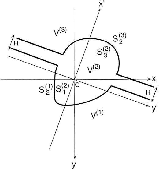
Plan view of the 3-D basin model showing a way of separating the total wavefield into elementary waves. The model consists of three flat-layered half-spaces, V(1), V(2) and V(3). Every boundary surface has a semi-infinite extent. The notations for the boundaries have the same meanings as Fig.1. The x′-axis and they′-axis are normal and parallel, respectively, to the flat part of the boundaries with the same origin as the coordinate (x, y, z).
Let u(2)1 + and u(2)1 − be the waves on S(2)1 propagating in V(2) away from the boundary and close to the boundary, respectively, and let u(2)3 − be the wave on S(2)3 propagating in V(2) away from the boundary. This relies on the fact that the total wavefield can be expressed by a sum of the wave with positive kx′ and that with negative kx′, where kx′ is the x′-component of wavenumber vectors. Assuming the source to be only in V(1), the following equations can be set up:
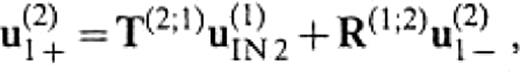

Substituting eq.(50) into eq.(49), we have

By definition, u(2)3 − is expressed by
We can express the displacement u(2)P at a point P in V(2) by
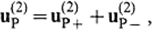
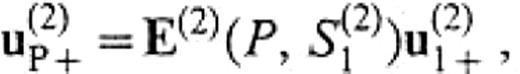
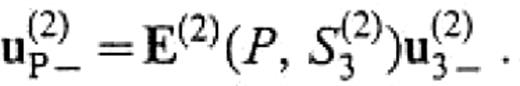
where u(2)P+ and u(2)P− denote the wave with positive kx′ and negative kx′, respectively. By definition, u(2)P+ and u(2)P− are given by
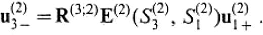
Using eqs (51) and (52) in the above expression, we finally obtain
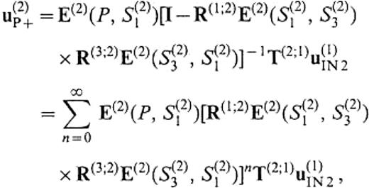
These formulae show that the total wavefield can be expanded into an infinite series in terms of phenomena associated with wave propagation such as reflection and transmission that occur at vertical interfaces. We call each term the elementary wave. For example, E(2)LV(P, S(2)1)T(2;1)u(1)IN2 means the Love wave excited on the boundary between V(1) and V(2) by the incident wave from V(1) and E(2)RL(P,S(2)3)R(3;2)E(2)LV(S(2)3,S(2)1)T(2;1)u(1)IN2 means the Rayleigh wave reflected on the boundary between V(2) and V(3) by the incidence of the Love wave mentioned above. In this study, we calculate E(2)LV(P, S(2)1)T(2;1)u(1)IN2 and E(2)RL(P, S(2)1)T(2;1)u(1)IN2 and examine excitation of the secondary Love and Rayleigh waves subject to plane-wave incidence.
3.2 Realization in the BEM algorithm
In this section, we first present a method to realize in a3-D BEM algorithm the calculation of T(2;1)u(1)IN2 and N(2;1)(n(2)1)T(2;1)u(1)IN2 required to examine the excitation of the secondary surface waves. N(2;1)(n(2)1) appears in the phase income operator E(2)SF(P, S(2)1) expressed by eq.(47). We still consider the model shown in Fig.11. From eqs (28) and (30), we find that the calculation of T(2;1)u(1)IN2 and N(2;1)(n(2)1)T(2;1)u(1)IN2 is simply the solution of the following equation:
The integral operators in the above equation are defined on the infinite surface. We then truncate the boundary surface where the unknown displacement and traction are solved and use the reference solution approximation to compensate for the truncation.
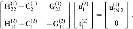
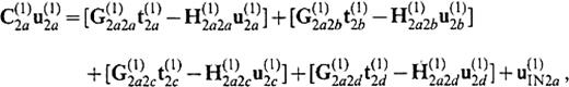
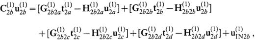
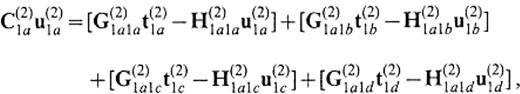
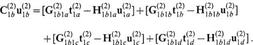
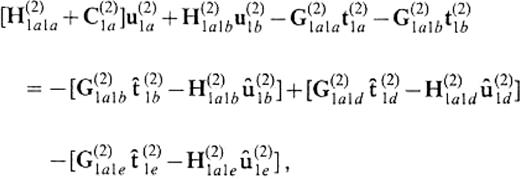
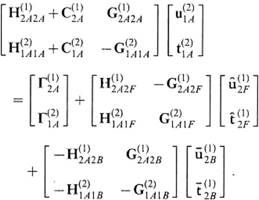
We consider a medium that consists of two flat-layeredhalf-spaces, V(1) and V(2), as shown in Fig.12. Let S(1)2a∪S(1)2b∪S(1)2c∪S(1)2d be the semi-infinite boundary of V(1) that is in contact with V(2) and let S(2)1a∪S(2)1b∪S(2)1c∪S(2)1d be thesemi-infinite boundary of V(2) that is in contact with V(1). S(1)2a and S(2)1a are curved boundary surfaces of part of the basin. S(1)2d is a horizontal lid at z=zcut to connect S(1)2a with S(1)2e and S(2)1d is also a horizontal lid at z=zcut to connect S(2)1a with S(2)1e. S(1)2d and S(2)1d are the mathematical boundaries beyond which there is no change in elastic properties. The surfaces S(1)2b∪S(1)2c∪S(1)2e and S(2)1b∪S(2)1c∪S(2)1e form a vertical and semi-infinite plane. We solve the unknown displacement and traction on S(2)1a∪S(2)1b. Using the operator forms, the boundary integral equations are given by
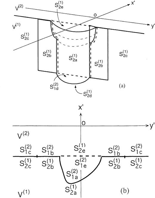
Plan view of a model showing how to extract the secondary surface waves excited on part of a boundary of a 3-D basin model: (a) sketch; (b) plan view. S(1)2a∪S(1)2b∪S(1)2c∪S(1)2d is the semi-infinite boundary of V(1) that is in contact with V(2) and S(2)1a∪S(2)1b∪S(2)1c∪S(2)1d is the semi-infinite boundary of V(2) that is in contact with V(1). S(1)2a and S(2)1a are curved boundary surfaces of part of the basin. S(1)2d is a horizontal lid at z=zcut to connect S(1)2a with S(1)2e and S(2)1d is also a horizontal lid at z=zcut to connect S(2)1a with S(2)1e. S(1)2d and S(2)1d are the mathematical boundaries beyond which there is no change in elastic properties. The surfaces S(1)2b∪S(1)2c∪S(1)2e and S(2)1b∪S(2)1c∪S(2)1e form a vertical and semi-infinite plane. The x′-axis and the y′-axis are normal and parallel, respectively, to the flat parts of the boundaries
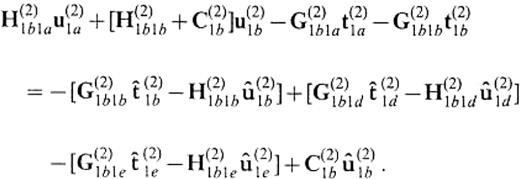
We here rely on the approximation that the displacement and the traction on S(1)2c, S(1)2d, S(2)1c and S(2)1d can be replaced by the solution for the medium without the irregular part surrounded by S(1)2a∪S(1)2d∪S(1)2e, that is the medium that consists of two flat-layered half-spaces bounded by the vertical and semi-infinite plane. This provides us generally with the 2.5-D problem (the problem of the 3-D wavefield in the 2-D subsurface structure). For incident plane waves propagating ∥ to the x′-axis in particular, the solutions are given by the 2-D problem. We represent the 2.5-D solutions by symbols with a hat. The 2.5-D solutions satisfy the following equations:

Using eqs (63)–(66), we can replace the integrals over the infinite surfaces in the third brackets of the right-hand sides of eqs (59)–(62) by the integrals over the finite surfaces; we obtain the following equations by transposition:
In solving the 2.5-D problem, we encounter the truncation problem of the vertical boundary again. Let us truncate the boundary at z=zcut. Then we can follow formally the same formulation to obtain eq.(13), although the kernel of the integral operators should now be replaced by the Green's function for the 2.5-D or 2-D problem. Also, in calculating bcircu(1)2a we can use formally the same equation as eq.(19) but with the kernels for the 2.5-D or 2-D problem. The formulation of eqs (13) and (19) relies on the approximation that the displacement and the traction on the boundary at z≥zcut can be replaced by the 1-D solutions. Thus, we can replace the displacement and the traction on S(1)2d and S(2)1d in eqs (67)–(70) by the 1-D solutions for the flat-layered half-space that consists of the medium of V(1). Representing the 1-D solutions by symbols with a as̄ in Section 2 and considering the boundary conditions
we have the following system:
We redefine the boundary notations as follows:
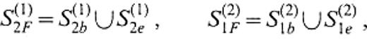

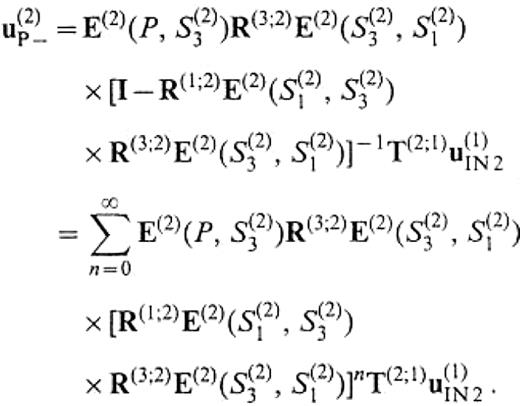
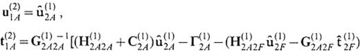
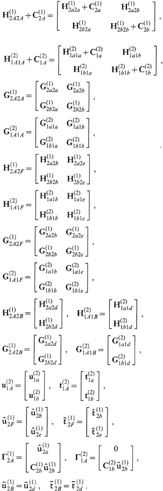
In accordance with this redefinition, we finally obtain the system to give the displacement and traction on S(2)1A as
We describe the definition of the operators appearing in the above equation in Appendix B. If the medium of V(2) is identical to that of V(1), this equation leads to
3.3 Demonstration of extraction
Let us divide the disc basin model in Fig.2 by a vertical cross-section along the y-axis and consider the half-disc model in the domain x≤ 0 as depicted in Fig.13. We discretize the boundary S(1)2a and S(2)1a in the same manner as we adopted for the disc basin model, so we have 12 elements in the horizontal direction. We have eight horizontal elements with an equal length on S(1)2e and S(2)1e, and four horizontal elements with the same length on every side of S(1)2b and S(2)1b. In the vertical direction on every vertical boundary, we have 18 elements by discretizing in the same manner as the disc basin model with zcut≃ 15.8km.

We start by insisting on the necessity of the reference solution approximation presented for the 3-D problem. If we set a pair of boundary integral equations for S(1)2a and S(2)1a without the reference solution approximation and consider the case in which the medium of V(2) is identical to that of V(1), the traction on S(2)1a is given by
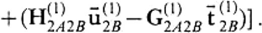
We shall use eq.(26) here again. Figs14(a) and (b) show qx(z, ω) given by the results from eqs (82) and (83), respectively, for the vertical set of boundary elements located within a range 135°≤ϕ0≤ 150° . The incident wave is the plane SH wave propagating to the positive direction of the x-axis with an incident angle of 30° . We find that our reference solution approximation obviously makes the BEM solutions more consistent with the analytic solutions. We also find that the accuracy of the BEM solutions is not so high on the vertical set of elements located in the tip that contacts S(2)1b.
qx(z, ω) (eq. 26) for the model in Fig.13 subject to plane SH-wave incidence propagating in the positive direction of the x-axis with an incident angle of 30° . (a) The results given by the BEM with simple truncation (eq. 83); (b)b the results given by the BEM compensating for truncation of boundaries (eq.82). The results are shown for the vertical set of elements located within the range 135°≤ϕ0≤ 150° .
We next recover the medium of V(2) and calculate E(2)LV(P, S(2)1)T(2;1)u(1)IN2 subject to the same incidence as used for the total Love wavefield shown in Fig.8. In this calcu-lation, we neglect the displacement and the traction on S(2)1b and S(2)1c and take into account the solutions on S(2)1a alone. The thick traces in Fig.15 show E(2)LV(P, S(2)1a)T(2;1)u(1)IN2. For comparison, we extract the Love waves with positive kx, where kx is the x-component of the wavenumber vectors, from the total Love wavefield by using the displacement and the traction only on S(2)1a solved by eq.(13). They are naturally affected by the opposite boundary located in x≥ 0. We show these Love waves by the thin traces in Fig.15. We find clearly that E(2)LV(P, S(2)1a)T(2;1)u(1)IN2 represents the Love waves excited on the boundary S(2)1a and that our BEM algorithm expressed by eq.(80) enables us to evaluate quantitatively the excitation of secondary surface waves caused directly by incident waves and occurring on part of the basin boundaries. This also means that we have made it possible to obtain approximately the solutions that satisfy local boundary conditions on a boundary surface localized in the 3-D space.
Demonstration of the extraction of the Love waves excited on part of a basin boundary from the total Love wavefield
4 Excitation Of Secondary Surface Waves
Using our BEM algorithm presented above, we evaluate the conversion from plane body waves to secondary Love and Rayleigh waves in terms of the horizontal polarization of incident waves. Fig.16 shows a quarter of the boundary of our disc basin model. The basin boundary is considered in the range 135°≤ϕ0≤ 225° , where ϕ0 is an angle with respect to the x-axis. We discretize the boundary S(1)2a and S(2)1a into 12 elements in the horizontal direction. We have 11 horizontal elements with an equal length on S(1)2e and S(2)1e, and four horizontal elements with the same length on every side of S(1)2b and S(2)1b. In the vertical direction on every vertical boundary, we have 18 elements by discretizing in the same manner as the disc basin model with zcut≃ 15.8km. We have 360 elements on the boundary on which the unknown displacement and traction are attributed and consequently the size of the coefficient matrix on the left-hand side of eq.(80) is 2160 × 2160. For this model, we calculate the boundary displacement and traction by T(2;1)u(1)IN2 subject to two types of body-wave incidence: SH wave and SV wave propagating in the positive direction of the x-axis. We then synthesize the displacement of the Love and the Rayleigh wave separately at three surface points close to the boundary (the close points): (x, y)=(− 3.5,0), (− 3.5,1) and (− 3.5,2) in km, and at three surface points away from the boundary (the distant points): (x, y)=(3.5,0), (3.5,1) and (3.5,2).
Our method consumed about 159min of CPU time on the same workstation platform as in Section 2.2.2 to solve eq.(80) for a single frequency. Figs17 and 18 show the Fourier spectra of converted Love and Rayleigh waves at the distant points in the case of SH- and SV-wave incidence, respectively. The incident angle is 30° . We note that the Rayleigh waves are excited even by the SH-wave incidence and that the Love waves are excited even by the SV-wave incidence. If the boundary were a flat surface along the y-direction, these surface waves would never be excited. The curvature of the boundary is responsible for such phenomena as the 3-D effects. The horizontal components of the Rayleigh waves have the first amplitude peak around 0.2Hz at every point in both incidence cases. The horizontal components of the Love waves have an almost flat spectral shape in the SH-wave-incidence case. We thus discuss the time-domain waveforms convolved with a Ricker wavelet with a centre frequency of 0.2Hz and concentrate on the horizontal components in terms of the comparison between Love waves and Rayleigh waves.
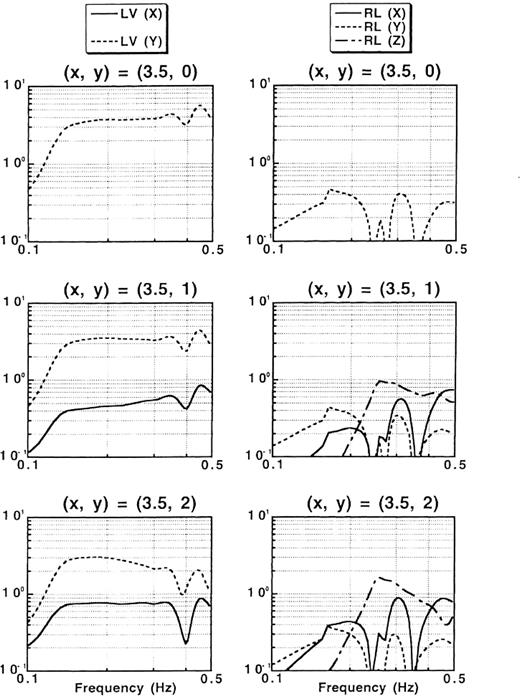
Fourier spectra of converted Love (left) and Rayleigh (right) waves at three surface points subject to SH-wave incidence propagating in the positive direction of the x-axis for the model in Fig.16. The incident angle is 30° . The location of the surface points is as follows: (x, y)=(3.5, 0), (3.5, 1), and (3.5, 2)km.
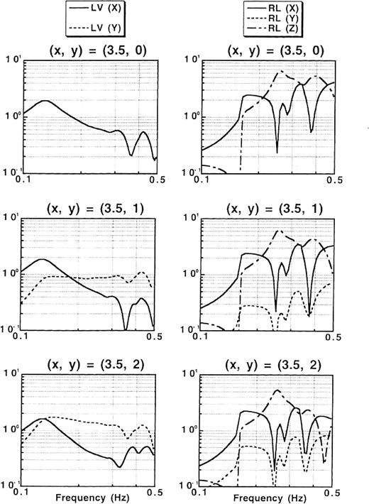
The same as Fig.17, but subject to SV-wave incidence.
Figs19 and 20 show the displacement waveforms of the Love and the Rayleigh waves subject to SH-wave incidence at the close points and the distant points, respectively. These surface waves are constructed by integral contributions of the secondary sources distributed on the boundary. Moreover, in the near field of the source, the Love waves and Rayleigh waves emitted from each secondary source have amplitudes in the radial component and in the transverse component, respectively (Aki & Richards 1980). Thus, rectilinearity of horizontal particle motion is not necessary. In the case ofSH-wave incidence, the horizontal ground motion is overwhelmingly dominated by the Love waves appearing in they-component that corresponds to the horizontal polarization direction of the incident wave. On the other hand, the excitation of the Rayleigh waves is trivial compared with the Love waves both at the close points and at the distant points. Figs21 and 22 are the same as Figs 19 and 20, respectively, but subject to SV-wave incidence. In the case of SV-wave incidence, the Rayleigh waves are more excited than inthe SH-wave-incidence case. At the close points, however, the excitation of the Love waves is comparable to or larger than that of the Rayleigh waves (Fig.21). At the distant points, the Rayleigh waves and the Love waves are predominant in the x- and y-components, respectively, and the Love waves have comparable amplitudes to those of the Rayleigh waves (Fig.22). We obtain the same results in the case of a Ricker wavelet with a centre frequency of 0.3Hz. We also consider an almost vertical incidence with an incident angle of 1° . In this case, only the Love waves excited by the SH-wave incidence are overwhelmingly predominant over the other surface waves, that is the Love waves excited by the SV-wave incidence, and the Rayleigh waves excited by the SH-wave and SV-wave incidence. The above results suggest that the secondary Love waves are more observable than the Rayleigh waves when we consider general incident waves and explain the observational fact that Love waves are more frequently found than Rayleigh waves.
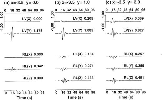
Displacement waveforms of the Love (two upper traces) and Rayleigh (three lower traces) waves at three surface points subjectto SH-wave incidence propagating in the positive direction of the x-axis in the model shown in Fig.16. The time histories are convolved with a Ricker wavelet having a centre frequency of 0.2Hz. The location of the surface points is as follows: (a) (x, y)=(− 3.5, 0), (b) (− 3.5, 1) and(c) (− 3.5, 2)km.
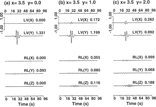
The same as Fig.19, but at three other surface points: (a) (x, y)=(3.5, 0), (b) (3.5, 1) and (c) (3.5, 2)km.
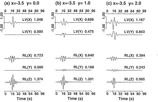
The same as Fig.19, but subject to SV-wave incidence.
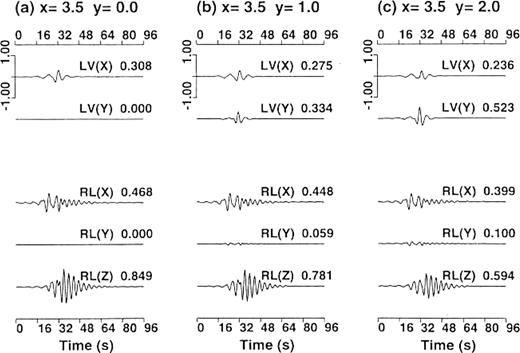
The same as Fig.21, but at three other surface points: (a) (x, y)=(3.5, 0), (b) (3.5, 1) and (c) (3.5, 2)km.
5 Discussion
Hisada (1993) (abbreviated to HS below) proposed a method similar to ours. There is an important difference with respect to the truncation between their method and ours: the former merely truncates the boundary, while the latter compensates for the truncation by the reference solution approximation. We point out two problems with simple truncation. First, simple truncation makes it ambiguous as to which basin model is assumed. HS seem to have regarded neglected boundaries as extensions of considered boundaries in the tangential direction at truncation points (e.g. Fig.4 in HS), but they did not prove this. In contrast, we explicitly showed which part of the boundaries is compensated for the truncation, and as a consequence the considered model is obvious. Second, no compensation for the truncation causes serious errors, as shown in Sections 2 and 4. Nevertheless, HS successfully simulated the secondary Love waves observed in the Kanto basin, considering part of the basin boundary truncated at certain points. This is due to the fact that a point source was used. For the point source, we can expect that the integrals over neglected boundaries away from the source will be trivial because of the decay of incident energy with distance. We here emphasize that simple truncation does not always work well when the neglected integrals are not always negligible. In fact, plane-wave incidence is a case in point, where the incident energy is distributed infinitely in space. Such cases can include the situation where basin boundaries have to be truncated at not so distant points from seismic source faults adjacent to basins. In this paper, we presented a systematic technique using the reference solution approximation: the 3-D wavefield requires compensation by the 2.5-D solutions, and the 2.5-D wavefield requires compensation by the 1-D solutions; in particular, the 3-D using wavefield for horizontally closed basin models requires compensation directly by the 1-D solutions.
In this study, we calculated only the surface waves secondarily excited on basin boundaries. We here discuss the possibility of theory allowing for multiple reverberations of the surface waves. From the theoretical point of view, our theory will apply to the reverberation problems In point of fact, however, the computer performance makes it difficult. As described in Section 3.2, we make use of the 2.5-D wavefield to compensate for the truncation of the basin boundary surface. The numerical procedure that we adopted to solve the 2.5-D wavefield was time-consuming. When we calculate the excited waves subject to the plane-wave incidence or a point source, we only have to solve the 2.5-D wavefield for the incident wavefield and the necessary amount of computation is small. On the other hand, when we try to calculate the reflected waves on part of the basin boundary, many point sources are assumed on the counterpart of the reflecting boundary and we have to calculate as many 2.5-D wavefields as point sources In the case of Fig.15, the secondarily excited Love waves were represented by the summation of the waves emitted from 216 point sources distributed on half of the boundary of the disc basin. Such a time-consuming procedure prevented us from investigating the reflected surface waves. We attempted to evaluate the reflected waves without any compensation for the truncation, and this attempt ended in failure. Although our technique succeeded only in evaluating the excited surface waves, it will be useful in interpreting the observed surface wavefield with the calculated waveforms, advancing from the stage of waveform fitting.
In calculating the Green's functions for flat-layered half-spaces using the discrete wavenumber technique, we added a small imaginary number to frequencies to avoid surface-wave poles on integration paths (Phinney 1965). This brings some attenuation and we can exclude it in the time domain. In this study, however, we did not follow the procedure to retrieve perfect elasticity in obtaining the BEM solutions on boundaries, because it results in reducing the accuracy of solutions. On the other hand, in calculating the surface waves, we used the Greens' functions represented by normal-mode summation for perfectly elastic media. In solving eigenvalue problems, we adopted a manner of searching the horizontal-wavenumber domain based on the global matrix approach and eigenvalues can be found along the real axis. However, if we take attenuation into account, we have to search the complex-wavenumber domain and this requires enormous effort. In consequence, the Q-values cannot be defined in our numerical experiments. There is the possibility of introducing attenuation to surface waves, for example using the thin-layer finite-element method (Fujiwara 1996b,c).
6 Conclusions
We presented a new numerical method to evaluate the excitation of secondary surface waves in 3-D sedimentary basin models based on the direct BEM with vertical boundaries and normal modes. We used the reflection and transmission operators defined in the space domain to prove that it is possible in principle to extract surface waves excited on parts of basin boundaries from the total 3-D wavefield. We then realized the extraction in the BEM algorithm, newly introducing the reference solution approximation technique using the 2.5-D and 1-D wavefield for reference media. This technique generally overcomes the problems arising from the truncation of boundary surfaces in the 3-D space.
We calculated the secondary Rayleigh and Love waves excited on the arc shape (horizontal section) of a vertical basin boundary subject to incident SH and SV plane waves propagating perpendicularly to the chord of the arc. As a result, we found that in the SH-incidence case the Love waves are excited predominantly, rather than the Rayleigh waves, and that in the SV-wave-incidence case the Love waves as well as the Rayleigh waves are excited. This explains the observation that Love waves are more frequently found than Rayleigh waves in the horizontal components inside sedimentary basins.
Acknowledgements
KH would like to express his gratitude to Prof. Kojiro Irikura and Dr Tomotaka Iwata for their useful advice and encouragement. Dr Yoshiaki Hisada kindly gave us useful advice about numerical integration on discretized boundary elements. Prof. Michel Bouchon and Dr Francisco Luzön kindly read this manuscript and provided valuable comments. The authors appreciate helpful comments and suggestions by two anonymous referees.
References
Appendices
3 APPENDIX A: Definition of the integ-ral operators in eqs () and (4)
80 APPENDIX B: Definition of the integral operators in eqs () to (82)

Author notes
Now at: National Research Institute of Fire and Disaster, Fire and Disaster Management Agency, Ministry of Home Affairs, 14-1, Nakahara 3-chome, Mitaka, Tokyo 181, Japan.
