


Summary
Spectral analyses of long magnetic anomaly profiles of Cretaceous age in the Phoenix and Hawaiian lineations within the Pacific Basin show two to five non-harmonic wavelength peaks, with probabilities >90 per cent, within the range of several tens to hundreds of kilometres for each profile. For each profile with four peak wavelengths, their ratios correlate strongly (r >0.98) with the ratios for the Earth's orbital eccentricity periodicities for this time, and hence the profile peaks necessarily correlate with each other. These observations suggest that the magnetic anomaly signal is influenced by the Earth's changing orbital parameters, probably through their influence on the internal geomagnetic field. This implies that assumptions usually made to convert the magnetic signal to the magnetization of the oceanic crust may be suspect. The observations, if confirmed, indicate that orbital periodicities can assist in improving the age calibration of the global polarity timescale and that the predicted orbital behaviour of the Earth is confirmed for the last 150Ma.
Introduction
In a previous paper (D'Argenio, Iorio & Tarling 1996) it was shown that the South Atlantic Cenozoic magnetic anomaly profiles synthesized by Candé & Kent (1992) and the raw magnetic readings of the intensity of Cenozoic magnetic anomalies along long profiles in the South Atlantic have similar spectral characteristics. Spectral peak wavelengths were identified for different age-range sections of the Cenozoic profiles which could be converted, using the Candé & Kent (1992) timescale, into the time domain. The periodicities in the magnetic anomalies were found to be very similar to the predicted Earth's orbital parameters for the Cenozoic (Fischer, De Boer & Premoli Silva 1990; Berger, Loutre & Laskar 1992). The present study extends the analysis to determine the spectral content of long Cretaceous magnetic anomaly profiles crossing the Phoenix and Hawaiian lineations in the Pacific (Fig.1) and then compares the spectral signatures with the predicted orbital periodicities for that time (Berger 1977; Fischer et al. 1990; Berger et al. 1992). Consideration of the causes of such cyclicities will be discussed elsewhere (Tarling, Iorio & D'Argenio, in preparation) as other relevant features arise from the magnetic signals, which are still being verified, from a continuous bore core of Lower Cretaceous carbonate sequences (Iorio 1995; Iorio et al. 1995, 1996; Brescia et al. 1996; Iorio, Tarling & D'Argenio 1998).
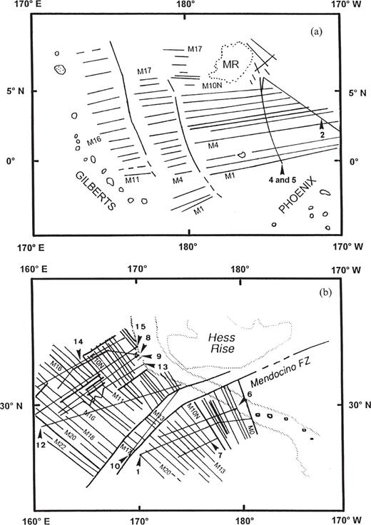
The locations of the anomaly profiles for (a) the Phoenix and (b) the Hawaiian lineations (modified from Larson & Sager 1992). Particular ocean floor anomalies are marked conventionally as M1 , M4, …, etc. Numbers not preceded by M identify the analysed profiles.
The uncertainty in dating reversals of geomagnetic polarity is far greater for the Cretaceous than for the Cenozoic (Gradstein et al. 1994). There are fewer radiometric dates available to provide ‘golden spikes’ between which the ages of other features are interpolated. There are also fewer polarity chrons identified as this time interval is dominated by the long Cretaceous normal polarity superchron. Gradstein et al. (1994) undertook a detailed re-appraisal of the Gaussian errors in the radiometric dates of appropriate biostratigraphic boundaries and polarity chronozones and used these to produce a global polarity timescale for this period. Channell et al. (1995) also produced a revised timescale for this period. Both timescales provide a considerable advance but, as pointed out previously (Tarling 1983), there are additional non-Gaussian errors present that are necessarily excluded from such revisions as they are largely unquantifiable, but not insignificant. These errors, estimated as 1–5Ma, arise mainly from uncertainties in the stratigraphic correlations between land and marine sequences. The magnitude of such errors and the Gaussian radiometric errors are far greater than the implied errors in quoting interpolated boundaries to 0.01 or 0.001Ma Huestis & Acton 1997). More significantly, they may well give rise to apparent changes in sea-floor spreading rates which are, in reality, within the known error limits of the dating. While continuing improvements in biostratigraphic and radiometric dating will gradually lead to further improvements in the global polarity timescale, an independent method of assessing the reliability of the dating, such as the use of astronomical periodicities, could prove of considerable value in the earth sciences.
Methods And Techniques
As in the earlier study (D'Argenio et al. 1996), magnetic anomaly profiles were selected, as far as possible, in regions well away from known later volcanic activity and tectonic disturbance and where sea-floor spreading appeared to have been fairly constant during the time represented by the profile. The South Atlantic study had shown that the higher spectral frequencies could only be determined when the magnetometer reading rates had been reasonably rapid, relative to the rate of sea-floor spreading involved, and the speed of the ship. On this basis, long profiles were selected where the magnetometer readings had been recorded at least every 5min along track. Using these criteria, 13 profiles (Table 1) were eventually chosen from many examined in the CD databases of the Global Database (NGDC Marine Geological & Geophysical Data 1993). Only seven profile tracks could be found that largely fulfilled these criteria and were also essentially perpendicular to the strike of the magnetic anomalies (Fig.1). The other six profiles, termed subperpendicular, fulfilled most criteria, but were at angles of 15° or more to the sea-floor-spreading flow-line, and some contained changes in the ships’ tracks. The total anomaly range extended from anomalies M0 to M21. In all cases, the data were fairly old and poorly located compared with the latest techniques. Nonetheless, such uncertainties are small compared with the smoothing effects resulting from the readings being made at sea level, some 5km above the ocean floor in these profiles.
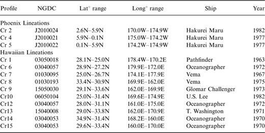
Sources and locations of the data.
The method of analysis was the same as for the South Atlantic Cenozoic anomalies. The anomaly field readings were used or determined by removing the appropriate International Geomagnetic Reference Field values from the raw readings. [No other processing was undertaken as this would require assumptions concerning the origin and nature of the remanence generating the anomaly fields (Harrison 1987).] The spectral content of each profile was then determined using the FFT method based on the Modified Scargle algorithm Horne & Baliunas 1986) as described by D'Argenio et al. (1996) and Brescia et al. (1996). This method deals with unevenly spaced data, minimizes aliasing and provides a direct probability estimate (the ‘false alarm’ probability). Spectral leakage was reduced by means of a window function prior to the analyses. Each anomaly profile was analysed in the space domain (Table 2 and Figs 2–14). Only peak values with a probability greater than 90 per cent were accepted for further consideration; peaks related to the length of the data set were eliminated by the software and harmonics of the peaks were manually excluded. (The most evenly spaced data sets were also analysed, using the FFT algorithms of the Origin© program, as an independent check of the method. This yielded essentially identical results but is less appropriate for irregularly spaced data.) The anomaly peak wavelengths are described below in numerical order as given in Table 2.
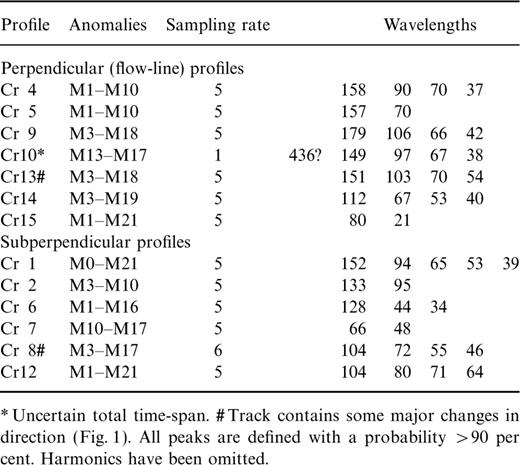
The spatial spectral peaks (km) identified along the different profiles.
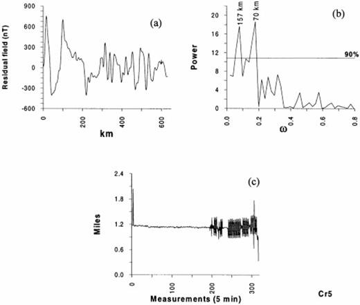
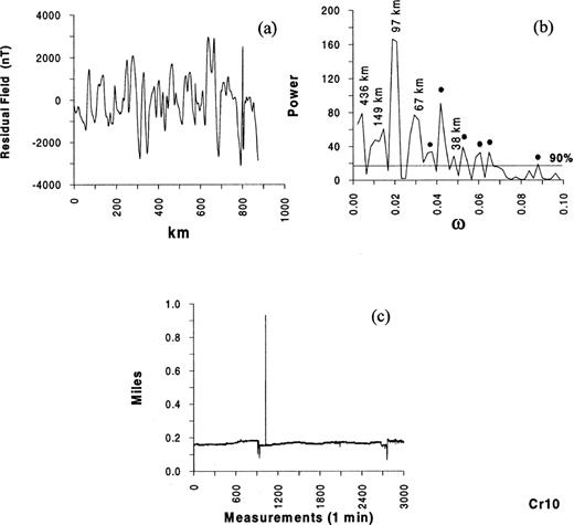
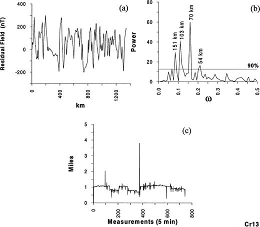
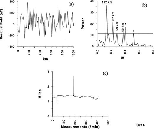
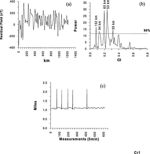
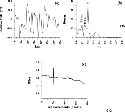
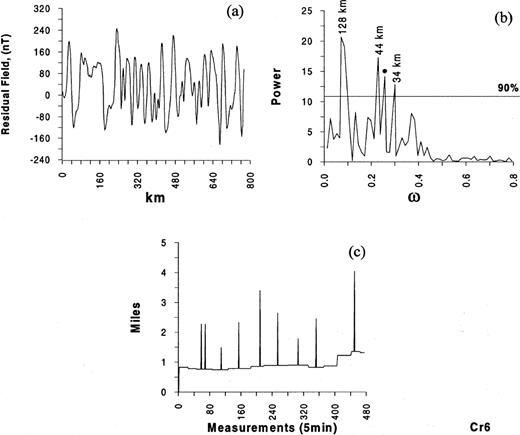
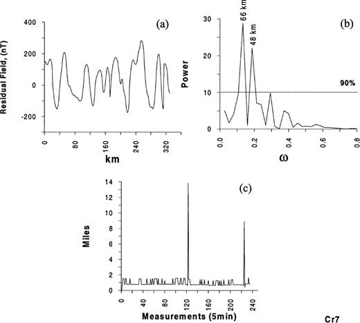
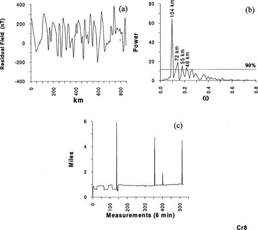
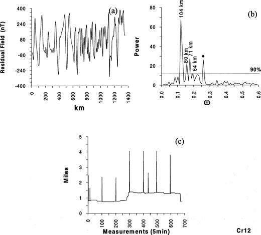
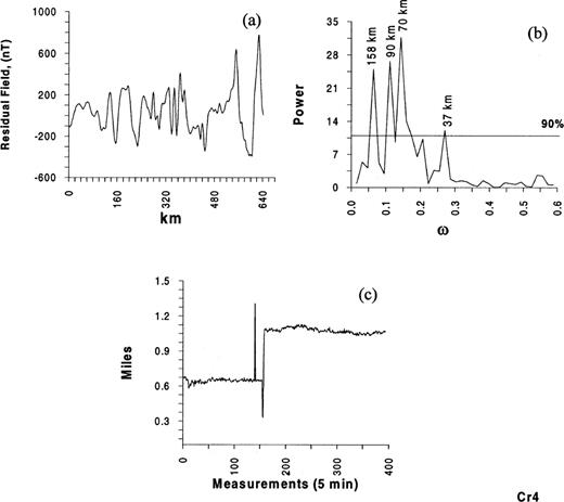
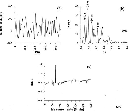
Profile Cr 4. (a) The anomaly profiles (nT). (b) The spectral analysis based on Horne & Baliunas (1986). The horizontal line marks the line above which the peaks are defined with a probability >90 per cent. Peaks above this line are labelled with their median wavelength value unless they appear to be harmonics, in which case they are marked with a dot. (c) The magnetometer-reading frequency (reading per minute).
Profile Cr 10. Legend as Fig.2.
Profile Cr 13. Legend as Fig.2.
Profile Cr 14. Legend as Fig.2.

Profile Cr 15. Legend as Fig.2.
Profile Cr 1. Legend as Fig.2.
Profile Cr 2. Legend as Fig.2.
Profile Cr 6. Legend as Fig.2.
Profile Cr 7. Legend as Fig.2.
Profile Cr 8. Legend as Fig.2.
Profile Cr 12. Legend as Fig.2.
Results
Perpendicular profiles
Phoenix profile Cr4 (Fig.2)
This had a slightly arcuate track relative to the anomaly strike, but was largely perpendicular to it. Two separate, but very consistent, reading rates were involved, although the change in reading rate was not evident in the anomaly profile. Spectral analysis showed four spectral peaks of which three were particularly well defined.
Phoenix Profile Cr5 (Fig.3)
Profile Cr 5. Legend as Fig.2.
This followed the same track as Cr4, except for a short distance at the end, and had a mostly constant reading rate except for the last third of its length. Two spectral peaks were clearly identified.
Hawaiian Profile Cr9 (Fig.4)
Profile Cr 9. Legend as Fig.2.
The profile was parallel to, and between, profiles Cr15 and Cr13 and was almost exactly perpendicular to the anomaly strike. The reading rate remained very constant along the total profile. Six spectral peaks were very clearly defined, of which two were rejected as being harmonics.
Hawaiian Profile Cr10 (Fig.5)
The track was almost exactly perpendicular to the anomaly stripes and the reading rate was virtually constant throughout the profile. The paucity of identified anomalies at the beginning and end of the profile makes the total time span uncertain. The spectral analysis shows many very well-defined peaks of which six are harmonics. The longest-wavelength peak, 436km, is discounted as necessarily being poorly defined as only two wavelengths could be involved in its determination. There are thus four primary peaks.
Hawaiian Profile Cr13 (Fig.6)
While most of this track was perpendicular to the anomaly pattern, there were marked changes in the ship's direction in the centre of the profile. The reading rate was constant throughout. Four peaks were identified, mostly well above the surrounding spectral noise, none of which was a harmonic.
Hawaiian Profile Cr14 (Fig.7)
The profile was close to perpendicular to the anomaly pattern for most of its length, but appears to have crossed a fracture zone at its western extremity. The reading rate was constant. Six peaks were identified, mostly well above the surrounding spectral noise, of which two peaks were harmonics.
Hawaiian Profile Cr15 (Fig.8)
The profile appears to have been at only a slight angle to the flow-line for most of its length and the reading rate was reasonably consistent. Only four spectral peaks were identified, of which two were harmonics.
Subperpendicular profiles
Hawaiian Profile Cr1 (Fig.9)
The start and end of this profile were well defined, but there was one major change in direction, with both tracks being subperpendicular to the anomaly pattern. The reading rate was constant. Five peaks were clearly identified.
Phoenix Profile Cr2 (Fig.10)
This profile covered similar anomalies to Cr4 and Cr5, but at a far greater angle to their strike. The reading rate was reasonably constant along the profile. Three peaks were identified, of which the best defined was a harmonic.
Hawaiian Profile Cr6 (Fig.11)
The track of this profile was subperpendicular to the anomaly pattern, although the anomalies were fanning slightly relative to the line of the profile. The reading rate was constant. Four peaks were identified, of which one was a harmonic.
Hawaiian profile Cr7 (Fig.12)
The track was parallel to and south of profile Cr6, but of shorter length. The reading rate was fairly constant. Two very well-defined peaks were identified.
Hawaiian Profile Cr8 (Fig.13)
The track of this profile, mostly between Cr15 and Cr14, involved two major changes in direction, and had a consistent reading rate. Four peaks were identified, none of which was a harmonic.
Hawaiian Profile Cr12 (Fig.14)
This was the longest profile and was straight, but crossed the anomaly stripes at angles up to about 45° as well as possibly crossing unidentified fracture zones and fan-shaped anomaly patterns in the east. The readings were at two different, but constant, rates. Five very well-defined peaks were determined, of which one was a harmonic.
Comparisons
Several of the profiles contain irregularities in their orientations and a few appear to cross unrecognized features that may have disturbed the anomaly signatures. Nonetheless, at least two, mostly four, peaks of coherent wavelengths have been identified on each profile, indicating the presence of coherent signals on all profiles. The most consistent profiles were Cr10 and Cr9; both had near-constant reading rates, were of similar length and were essentially ‘flow-line’ tracks. They both showed very clear spectral peaks that were also similar to each other (Figs 4 and 5), but such comparisons may be uncertain as the profiles are separated by more than 500km and at least two fracture zones. Consequently, they are likely to have had different spreading rates. A better assessment of the consistency of the analyses is provided by comparing those parts of the two Phoenix profiles, Cr4 and Cr5, that are along an identical track, the former moving from north to south and the latter in the reverse direction and being truncated to enable direct comparison. However, both tracks are arcuate relative to the anomaly strike and therefore change angle relative to the flow-line. Both anomaly profiles show strong similarities, being close to mirror images of each other (cf. Figs 2 and 3). It is thus not surprising that two peaks on each profile are virtually identical, 158:169km and 70:70km, while the Cr4 90km peak corresponds to a similar Cr5 peak at 104km, although the latter has been discounted as not being defined with a probability >90 per cent. The similarities between Cr9 and Cr10 and between Cr4 and Cr5 are therefore strong, suggesting that the errors in determining the individual peaks may be less than 5 per cent. There is no way to evaluate adequately the extent to which similar discrepancies occur on other profiles, but the profile assessed as being nearest to a flow-line, known to cover the widest anomaly age range, least affected by later geological events and with a consistently high reading rate, Cr10, shows peaks that have much higher probability levels than the other profiles. For all profiles, most peaks with probabilities greater than 90 per cent are well defined and have height to width ratios exceeding 9. There is thus no doubt about the existence of coherent signals within the range of a few tens to a few hundredof kilometres. The noise in the analysis mostly originated from the depth of the magnetic sources relative to the magnetometer and from the tracks examined having been largely planned to define these magnetic anomaly patterns in the Pacific; it was clearly impossible to plan flow-line profiles until such pioneer work had been completed.
As the different profiles represent different times and different rates of spreading, the consistency of the peak wavelengths between different profiles cannot be compared directly without some form of normalization, such as comparison of the ratios between the peaks. It is not immediately obvious which peak wavelength should be used for this normalization and it is also suspected that some peaks are derived from a single split peak, e.g. Cr12. The short wavelengths should be best defined in the analysis as the number of wavelengths per profile will be higher, but these are also likely to be most affected by changes in reading frequency. It was decided to use only those profiles with four peaks as this increased the reliability of any correlation assessment, although more than a third of the profiles had to be omitted. However, the ratios are all proportional, irrespective of the choice of normalization peak, so the seven profiles containing four peaks were considered and normalization was made against their shortest identified peak wavelength (Table 3). As the South Atlantic study had indicated the presence of astronomical periodicities in the Cenozoic data, comparison was also made directly with the ratios of the Earth's orbital eccentricity periodicities (3400, 2030, 1290 and 400ka) predicted for this period (Berger 1977; Fischer et al. 1990; Berger et al. 1992). In all cases, the correlation coefficient, r, between each profile anomaly ratios and the predicted eccentricity periodicities had a value of at least 0.98, with the marginally higher correlations associated with the more perpendicular profiles. None of the excluded profiles, that is those with more or fewer than four identified wavelength peaks, was inconsistent with the same conclusion, but their inclusion involved subjective matching of particular peaks and thus detracted from the objectivity of the analysis.
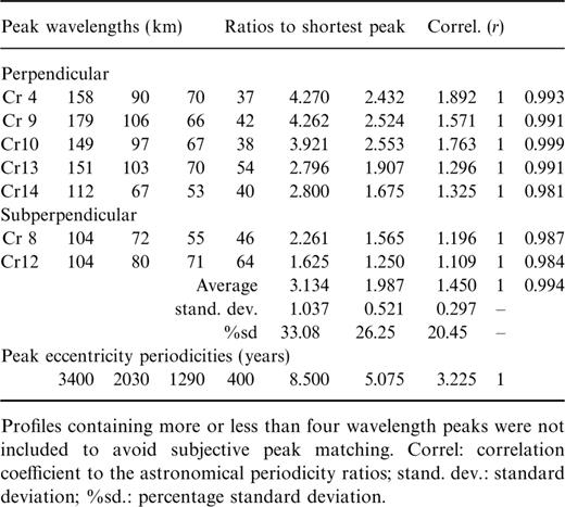
Comparisons and correlations of peak wavelength ratios and the Earth's predicted eccentricity periodicity ratios.
Comments And Conclusions
The main feature of this study is that, when no assumptions are made concerning the nature of the remanence, there are consistent wavelengths, on all profiles, which have probabilities greater than 90 per cent and are mostly distinct, that is they have high height to width ratios. Where four peaks are present, their ratios show very high correlations with those of the four main periodicities of the Earth's eccentricity for the Cretaceous. Clearly, such correlations are not necessarily causative as they only indicate the presence of similar wavelength ratios, but it seems most probable that the observed wavelengths are related to the nature and orientation of the magnetization of the oceanic crust and that this, in turn, will be affected by the long-term behaviour of the geomagnetic field. This will be discussed (Tarling, Iorio and DȧArgenio, in preparation) after examining independent evidence for a correlation between geomagnetic parameters and astronomical periodicities in Cretaceous bore cores from southern Italy (Iorio 1995; Iorio et al. 1995, 1996; Brescia et al. 1996; Iorio, Tarling and D'Argenio 1998). At this stage, it is thought that at least some of the features of these anomaly records can be explained most readily if the Earth's poloidal magnetic field is directly affected by the Earth's orbital frequencies, as suggested by Malkus (1963). The results also indicate that some of the basic assumptions about the nature of the magnetization of the oceanic crust (Harrison 1987), conventionally made when processing magnetic anomaly data to derive geomagnetic field behaviour, may well be invalid and require a re-evaluation (Tarling, Iorio and D'Argenio, in preparation).
At this stage, the available ocean magnetic anomaly records alone are inadequate to test between the different polarity timescales for this period (Harland et al. 1990; Gradstein et al. 1994; Channell et al. 1995). Further developments should, however, enable the evaluation of the reality of many suggested accelerations and decelerations of global or plate-wide sea-floor spreading. The agreement between the wavelength peaks and Berger et al.'s (1992) predictions for the astronomical periodicities also suggests that changes in palaeogeography and postulated cometary impacts have not had a significant effect on at least the Earth's orbital eccentricity parameters (Tarling, D'Argenio & Iorio 1997). However, deep-tow magnetometer profiles along sea-floor-spreading flow-lines are necessary to enable a full evaluation of the basic assumptions made concerning the nature and origin of the magnetization of the oceanic crust, to determine the relationship between the anomalies and internal core processes and, ultimately, to provide an astronomically calibrated global polarity timescale.
Acknowledgements
This paper was carried out with the financial support of Research Institute ‘Geomare Sud’ CNR. The database related to this work has been processed and interpreted by MI. The geological interpretation and the conclusions stem from discussions amongst all of the authors, assisted by a Short Mobility Term, 1997, grant from the National Research Council of Italy.
References
