Correcting Bias in Allele Frequency Estimates Due to an Observation Threshold: A Markov Chain Analysis

Abstract

There are many problems in biology and related disciplines involving stochasticity, where a signal can only be detected when it lies above a threshold level, while signals lying below threshold are simply not detected. A consequence is that the detected signal is conditioned to lie above threshold, and is not representative of the actual signal. In this work, we present some general results for the conditioning that occurs due to the existence of such an observational threshold. We show that this conditioning is relevant, for example, to gene-frequency trajectories, where many loci in the genome are simultaneously measured in a given generation. Such a threshold can lead to severe biases of allele frequency estimates under purifying selection. In the analysis presented, within the context of Markov chains such as the Wright–Fisher model, we address two key questions: (1) “What is a natural measure of the strength of the conditioning associated with an observation threshold?” (2) “What is a principled way to correct for the effects of the conditioning?”. We answer the first question in terms of a proportion. Starting with a large number of trajectories, the relevant quantity is the proportion of these trajectories that are above threshold at a later time and hence are detected. The smaller the value of this proportion, the stronger the effects of conditioning. We provide an approximate analytical answer to the second question, that corrects the bias produced by an observation threshold, and performs to reasonable accuracy in the Wright–Fisher model for biologically plausible parameter values.

conditioned observations, missing values, random genetic drift, Wright–Fisher model, population genetics theory, stochastic population dynamics

Significance

The occurrence of signals with undetectable values is common in biological data. A possible consequence of this is a severe bias in the observed data. Here we focus on the implications, primarily for allele frequencies, of the situation where a biological signal, such as the count of a number, can only be detected when it lies above a threshold level. When there is such an observation threshold, the signal detected is not representative of the actual signal, but corresponds to a signal that is conditioned to lie above threshold. This conditioning is explicitly shown to have an appreciable effect on measurable quantities and needs to be fully taken into account in the analysis of biological data. In a mathematical analysis of this problem, we (1) determine a natural measure of the strength of the conditioning associated with an observation threshold, and (2) determine an approximate way to correct for the effects of the conditioning.

Introduction

There are many problems in biology and related disciplines involving stochasticity, that is, randomness that unfolds over time, where the detection of a non-negative signal (such as a number) can be made only when the signal lies above a threshold level. When there is such an observation threshold, we assume that a signal with a value below threshold, at the time of observation, is not detected. Alternatively, if the signal has a value above threshold then it can be detected and recorded and used in analysis. Importantly, the values of a signal that are detected, when there is an observation threshold, are not representative of the actual signal, but correspond to a signal that is conditioned to lie above the threshold level.

Detecting and quantifying signals with an implicit threshold, that lead to missing (or non-observed) values are widespread in biological data, such as label-free mass spectrometry (Karpievitch et al. 2009, 2012). A possible consequence of missing values are severe biases, although their systematic impact is often unclear (Välikangas et al. 2018). Generally missing values in biological measurements can be roughly divided into two types: (1) abundance-dependent missing values (e.g., due to a detection limit of an instrument), and (2) values missing at random (e.g., erroneous non-identification). However, distinguishing between these two types of missing values is far from trivial. To address the missing value problem in biological data various methods of data imputation have been proposed (Webb-Robertson et al. 2015), but these methods themselves may introduce additional biases (Välikangas et al. 2018).

Missing values, as a result of observation thresholds, are not only common to proteomics, but also apply to next-generation sequencing data. For example, observation thresholds become relevant when the amount of a biological sample or the sequencing depth is low, as occurs in metagenomics (Hildebrand et al. 2019), single-cell transcriptomics (Yang et al. 2018), genome re-sequencing approaches (Kim et al. 2011; Nielsen et al. 2011; Chan et al. 2016; Barghi et al. 2019) and ancient DNA (Loog et al. 2017). If not taken into account, missing values may lead to severe biases in subsequent population genetic analyses, as occurs, for example, when a large number of data points are excluded (Hughes et al. 2008; Stoletzki and Eyre-Walker 2011). Correcting for missing values and the resulting biases may, however, be possible, but has typically been dealt with using methods tailored to the particular problem at hand (Rimmer et al. 2014; Han et al. 2015).

Due to advances in DNA sequencing, the availability of time-series data has become increasingly common (Malaspinas et al. 2012). Extensive time-series data presents the opportunity for more efficient methods of detecting selection, due to the link between allele frequency trajectories and the strength of selection (Bollback et al. 2008). As a result of this, likelihood-based methods have been developed to co-estimate selection coefficients and the effective population size (Bollback et al. 2008; Foll et al. 2015; Shim et al. 2016). Additionally, Bayesian approaches have been developed to detect targets of selection from evolve-and-resequence experiments (Schraiber et al. 2016; Barata et al. 2020).

Gene frequency trajectories may be used to trace the fate of an individual mutation, or a set of mutations, in a time-dependent manner, in order to identify the underlying selective regime (Gossmann et al. 2014; Shafiey et al. 2017). The behavior of gene frequency trajectories is determined by the interplay of deterministic and random evolutionary “forces” and various conclusions can be drawn from knowledge of such trajectories. However, suppose we have limited knowledge of a gene frequency trajectory. As an example, suppose we know the initial frequency of an allele (in, say ancient DNA, Dehasque et al. 2020), and we know the frequency of the allele in extant organisms, which is the final frequency of the trajectory. This knowledge, limited as it is to initial and final frequencies, amounts to a form of conditioning of the trajectory (also described as “ascertainment” in the literature, Marth et al. 2004) that may strongly influence our estimates of the trajectory at intermediate times and its overall shape. Indeed, conditioning trajectories, by restricting considerations to only trajectories with known initial and final frequencies, has been previously shown to be indistinguishable from the action of an additional evolutionary force, which may be interpreted as a contribution to the selection that is acting (Zhao et al. 2013). Furthermore, this “conditioning induced additional selection” can easily be comparable with the actual selection that is acting (Zhao et al. 2013; Shafiey et al. 2017). Closely related to this, is the conditioning that arises from an observation threshold, where the only frequency trajectories that contribute to any analysis are those whose final frequency lies above a threshold. The trajectories whose final frequency lies below threshold are not observed, and are effectively discarded. This “threshold conditioning,” if not taken into account, may lead to appreciable distortions of the inferred behavior of such trajectories, and may confound estimates of biologically relevant parameters that characterize the dynamics. Generally, threshold conditioning needs to be fully taken into account in the analysis of biological data.

In this work, we focus on the implications, for allele frequencies, of the conditioning associated with an observation threshold. We restrict our considerations to systems that can be described as Markov chains. These are “memoryless” systems in which only knowledge of the present state of the system (and not that of past states), influences future behavior. Standard models of genetics, such as the Wright–Fisher model (Fisher 1930; Wright 1931), are Markov chains.

In this work, we address the following two key questions.

What is a natural measure of the bias of estimates that results due to an observation threshold?
What is a principled way to correct for the bias of results arising from an observation threshold?

The overall structure of this paper, that leads to the answers to these questions, is as follows.

The main text begins with a presentation of the theory associated with an observation threshold, which we give in a somewhat general setting, due to the possible applicability of this work in different areas. A crucial role is shown to be played by $P_{det}$ ⁠, the probability that a detectable (i.e., above threshold) result will be obtained at the time of observation. An alternative interpretation of $P_{det}$ is that it is the proportion of a large number of trajectories of the system (for example frequency trajectories) which exceed the threshold value at the time of observation. We discuss $P_{det}$ in a section that deals with its importance as a natural measure of the bias that results, due to the existence of a threshold. We then show how $P_{det}$ can be used to approximately correct results that have become biased in value, because of the threshold.

Next, we illustrate the usage of the theory in the context of a model of population genetics. We carry out simulations of a population that is subject to a threshold such that trajectories associated with focal alleles are unobservable if they lie below a threshold frequency. This is then followed by a section where the Wright–Fisher model is analysed, to show in some detail the effects of a threshold and we present a statistical analysis that illustrates the use of $P_{det}$ to correct frequency observations made in the presence of a threshold. The main text concludes with a discussion, where application of this work to real data is illustrated. Three appendices contain mathematical details of the theory presented in this work.

Theory

While there may be other interpretations of this work, we shall discuss the conditioning associated with an observation threshold using language and notation appropriate to trajectories of a system. Thus we assume the system is described by a discrete numerical value of a measurable quantity, which randomly changes over time (thereby constituting a stochastic process). With t denoting the time, and $M (t)$ denoting value of the measurable quantity at time t, a trajectory is simply the set of values that $M (t)$ takes over a range of times. For example, if $M (t)$ corresponds to the number of copies of an allele in a population at time t, then a trajectory in this case corresponds to the set of values that this number sequentially achieves over a range of times.

The conditioning we consider in this work represents limitations, at a given observation time, on what can be observed about a Markov chain (i.e., a “memoryless” stochastic process Tuckwell 1995). In terms of trajectories of the system, conditioning can be viewed as there being a subset of trajectories that are not observable because they fail to satisfy a particular condition. Generally, statistical effects and implications of conditioning emerge by computing statistics of interest from only the subset of trajectories that satisfy the particular condition and hence are observable (thereby yielding conditioned statistics).

We shall next give results for a class of conditioned problems for discrete state/discrete time Markov chains. Related results (not presented) apply to continuous state/continuous-time diffusion processes, since there are very close mathematical relations between the discrete and continuous problems. Indeed, a diffusion process is a well-known continuous state/continuous-time process that is a very natural and reasonable approximation of a standard discrete state Markov chain of population genetics, namely the Wright–Fisher model (Kimura 1964).

Markov Chain Model

Consider a discrete state, discrete time Markov chain, where times are given by $t = 0, 1, 2, \dots,$ and state labels are integers that can take the finite range of values $0, 1, 2, \dots, N$ ⁠. We shall often use the letters n and m for state labels.

Let $M (t)$ denote a random variable that represents the state of the system at time t. Thus $M (t)$ takes one of the values $0, 1, \dots, N$ ⁠.

We assume that the label used to describe the state of the Markov chain is proportional to a measurable quantity such as a frequency, a number or a position, and in what follows, we shall not distinguish between the label of the state (state for short), and the value of the associated measurable quantity. Then states that lie below threshold (sub-threshold states) are associated with a small value of the measurable quantity. We consider the situation where, at an observation, only values of the measurable quantity/state of the system that exceed the value z can be detected. If the state of the system is z or smaller than the measurable quantity will not be detected. We term z the threshold value.

We work under the assumptions that: (i) at an initial time of 0 the system is described by a known distribution (or is in a known state), and (ii) at a later time, termed the observation time and denoted by $t_{obs}$ ⁠, the state of the system is measured/observed.

Let us describe the random variable representing the state of the system at time t, namely

M (t)

⁠, in probabilistic terms. For

u \leq t

let

K_{m, n} (t | u)

denote the probability that

M (t)

takes the value m (i.e., that

M (t) = m

⁠), given that at earlier time, u, it took the value n (i.e.,

M (u) = n

⁠). Thus

K_{m, n} (t | u) = Prob [M (t) = m | M (u) = n]

⁠. It is convenient to write this probability as the

(n, m)

element of an

(N + 1) \times (N + 1)

matrix

K (t | u)

and we use the notation

K_{m, n} (t | u)

[K (t | u)]_{m, n}

to denote the matrix element. The matrix

K (t | u)

changes according to the rule

K (t + 1 | u) = W (t) K (t | u)

(1)

where

W (t)

is the transition matrix of the Markov chain at time t. The transition matrix governs changes of state between the times t and

t + 1

⁠, and the

(m, n)

element of this matrix is given by

W_{m, n} (t) \equiv [W (t)]_{m, n} = Prob [M (t + 1) = m | M (t) = n]

(Tuckwell 1995).

Probability of an above Threshold Result

For the form of conditioning considered here, a basic quantity of interest is the probability that a detectable result will be obtained at time

t_{obs}

⁠. We write this probability as

P_{det}

⁠. It is the probability of the system achieving a state that lies above threshold at time

t_{obs}

and we can write

P_{det} = Prob [M (t_{obs}) > z] .

(2)

Another interpretation is that

P_{det}

is the proportion of a large number of trajectories of the system whose value, at time

t_{obs}

⁠, exceeds the threshold value, z.

Throughout this work, we shall make the assumption that

P_{det}

lies in the range

0 < P_{det} < 1

(3)

which corresponds to some, but not all, of a large number of trajectories, being above threshold at the observation time.

Proceeding, let the initial distribution of states of the system be given by the column vector

Φ (0)

⁠, whose mth element, written

Φ_{m} (0)

⁠, is the probability that

M (0) = m

⁠. In Appendix A we show that in terms of the quantity

Q_{m}

defined by

Q_{m} = \sum_{b > z} K_{b, m} (t_{obs} | 0)

(4)

we have

\begin{aligned} P_{det} & = \sum_{m = 0}^{N} Q_{m} Φ_{m} (0) general case \\ = Q_{a} special case \end{aligned}

(5)

where the general case applies when a set of states, as described by

Φ (0)

⁠, have a non-zero probability to occur at time 0, while the special case applies when only state a occurs at time 0.

We note that $P_{det}$ ⁠, by its definition (eqs. 4 and 5), depends on $t_{obs}$ ⁠, z, and $Φ (0)$ ⁠. In addition $P_{det}$ depends on the parameters that characterize the Markov chain and hence characterize the behavior of $M (t)$ ⁠.

We shall provide numerical examples of $P_{det}$ later, when we consider a specific Markov chain model of interest in population genetics.

Conditional Distribution

An unconditioned system has a probability distribution that at time t is given by

Φ (t) = K (t | 0) Φ (0)

or more explicitly

\begin{matrix} Φ_{m} (t) = & \sum_{n = 0}^{N} K_{m, n} (t | 0) Φ_{n} (0) general case \\ = K_{m, a} (t | 0) special case . \end{matrix}

(6)

As before, the general case applies when the sets of states described by

Φ (0)

can occur at time 0, while the special case applies when only state a occurs at time 0.

We show in Appendix B that when only states exceeding z can be detected at the observation time,

t_{obs}

⁠, the corresponding conditional distribution of the state of the system [equivalently the conditional distribution of

M (t_{obs})

], is given by

Φ_{m}^{cond} (t_{obs}) = {\begin{matrix} 0, & m \leq z, \\ \frac{Φ_{m} (t_{obs})}{P_{det}}, & m > z . \end{matrix}

(7)

Importance of $P_{det}$ and Retrieving Unconditioned Results

Given the unconditioned distribution of $M (t)$ at the observation time $t = t_{obs}$ ⁠, the effect of conditioning on the distribution seems fairly innocuous, namely (i) eliminate the contribution of sub-threshold states and (ii) renormalize the resulting distribution, so it is normalized to unity [this renormalization results in the presence of $P_{det}$ in equation (7)]. The conditioning, however, generally causes an increase in the expected value of $M (t_{obs})$ relative to the unconditioned value (see Appendix C), and the level of this increase can be substantial. The numerical results we give below, in figure 1 and table 1, show that when the observation threshold is $5 %$ of the maximum possible value of M, there can be more than a $50 %$ increase in the expected value of M due to conditioning. Yet larger increases, due to conditioning, can easily arise. For example, just changing the observation time used in figure 1 and table 1, from 150 generations to 300 generations, leads, approximately, to a $280 %$ increase in the expected value of M due to conditioning. There can thus be large discrepancies between statistics of $M (t_{obs})$ ⁠, which are determined from observations which incorporate effects of the threshold into their values, and the “true” statistics of $M (t_{obs})$ ⁠, which would be obtained if no such threshold existed.

Fig. 1.

Simulated replicate trajectories of a Wright–Fisher model for an asexual haploid population of size $N = 500$ ⁠. In the model, a single biallelic locus, with alleles A and B, is under selection. With $X (t)$ denoting the frequency of the A allele in generation t, all trajectories started from an initial frequency of $X (0) = a / N = 200 / 500 = 0.4$ ⁠. The selection coefficient of the A allele, relative to that of the B allele is $s = - 0.01$ ⁠, and there are equal forward and backward mutation rates of the A allele of $μ = ν = 10^{- 5}$ ⁠. The figure shows only 20 of the stochastic trajectories but 10,000 replicate trajectories were used to calculate statistics at an observation time of $t_{obs} = 150$ generations. The 10,000 replicate trajectories represent 10,000 independent loci in the hybridization scenario described in the text. A threshold, acting at a frequency of $z / N = 25 / 500 = 5 %$ ⁠, renders undetectable any of the focal loci with an A allele frequency of $5 %$ or less. For a particular simulation run, a proportion $P_{det} ≃ 0.6467$ of all 10,000 trajectories were above threshold at $t_{obs}$ ⁠, and hence were detectable. For this simulation run the unconditioned mean value of the frequency at the observation time (i.e., calculated from all 10,000 trajectories) was $E [X (t_{obs})] ≃ 0.1498$ ⁠, but the corresponding mean value, when conditioned to lie above threshold, was found to be $E_{z} [X (t_{obs})] ≃ 0.2249$ ⁠. Using $E_{est} [X (t_{obs})] = E_{z} [X (t_{obs})] \times P_{det}$ ⁠, as an estimate of the unconditioned mean frequency, leads to $E_{est} [X (t_{obs})] ≃ 0.1455$ ⁠. Thus for this simulation run, the conditioned expected value, $E_{z} [X (t_{obs})]$ ⁠, is approximately $50 %$ larger than the unconditioned result $E [X (t_{obs})]$ ⁠, while the estimated result, following from $E_{est} [X (t_{obs})]$ ⁠, differs from the unconditioned result by approximately $3 %$ ⁠. More statistics, based on this simulation run, are given in table 1.

Open in new tab Download slide

Table 1.

Open in new tab

This Table Contains Results from a Simulation of a Wright–Fisher Population with Parameters and Description as Given in the Caption of Figure 1

Quantity	Description	Value	% Error
$E [X (t_{obs})]$	Unconditioned mean frequency	$0.15$	—
$E_{z} [X (t_{obs})]$	Conditioned mean frequency	$0.22$	$50.2$
$E_{est} [X (t_{obs})]$	Estimated mean frequency	$0.15$	$- 2.9$
$E [(X (t_{obs}))^{2}]$	Unconditioned mean square frequency	$0.05$	—
$E_{z} [(X (t_{obs}))^{2}]$	Conditioned mean square frequency	$0.07$	$54.2$
$E_{est} [(X (t_{obs}))^{2}]$	Estimated mean square frequency	$0.05$	$- 0.3$
$Var (X (t_{obs}))$	Unconditioned variance	$0.03$	—
${Var}_{z} (X (t_{obs}))$	Conditioned variance	$0.02$	$- 9.3$
${Var}_{est} (X (t_{obs}))$	Estimated variance	$0.03$	$4.5$

Quantity	Description	Value	% Error
$E [X (t_{obs})]$	Unconditioned mean frequency	$0.15$	—
$E_{z} [X (t_{obs})]$	Conditioned mean frequency	$0.22$	$50.2$
$E_{est} [X (t_{obs})]$	Estimated mean frequency	$0.15$	$- 2.9$
$E [(X (t_{obs}))^{2}]$	Unconditioned mean square frequency	$0.05$	—
$E_{z} [(X (t_{obs}))^{2}]$	Conditioned mean square frequency	$0.07$	$54.2$
$E_{est} [(X (t_{obs}))^{2}]$	Estimated mean square frequency	$0.05$	$- 0.3$
$Var (X (t_{obs}))$	Unconditioned variance	$0.03$	—
${Var}_{z} (X (t_{obs}))$	Conditioned variance	$0.02$	$- 9.3$
${Var}_{est} (X (t_{obs}))$	Estimated variance	$0.03$	$4.5$

Note.—The statistics reported in the table are as follows.

Mean frequency of the A allele when:
- unconditioned (calculated from all 10,000 trajectories) and written $E [X (t_{obs})]$ ⁠,
- conditioned to lie above threshold (calculated from 6,467 above threshold trajectories, corresponding to $P_{det} ≃ 0.6467$ ⁠) and written $E_{z} [X (t_{obs})]$ ⁠,
- estimated from $E_{est} [X (t_{obs})]$ which is defined as $E_{z} [X (t_{obs})] \times P_{det}$ ⁠.
Mean square frequency of the A allele when:
- unconditioned, written $E {[X (t_{obs})]^{2}}$ ⁠,
- conditioned to lie above threshold, written $E_{z} {[X (t_{obs})]^{2}}$ ⁠,
- estimated, from $E_{est} {[X (t_{obs})]^{2}}$ which is defined as $E_{z} {[X (t_{obs})]^{2}} \times P_{det}$ ⁠.
Variance of $X (t_{obs})$ when:
- unconditioned, writing $Var [X (t_{obs})] = E {[X (t_{obs})]^{2}} - E [X (t_{obs})]^{2}$ ⁠,
- conditioned to lie above threshold, writing ${Var}_{z} [X (t_{obs})] = E_{z} {[X (t_{obs})]^{2}} - E_{z} [X (t_{obs})]^{2}$ ⁠,
- estimated, writing ${Var}_{est} [X (t_{obs})]$ which is defined as $E_{est} {[X (t_{obs})]^{2}} - {E_{est} [X (t_{obs})]}^{2}$ ⁠.

In addition, percentage errors of the conditioned and estimated results are given, relative to the unconditioned results.

Table 1.

Open in new tab

This Table Contains Results from a Simulation of a Wright–Fisher Population with Parameters and Description as Given in the Caption of Figure 1

Quantity	Description	Value	% Error
$E [X (t_{obs})]$	Unconditioned mean frequency	$0.15$	—
$E_{z} [X (t_{obs})]$	Conditioned mean frequency	$0.22$	$50.2$
$E_{est} [X (t_{obs})]$	Estimated mean frequency	$0.15$	$- 2.9$
$E [(X (t_{obs}))^{2}]$	Unconditioned mean square frequency	$0.05$	—
$E_{z} [(X (t_{obs}))^{2}]$	Conditioned mean square frequency	$0.07$	$54.2$
$E_{est} [(X (t_{obs}))^{2}]$	Estimated mean square frequency	$0.05$	$- 0.3$
$Var (X (t_{obs}))$	Unconditioned variance	$0.03$	—
${Var}_{z} (X (t_{obs}))$	Conditioned variance	$0.02$	$- 9.3$
${Var}_{est} (X (t_{obs}))$	Estimated variance	$0.03$	$4.5$

Quantity	Description	Value	% Error
$E [X (t_{obs})]$	Unconditioned mean frequency	$0.15$	—
$E_{z} [X (t_{obs})]$	Conditioned mean frequency	$0.22$	$50.2$
$E_{est} [X (t_{obs})]$	Estimated mean frequency	$0.15$	$- 2.9$
$E [(X (t_{obs}))^{2}]$	Unconditioned mean square frequency	$0.05$	—
$E_{z} [(X (t_{obs}))^{2}]$	Conditioned mean square frequency	$0.07$	$54.2$
$E_{est} [(X (t_{obs}))^{2}]$	Estimated mean square frequency	$0.05$	$- 0.3$
$Var (X (t_{obs}))$	Unconditioned variance	$0.03$	—
${Var}_{z} (X (t_{obs}))$	Conditioned variance	$0.02$	$- 9.3$
${Var}_{est} (X (t_{obs}))$	Estimated variance	$0.03$	$4.5$

Note.—The statistics reported in the table are as follows.

Mean frequency of the A allele when:
- unconditioned (calculated from all 10,000 trajectories) and written $E [X (t_{obs})]$ ⁠,
- conditioned to lie above threshold (calculated from 6,467 above threshold trajectories, corresponding to $P_{det} ≃ 0.6467$ ⁠) and written $E_{z} [X (t_{obs})]$ ⁠,
- estimated from $E_{est} [X (t_{obs})]$ which is defined as $E_{z} [X (t_{obs})] \times P_{det}$ ⁠.
Mean square frequency of the A allele when:
- unconditioned, written $E {[X (t_{obs})]^{2}}$ ⁠,
- conditioned to lie above threshold, written $E_{z} {[X (t_{obs})]^{2}}$ ⁠,
- estimated, from $E_{est} {[X (t_{obs})]^{2}}$ which is defined as $E_{z} {[X (t_{obs})]^{2}} \times P_{det}$ ⁠.
Variance of $X (t_{obs})$ when:
- unconditioned, writing $Var [X (t_{obs})] = E {[X (t_{obs})]^{2}} - E [X (t_{obs})]^{2}$ ⁠,
- conditioned to lie above threshold, writing ${Var}_{z} [X (t_{obs})] = E_{z} {[X (t_{obs})]^{2}} - E_{z} [X (t_{obs})]^{2}$ ⁠,
- estimated, writing ${Var}_{est} [X (t_{obs})]$ which is defined as $E_{est} {[X (t_{obs})]^{2}} - {E_{est} [X (t_{obs})]}^{2}$ ⁠.

In addition, percentage errors of the conditioned and estimated results are given, relative to the unconditioned results.

We use basic probabilistic reasoning to determine a general relation between the unconditional expected value of

M (t_{obs})

⁠, written as

E [M (t_{obs})]

⁠, and the corresponding conditional expected value of

M (t_{obs})

⁠, which we write as

E_{z} [M (t_{obs})]

⁠, with the z subscript indicating that the expected value is conditioned to lie above the threshold, z. More explicitly, the conditional expected value is defined by

E_{z} [M (t_{obs})] \equiv E [M (t_{obs}) | M (t_{obs}) > z]

⁠. We find a general relation between unconditional and conditional expected values given by

E [M (t_{obs})] \geq E_{z} [M (t_{obs})] \times P_{det} .

(8)

(see Appendix C) with the initial distribution,

Φ (0)

⁠, implicitly present in

E [M (t_{obs})]

⁠,

E_{z} [M (t_{obs})]

and

P_{det}

in equation (8).

The quantities on the right-hand side of equation (8) are both, in principle, obtainable from observations. That is, if we have a large number of trajectories of $M (t)$ ⁠, and at an initial time (taken to be $t = 0$ ⁠), the number of these trajectories is known, then (i) the proportion of these trajectories with $M (t_{obs}) > z$ ⁠, and hence are detected at time $t_{obs}$ ⁠, leads directly to an estimate of $P_{det}$ ⁠, and (ii) the set of values of $M (t_{obs})$ that are detected allows an estimate of the conditional expected value, $E_{z} [M (t_{obs})]$ (along with other conditioned statistics). Thus the unconditional expected value of $M (t_{obs})$ (the “true” mean value of $M (t_{obs})$ —calculated from all trajectories), which occurs on the left-hand side of equation (8), must equal or exceed the product of measurable quantities on the right-hand side of equation (8). (We note that the quantity $E_{z} [M (t_{obs})] \times P_{det}$ that appears on the right-hand side of equation (8) is equivalent to the result we would obtain from a large number of trajectories, when trajectories that lie at or below the threshold, at time $t_{obs}$ ⁠, have their value set to 0. However, as assumed in this work, such “below threshold” trajectories are not detectable, so this equivalence cannot be exploited.)

Equation (8) can be extended to apply to other positive moments, using the same reasoning. Thus

E {[M (t_{obs})]^{k}} \geq E_{z} {[M (t_{obs})]^{k}} \times P_{det} for k > 0.

(9)

It is convenient to give a name to the quantity on the right-hand side of equation (9), and the numerical evidence we present in the next section (for population genetic models) suggests that equation (9) may hold, approximately, as an equality. (Equation (9) will approximately hold as an equality if, for example, there is an appreciable probability that

M (t_{obs})

is small (⁠

≪ z

⁠), so that

E {[M (t_{obs})]^{k} | M (t_{obs}) \leq z} ≪ z^{k}

⁠.) Hence

E_{z} {[M (t_{obs})]^{k}} \times P_{det}

may play the role of an estimate of the unconditioned value,

E {[M (t_{obs})]^{k}}

⁠. Accordingly, we define

E_{est} {[M (t_{obs})]^{k}} = E_{z} {[M (t_{obs})]^{k}} \times P_{det} .

(10)

Then equation (9) can be written as

E {[M (t_{obs})]^{k}} \geq

E_{est} {[M (t_{obs})]^{k}}

⁠.

When equation (8) approximately holds as an equality, so that $E [M (t_{obs})] ≃ E_{est} [M (t_{obs})] \equiv E_{z} [M (t_{obs})] \times P_{det}$ ⁠, it gives us a means of directly addressing the two questions raised at the beginning of this paper.

First, we see the ratio of conditioned to unconditioned expected values is given by $E_{z} [M (t_{obs})] / E [M (t_{obs})] ≃ 1 / P_{det}$ and hence small values of $P_{det}$ correspond to large enhancements of the conditioned expected value, $E_{z} [M (t_{obs})]$ ⁠, over that of the unconditional value, $E [M (t_{obs})]$ ⁠. Thus a natural measure of the strength of conditioning associated with an observation threshold is the value of $1 / P_{det}$ ⁠. Conditioning, which results in an appreciable fraction of trajectories being undetectable at the observation time, will have a large effect on the conditional expected value of $M (t_{obs})$ ⁠.

Second, direct application of equation (8), when approximated as an equality, allows us to retrieve the unconditioned expected value, $E [M (t_{obs})]$ ⁠, and similarly higher moments, from measured data associated with many trajectories.

Application to Population Genetics

For simplicity, we shall consider a finite population of asexual haploid individuals that have a single locus with two alleles, written A and B. The effects of a threshold, in such a population, can be straightforwardly extended to a one-locus diploid sexual population.

We treat the behavior of the asexual haploid population within the framework of a Wright–Fisher model (Fisher 1930; Wright 1931). We write the frequency of the A allele as

X (t) = \frac{M (t)}{N}

(11)

where

M (t)

is the number of copies of the A allele in adults in the population in generation t, and N is the total number of adults in every generation. The possible values that

M (t)

can take are

0, 1, 2, \dots, N

⁠, while t takes the values

0, 1, \dots, t_{obs}

⁠.

We take the locus to be subject to selection and mutation, with the A allele having a fitness of $1 + s$ relative to that of the B allele, along with a forward mutation rate of $μ$ and a backward mutation rate of $ν$ ⁠, that is, $A ⇄_{ν}^{μ} B$ (a Wright–Fisher model that includes selection and two way mutation is given, e.g., on page 65 of the text book by Hoppensteadt 1982).

Prior to giving a formal analysis of the Wright–Fisher model, we shall illustrate the effects of an observation threshold on simulated data. The simulated results will apply to a finite population with multiple loci, but will be generated from a one locus asexual haploid model, directly illustrating a broader application of this model.

Illustrative Simulation

We consider the occurrence of a one-off hybridization event between two distinct randomly mating hermaphroditic populations. In their life-cycle, the individuals in these populations are assumed to have a very brief diploid sexual phase, where gamete production with crossover occurs, while selection occurs in the haploid phase.

At a set of assumed statistically independent focal loci in the haploid phase, one of the populations has what we describe as A alleles. At the same set of loci, the other population has different alleles that we shall describe as B alleles. Immediately after hybridization, the hybrid population has a frequency of the A allele, at all focal loci, of $a / N$ ⁠. At a time of $t_{obs}$ generations later, observations are made of the allele frequencies at the focal loci in the hybrid population. We assume an observation threshold renders undetectable any of the focal loci with A allele frequencies that are $z / N$ or smaller. For simplicity, we treat all focal loci as being identical as far as selection and mutation are concerned. We thus take the A allele at each focal locus to have a fitness of $1 + s$ relative to that of the B allele, along with a forward mutation rate of $μ$ and a backward mutation rate of $ν$ ⁠, that is, $A ⇄_{ν}^{μ} B$ ⁠. Because of the assumed statistical independence of the focal loci, the frequency trajectories at the different loci can be viewed as replicate trajectories associated with a single haploid locus in an asexual population. Figure 1 illustrates some of these replicate trajectories, along with some statistics of the trajectories.

It may be seen from table 1 that the conditioning associated with a threshold, can strongly affect the mean and the mean square frequency, and that correcting the conditioned values, by multiplying by the proportion of trajectories that are detected, can significantly improve the results. However, the variance is not strongly affected by the threshold, and using the estimated forms of the mean and mean square frequency has little effect on this. We systematically investigate these phenomena, below, using the numerically exact results of a Wright–Fisher model.

Wright–Fisher Model

Let us now proceed with a formal analysis of a Wright–Fisher model for an asexual haploid population with one locus and two alleles, written A and B.

In a finite population of size N the possible values of the A allele frequency are

x_{m} = \frac{m}{N} with m = 0, 1, \dots, N .

(12)

With no time dependence of the parameters of the Wright–Fisher model, the transition matrix is independent of time and we write it as

W

⁠. The

(m, n)

element of the transition matrix is given by

[W]_{m, n} \equiv W_{m, n} = \frac{N!}{(N - m)! m!} [x_{n} + F (x_{n})]^{m} [1 - x_{n} - F (x_{n})]^{N - m}

(13)

where

F (x)

is given by

F (x) ≃ s x (1 - x) - μ x + ν (1 - x)

(14)

which follows when the fitness of the A allele is

1 + s

times that of the B allele, and the mutation scheme is

A ⇄_{ν}^{μ} B

⁠. The form of

F (x)

in equation (14) assumes

| s |

⁠,

μ

and

ν

are all small (⁠

≪ 1

⁠) and keeps only terms to linear order in these quantities. [Equation (14) applies for an arbitrarily large population size. For a finite population, mutation should plausibly be treated as being stochastic. However, by using

μ

and

ν

within

F (x)

we have used expected numbers of mutations. This amounts to neglecting deviations of mutant numbers from their expected values. We assume these deviations are very small compared to the number fluctuations associated with random genetic drift. This is a standard but implicit assumption, when mutation is incorporated into the Wright–Fisher model. For an illustration of its usage, see page 65 of the text book by Hoppensteadt (1982).]

For this model, the probability distribution

K (t | u)

can be explicitly expressed as a power of the transition matrix:

K (t | u) = W^{t - u} .

(15)

Thus the probability that

M (t) = m

⁠, given that

M (u) = n

⁠, is

K_{m, n} (t | u) = [K (t | u)]_{m, n} = [W^{t - u}]_{m, n}

⁠.

With this result, we can apply the results that were derived above in the sections “Probability of an above threshold result” and “Importance of

P_{det}

and retrieving unconditioned results.” The probability of a detectable result at time

t_{obs}

⁠, when the initial state is a at time 0, is given by the “special case” in equations (4) and (5) and can be written as

P_{det} = \sum_{b = z + 1}^{N} [W^{t_{obs}}]_{b, a} .

(16)

We plot

P_{det}

against the initial frequency,

a / N

⁠, for different observation thresholds, z, and different selection coefficients, s (fig. 2).

Fig. 2.

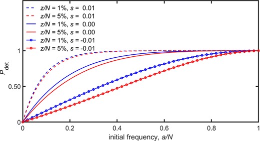
The probability of a detectable result, $P_{det}$ ⁠, is plotted against the initial frequency, $a / N$ ⁠, for the Wright–Fisher model described in the text. The values of $P_{det}$ were calculated from equation (16). For the figure the following parameter values were adopted: population size $N = 500$ ⁠, equal forward and backward mutation rates of $μ = ν = 10^{- 5}$ ⁠, observation time $t_{obs} = 200$ ⁠. The two values of the observation threshold used were $z = 5$ and 25, and these were listed in the Figure Legend as $z / N = 1 %$ and $5 %$ ⁠, respectively.

Open in new tab Download slide

From figure 2, it can be seen that increasing the value of the threshold, z, causes a decrease in the value of $P_{det}$ ⁠, as is understandable since then a decreased proportion of trajectories lie above threshold at the observation time. Furthermore, parameter values which tend to increase the value of $M (t_{obs})$ also tend to increase the value of $P_{det}$ ⁠, thus $P_{det}$ is plausibly an increasing function of both the initial frequency, $a / N$ ⁠, and the selection coefficient, s.

We can also derive expressions, in terms of the transition matrix,

W

⁠, for the expected values of powers of

X (t_{obs}) = M (t_{obs}) / N

⁠. To simplify the notation, we write the unconditional expected value

E {[M (t_{obs}) / N]^{k} | M (0) = a}

simply as

E {[X (t_{obs})]^{k}}

⁠, and the conditional expected value

E {[M (t_{obs}) / N]^{k} | M (0) = a, M (t_{obs}) > z}

simply as

E_{z} {[X (t_{obs})]^{k}}

⁠. We then have, for

k = 1

and

k = 2

⁠:

\begin{aligned} E [X (t_{obs})] = & \sum_{m = 0}^{N} \frac{m}{N} [W^{t_{obs}}]_{m, a} \\ E_{z} [X (t_{obs})] = & \frac{\sum_{m = z + 1}^{N} \frac{m}{N} [W^{t_{obs}}]_{m, a}}{P_{det}} \\ E {[X (t_{obs})]^{2}} = & \sum_{m = 0}^{N} {(\frac{m}{N})}^{2} [W^{t_{obs}}]_{m, a} \\ E_{z} {[X (t_{obs})]^{2}} = & \frac{\sum_{m = z + 1}^{N} {(\frac{m}{N})}^{2} [W^{t_{obs}}]_{m, a}}{P_{det}} \end{aligned}

(17)

with

P_{det}

given in equation (16).

In figure 3, we plot the unconditioned and conditioned expected values of $X (t_{obs})$ ⁠, $[X (t_{obs})]^{2}$ and the associated variances, against the initial frequency, $a / N$ ⁠, for a single observation threshold, z, and different selection coefficients, s.

Fig. 3.

In Panel A the unconditional and conditional expected values of the frequency, namely $E [X (t_{obs})]$ and $E_{z} [X (t_{obs})]$ ⁠, respectively, are plotted against the initial frequency, $a / N$ ⁠, for the Wright–Fisher model described in this work. The expected values were calculated from equation (17). The following parameter values were adopted: population size $N = 500$ ⁠, equal forward and backward mutation rates: $μ = ν = 10^{- 5}$ ⁠, observation time $t_{obs} = 200$ ⁠, and observation threshold $z = 5$ (hence $z / N = 1 %$ ⁠). In Panel B the corresponding unconditional and conditional expected squared values of the frequency, namely $E {[X (t_{obs})]^{2}}$ and $E_{z} {[X (t_{obs})]^{2}}$ ⁠, respectively, are plotted against the initial frequency, $a / N$ ⁠. In Panel C the corresponding variances, namely $Var [X (t_{obs})] = E {[X (t_{obs})]^{2}} - E [X (t_{obs})]^{2}$ and ${Var}_{z} [X (t_{obs})] = E_{z} {[X (t_{obs})]^{2}} - E_{z} [X (t_{obs})]^{2}$ ⁠, are plotted against the initial frequency, $a / N$ ⁠.

Open in new tab Download slide

Figures 3A and 3B illustrate the significant differences that can occur between unconditional and conditional expected values of $X (t_{obs})$ and $[X (t_{obs})]^{2}$ ⁠. As an illustrative example, for the neutral case $(s = 0)$ ⁠, an initial frequency of $a / N = 0.05$ leads to the conditioned expected value of $X (t_{obs})$ being approximately four times the unconditioned value. By contrast the variance of $X (t_{obs})$ ⁠, when calculated using unconditioned and conditioned expected values and plotted in figure 3C, are much closer (note that the vertical scale of Panel C is much smaller than that of Panels A and B), indicating that the moments of $X (t_{obs})$ are more strongly affected by a threshold than the variance.

In figure 4 we illustrate the working of the equality/inequality of equations (8) and (9), the latter for the special case $k = 2$ ⁠. In the notation of the present section, these equations take the form $E [X (t_{obs})] \geq E_{est} [X (t_{obs})] = E_{z} [X (t_{obs})] \times P_{det}$ and $E {[X (t_{obs})]^{2}} \geq E_{est} {[X (t_{obs})]^{2}} =$ $E_{z} {[X (t_{obs})]^{2}} \times P_{det}$ ⁠, respectively.

In Panel A, we plot the unconditional expected value E[X(tobs)] and the quantity Eest[X(tobs)]=Ez[X(tobs)]×Pdet against the initial frequency, a/N. In the Figure Legend, we refer to E[X(tobs)] as “unconditioned” and Eest[X(tobs)] as “estimated.” The probability of a detectable result, Pdet, was calculated from equation (16), while the unconditional and conditional expected values of X(tobs), namely E[X(tobs)] and Ez[X(tobs)], respectively, were calculated from equation (17). For the figure the following parameter values were adopted: population size N=500, forward mutation rate μ=10−5, backward mutation rate ν=10−5, observation time tobs=200, observation threshold z=5 (hence z/N=1%).

Fig. 4.

In Panel A, we plot the unconditional expected value $E [X (t_{obs})]$ and the quantity $E_{est} [X (t_{obs})] = E_{z} [X (t_{obs})] \times P_{det}$ against the initial frequency, $a / N$ ⁠. In the Figure Legend, we refer to $E [X (t_{obs})]$ as “unconditioned” and $E_{est} [X (t_{obs})]$ as “estimated.” The probability of a detectable result, $P_{det}$ ⁠, was calculated from equation (16), while the unconditional and conditional expected values of $X (t_{obs})$ ⁠, namely $E [X (t_{obs})]$ and $E_{z} [X (t_{obs})]$ ⁠, respectively, were calculated from equation (17). For the figure the following parameter values were adopted: population size $N = 500$ ⁠, forward mutation rate $μ = 10^{- 5}$ ⁠, backward mutation rate $ν = 10^{- 5}$ ⁠, observation time $t_{obs} = 200$ ⁠, observation threshold $z = 5$ (hence $z / N = 1 %$ ⁠).

Open in new tab Download slide

In Panel B we give the corresponding plots for $E {[X (t_{obs})]^{2}}$ and $E_{est} {[X (t_{obs})]^{2}} = E_{z} {[X (t_{obs})]^{2}} \times P_{det}$ ⁠, against the initial frequency, $a / N$ ⁠, for the same parameter values.

Figure 4 contains the quantities $E_{est} [X (t_{obs})]$ and $E_{est} {[X (t_{obs})]^{2}}$ ⁠, whose values follow from $E_{z} [X (t_{obs})]$ ⁠, $E_{z} {[X (t_{obs})]^{2}}$ ⁠, and $P_{det}$ ⁠, and hence can be estimated from observations with a threshold operating. The results of figure 4 suggest that $E_{est} [X (t_{obs})]$ and $E_{est} {[X (t_{obs})]^{2}}$ can be used as estimates of the corresponding unconditioned expected values. To explore this over a range of parameters, we have defined four additional statistics, which provide a measure of the mismatch between the “estimates” and the exact unconditioned expected values, as follows.

The first of these new statistics is $R_{max}^{(1)}$ which is the maximum percentage error between the estimated mean frequency, $E_{est} [X (t_{obs})]$ ⁠, and the exact mean frequency, $E [X (t_{obs})]$ ⁠. This statistic is determined by considering all possible initial frequencies, $a / N$ ⁠, and then reporting the largest percentage error between the estimated and exact mean values of the frequency, that is, $R_{max}^{(1)} = max_{a} {1 - E_{est} [X (t_{obs})] / E [X (t_{obs})]} \times 100$ ⁠. Closely related to $R_{max}^{(1)}$ is the statistic $R_{max}^{(2)}$ ⁠, which determines the largest percentage error between the estimated and exact values of the mean square frequency.

Another statistic we introduce is

R_{avg}^{(1)}

which gives the percentage error between the estimated and exact mean values of the frequency, when the error in the mean frequency, when averaged over all possible initial frequencies, that is,

R_{avg}^{(1)} = {mean}_{a} (1 - E_{est} [X (t_{obs})] / E [X (t_{obs})]) \times 100

⁠. Closely related to this is

R_{avg}^{(2)}

⁠, which is the error in the mean square frequency, when averaged over all possible initial frequencies. These new statistics are given in equation (18) and in table 2 we give the values of these statistics for various parameter values.

\begin{matrix} R_{max}^{(1)} & = & max_{a} (1 - \frac{E_{est} [X (t_{obs})]}{E [X (t_{obs})]}) \times 100 \\ R_{avg}^{(1)} & = & {mean}_{a} (1 - \frac{E_{est} [X (t_{obs})]}{E [X (t_{obs})]}) \times 100 \\ R_{max}^{(2)} & = & max_{a} (1 - \frac{E_{est} {[X (t_{obs})]^{2}}}{E {[X (t_{obs})]^{2}}}) \times 100 \\ R_{avg}^{(2)} & = & {mean}_{a} (1 - \frac{E_{est} {[X (t_{obs})]^{2}}}{E {[X (t_{obs})]^{2}}}) \times 100. \end{matrix}

(18)

Table 2.

Open in new tab

Four Sub-tables, Containing Values of the Values of the Quantities $R_{max}^{(1)}$ ⁠, $R_{avg}^{(1)}$ ⁠, $R_{max}^{(2)}$ ⁠, and $R_{avg}^{(2)}$ Defined in equation (18)

(A) $μ = 10^{- 8}$
$t_{obs}$	s	% Error $R_{\max}^{(1)}$	% Error $R_{avg}^{(1)}$
20	−0.01	2.2	0.1
	0.00	1.8	0.1
	0.01	1.5	0.1
50	−0.01	0.6	0.1
	0.00	0.4	<0.1
	0.01	0.2	<0.1
200	−0.01	0.1	<0.1
	0.00	<0.1	<0.1
	0.01	<0.1	<0.1
1,000	−0.01	<0.1	<0.1
	0.00	<0.1	<0.1
	0.01	<0.1	<0.1
20	−0.01	8.0	0.2
	0.00	6.5	0.2
	0.01	5.3	0.1
50	−0.01	2.6	0.2
	0.00	1.6	0.1
	0.01	1.0	<0.1
200	−0.01	0.6	0.2
	0.00	0.1	<0.1
	0.01	<0.1	<0.1
1,000	−0.01	1.0	0.1
	0.00	<0.1	<0.1
	0.01	<0.1	<0.1
20	−0.01	17.1	0.3
	0.00	13.7	0.2
	0.01	10.8	0.1
50	−0.01	7.4	0.3
	0.00	4.6	0.1
	0.01	2.7	0.1
200	−0.01	2.2	0.5
	0.00	0.5	<0.1
	0.01	0.1	<0.1
1,000	−0.01	8.9	1.2
	0.00	<0.1	<0.1
	0.01	<0.1	<0.1

(A) $μ = 10^{- 8}$
$t_{obs}$	s	% Error $R_{\max}^{(1)}$	% Error $R_{avg}^{(1)}$
20	−0.01	2.2	0.1
	0.00	1.8	0.1
	0.01	1.5	0.1
50	−0.01	0.6	0.1
	0.00	0.4	<0.1
	0.01	0.2	<0.1
200	−0.01	0.1	<0.1
	0.00	<0.1	<0.1
	0.01	<0.1	<0.1
1,000	−0.01	<0.1	<0.1
	0.00	<0.1	<0.1
	0.01	<0.1	<0.1
20	−0.01	8.0	0.2
	0.00	6.5	0.2
	0.01	5.3	0.1
50	−0.01	2.6	0.2
	0.00	1.6	0.1
	0.01	1.0	<0.1
200	−0.01	0.6	0.2
	0.00	0.1	<0.1
	0.01	<0.1	<0.1
1,000	−0.01	1.0	0.1
	0.00	<0.1	<0.1
	0.01	<0.1	<0.1
20	−0.01	17.1	0.3
	0.00	13.7	0.2
	0.01	10.8	0.1
50	−0.01	7.4	0.3
	0.00	4.6	0.1
	0.01	2.7	0.1
200	−0.01	2.2	0.5
	0.00	0.5	<0.1
	0.01	0.1	<0.1
1,000	−0.01	8.9	1.2
	0.00	<0.1	<0.1
	0.01	<0.1	<0.1

(B) $μ = 10^{- 5}$
N	$t_{obs}$	s	% Error $R_{\max}^{(1)}$	% Error $R_{avg}^{(1)}$
200	20	−0.01	2.5	0.1
		0.00	2.1	0.1
		0.01	1.7	0.1
	50	−0.01	1.1	0.1
		0.00	0.7	0.1
		0.01	0.4	<0.1
	200	−0.01	1.2	0.1
		0.00	0.4	<0.1
		0.01	0.1	<0.1
	1,000	−0.01	1.6	0.1
		0.00	0.2	<0.1
		0.01	0.1	<0.1
500	20	−0.01	8.3	0.2
		0.00	6.8	0.2
		0.01	5.5	0.1
	50	−0.01	3.5	0.2
		0.00	2.2	0.1
		0.01	1.3	<0.1
	200	−0.01	3.9	0.3
		0.00	0.9	<0.1
		0.01	0.2	<0.1
	1,000	−0.01	8.3	2.6
		0.00	0.5	<0.1
		0.01	0.1	<0.1
1,000	20	−0.01	17.3	0.3
		0.00	13.9	0.2
		0.01	10.9	0.1
	50	−0.01	8.6	0.3
		0.00	5.3	0.1
		0.01	3.1	0.1
	200	−0.01	8.3	0.7
		0.00	1.7	0.1
		0.01	0.3	<0.1
	1,000	−0.01	16.7	10.3
		0.00	0.9	0.1
		0.01	<0.1	<0.1

(B) $μ = 10^{- 5}$
N	$t_{obs}$	s	% Error $R_{\max}^{(1)}$	% Error $R_{avg}^{(1)}$
200	20	−0.01	2.5	0.1
		0.00	2.1	0.1
		0.01	1.7	0.1
	50	−0.01	1.1	0.1
		0.00	0.7	0.1
		0.01	0.4	<0.1
	200	−0.01	1.2	0.1
		0.00	0.4	<0.1
		0.01	0.1	<0.1
	1,000	−0.01	1.6	0.1
		0.00	0.2	<0.1
		0.01	0.1	<0.1
500	20	−0.01	8.3	0.2
		0.00	6.8	0.2
		0.01	5.5	0.1
	50	−0.01	3.5	0.2
		0.00	2.2	0.1
		0.01	1.3	<0.1
	200	−0.01	3.9	0.3
		0.00	0.9	<0.1
		0.01	0.2	<0.1
	1,000	−0.01	8.3	2.6
		0.00	0.5	<0.1
		0.01	0.1	<0.1
1,000	20	−0.01	17.3	0.3
		0.00	13.9	0.2
		0.01	10.9	0.1
	50	−0.01	8.6	0.3
		0.00	5.3	0.1
		0.01	3.1	0.1
	200	−0.01	8.3	0.7
		0.00	1.7	0.1
		0.01	0.3	<0.1
	1,000	−0.01	16.7	10.3
		0.00	0.9	0.1
		0.01	<0.1	<0.1

(C) $μ = 10^{- 8}$
$t_{obs}$	s	% Error $R_{\max}^{(2)}$	% Error $R_{avg}^{(2)}$
20	−0.01	0.2	<0.1
	0.00	0.1	<0.1
	0.01	0.1	<0.1
50	−0.01	<0.1	<0.1
	0.00	<0.1	<0.1
	0.01	<0.1	<0.1
200	−0.01	<0.1	<0.1
	0.00	<0.1	<0.1
	0.01	<0.1	<0.1
1,000	−0.01	<0.1	<0.1
	0.00	<0.1	<0.1
	0.01	<0.1	<0.1
20	−0.01	1.3	<0.1
	0.00	1.0	<0.1
	0.01	0.7	<0.1
50	−0.01	0.2	<0.1
	0.00	0.1	<0.1
	0.01	0.1	<0.1
200	−0.01	<0.1	<0.1
	0.00	<0.1	<0.1
	0.01	<0.1	<0.1
1,000	−0.01	<0.1	<0.1
	0.00	<0.1	<0.1
	0.01	<0.1	<0.1
20	−0.01	4.4	0.1
	0.00	3.1	<0.1
	0.01	2.2	<0.1
50	−0.01	1.1	<0.1
	0.00	0.5	<0.1
	0.01	0.2	<0.1
200	−0.01	0.2	<0.1
	0.00	<0.1	<0.1
	0.01	<0.1	<0.1
1,000	−0.01	0.6	0.1
	0.00	<0.1	<0.1
	0.01	<0.1	<0.1

(C) $μ = 10^{- 8}$
$t_{obs}$	s	% Error $R_{\max}^{(2)}$	% Error $R_{avg}^{(2)}$
20	−0.01	0.2	<0.1
	0.00	0.1	<0.1
	0.01	0.1	<0.1
50	−0.01	<0.1	<0.1
	0.00	<0.1	<0.1
	0.01	<0.1	<0.1
200	−0.01	<0.1	<0.1
	0.00	<0.1	<0.1
	0.01	<0.1	<0.1
1,000	−0.01	<0.1	<0.1
	0.00	<0.1	<0.1
	0.01	<0.1	<0.1
20	−0.01	1.3	<0.1
	0.00	1.0	<0.1
	0.01	0.7	<0.1
50	−0.01	0.2	<0.1
	0.00	0.1	<0.1
	0.01	0.1	<0.1
200	−0.01	<0.1	<0.1
	0.00	<0.1	<0.1
	0.01	<0.1	<0.1
1,000	−0.01	<0.1	<0.1
	0.00	<0.1	<0.1
	0.01	<0.1	<0.1
20	−0.01	4.4	0.1
	0.00	3.1	<0.1
	0.01	2.2	<0.1
50	−0.01	1.1	<0.1
	0.00	0.5	<0.1
	0.01	0.2	<0.1
200	−0.01	0.2	<0.1
	0.00	<0.1	<0.1
	0.01	<0.1	<0.1
1,000	−0.01	0.6	0.1
	0.00	<0.1	<0.1
	0.01	<0.1	<0.1

(D) $μ = 10^{- 5}$
N	$t_{obs}$	s	% Error $R_{\max}^{(2)}$	% Error $R_{avg}^{(2)}$
200	20	−0.01	0.2	<0.1
		0.00	0.2	<0.1
		0.01	0.1	<0.1
	50	−0.01	<0.1	<0.1
		0.00	<0.1	<0.1
		0.01	<0.1	<0.1
	200	−0.01	<0.1	<0.1
		0.00	<0.1	<0.1
		0.01	<0.1	<0.1
	1,000	−0.01	<0.1	<0.1
		0.00	<0.1	<0.1
		0.01	<0.1	<0.1
500	20	−0.01	1.3	<0.1
		0.00	1.0	<0.1
		0.01	0.7	<0.1
	50	−0.01	0.3	<0.1
		0.00	0.1	<0.1
		0.01	0.1	<0.1
	200	−0.01	0.2	<0.1
		0.00	<0.1	<0.1
		0.01	<0.1	<0.1
	1,000	−0.01	0.4	<0.1
		0.00	<0.1	<0.1
		0.01	<0.1	<0.1
1,000	20	−0.01	4.4	0.1
		0.00	3.1	<0.1
		0.01	2.2	<0.1
	50	−0.01	1.3	<0.1
		0.00	0.6	<0.1
		0.01	0.3	<0.1
	200	−0.01	0.6	<0.1
		0.00	0.1	<0.1
		0.01	<0.1	<0.1
	1,000	−0.01	1.6	0.8
		0.00	<0.1	<0.1
		0.01	<0.1	<0.1

(D) $μ = 10^{- 5}$
N	$t_{obs}$	s	% Error $R_{\max}^{(2)}$	% Error $R_{avg}^{(2)}$
200	20	−0.01	0.2	<0.1
		0.00	0.2	<0.1
		0.01	0.1	<0.1
	50	−0.01	<0.1	<0.1
		0.00	<0.1	<0.1
		0.01	<0.1	<0.1
	200	−0.01	<0.1	<0.1
		0.00	<0.1	<0.1
		0.01	<0.1	<0.1
	1,000	−0.01	<0.1	<0.1
		0.00	<0.1	<0.1
		0.01	<0.1	<0.1
500	20	−0.01	1.3	<0.1
		0.00	1.0	<0.1
		0.01	0.7	<0.1
	50	−0.01	0.3	<0.1
		0.00	0.1	<0.1
		0.01	0.1	<0.1
	200	−0.01	0.2	<0.1
		0.00	<0.1	<0.1
		0.01	<0.1	<0.1
	1,000	−0.01	0.4	<0.1
		0.00	<0.1	<0.1
		0.01	<0.1	<0.1
1,000	20	−0.01	4.4	0.1
		0.00	3.1	<0.1
		0.01	2.2	<0.1
	50	−0.01	1.3	<0.1
		0.00	0.6	<0.1
		0.01	0.3	<0.1
	200	−0.01	0.6	<0.1
		0.00	0.1	<0.1
		0.01	<0.1	<0.1
	1,000	−0.01	1.6	0.8
		0.00	<0.1	<0.1
		0.01	<0.1	<0.1

Note:—The quantity $R_{max}^{(1)}$ is the maximum percentage difference between $E [X (t_{obs})]$ and $E_{est} [X (t_{obs})] = E_{z} [X (t_{obs})] \times P_{det}$ ⁠, while $R_{avg}^{(1)}$ is the mean percentage difference of these quantities, with corresponding interpretations of $R_{max}^{(2)}$ and $R_{avg}^{(2)}$ ⁠, for the squared frequencies. In all sub-tables, an observation threshold corresponding to $z / N = 1 %$ was adopted. In all sub-tables, equal forward and backward mutation rates were adopted; in sub-tables 2A and 2C we took $μ = ν = 10^{- 8}$ ⁠, while in sub-tables 2B and 2D we took $μ = ν = 10^{- 5}$ ⁠.

Table 2.

Open in new tab

Four Sub-tables, Containing Values of the Values of the Quantities $R_{max}^{(1)}$ ⁠, $R_{avg}^{(1)}$ ⁠, $R_{max}^{(2)}$ ⁠, and $R_{avg}^{(2)}$ Defined in equation (18)

(A) $μ = 10^{- 8}$
$t_{obs}$	s	% Error $R_{\max}^{(1)}$	% Error $R_{avg}^{(1)}$
20	−0.01	2.2	0.1
	0.00	1.8	0.1
	0.01	1.5	0.1
50	−0.01	0.6	0.1
	0.00	0.4	<0.1
	0.01	0.2	<0.1
200	−0.01	0.1	<0.1
	0.00	<0.1	<0.1
	0.01	<0.1	<0.1
1,000	−0.01	<0.1	<0.1
	0.00	<0.1	<0.1
	0.01	<0.1	<0.1
20	−0.01	8.0	0.2
	0.00	6.5	0.2
	0.01	5.3	0.1
50	−0.01	2.6	0.2
	0.00	1.6	0.1
	0.01	1.0	<0.1
200	−0.01	0.6	0.2
	0.00	0.1	<0.1
	0.01	<0.1	<0.1
1,000	−0.01	1.0	0.1
	0.00	<0.1	<0.1
	0.01	<0.1	<0.1
20	−0.01	17.1	0.3
	0.00	13.7	0.2
	0.01	10.8	0.1
50	−0.01	7.4	0.3
	0.00	4.6	0.1
	0.01	2.7	0.1
200	−0.01	2.2	0.5
	0.00	0.5	<0.1
	0.01	0.1	<0.1
1,000	−0.01	8.9	1.2
	0.00	<0.1	<0.1
	0.01	<0.1	<0.1

(A) $μ = 10^{- 8}$
$t_{obs}$	s	% Error $R_{\max}^{(1)}$	% Error $R_{avg}^{(1)}$
20	−0.01	2.2	0.1
	0.00	1.8	0.1
	0.01	1.5	0.1
50	−0.01	0.6	0.1
	0.00	0.4	<0.1
	0.01	0.2	<0.1
200	−0.01	0.1	<0.1
	0.00	<0.1	<0.1
	0.01	<0.1	<0.1
1,000	−0.01	<0.1	<0.1
	0.00	<0.1	<0.1
	0.01	<0.1	<0.1
20	−0.01	8.0	0.2
	0.00	6.5	0.2
	0.01	5.3	0.1
50	−0.01	2.6	0.2
	0.00	1.6	0.1
	0.01	1.0	<0.1
200	−0.01	0.6	0.2
	0.00	0.1	<0.1
	0.01	<0.1	<0.1
1,000	−0.01	1.0	0.1
	0.00	<0.1	<0.1
	0.01	<0.1	<0.1
20	−0.01	17.1	0.3
	0.00	13.7	0.2
	0.01	10.8	0.1
50	−0.01	7.4	0.3
	0.00	4.6	0.1
	0.01	2.7	0.1
200	−0.01	2.2	0.5
	0.00	0.5	<0.1
	0.01	0.1	<0.1
1,000	−0.01	8.9	1.2
	0.00	<0.1	<0.1
	0.01	<0.1	<0.1

(B) $μ = 10^{- 5}$
N	$t_{obs}$	s	% Error $R_{\max}^{(1)}$	% Error $R_{avg}^{(1)}$
200	20	−0.01	2.5	0.1
		0.00	2.1	0.1
		0.01	1.7	0.1
	50	−0.01	1.1	0.1
		0.00	0.7	0.1
		0.01	0.4	<0.1
	200	−0.01	1.2	0.1
		0.00	0.4	<0.1
		0.01	0.1	<0.1
	1,000	−0.01	1.6	0.1
		0.00	0.2	<0.1
		0.01	0.1	<0.1
500	20	−0.01	8.3	0.2
		0.00	6.8	0.2
		0.01	5.5	0.1
	50	−0.01	3.5	0.2
		0.00	2.2	0.1
		0.01	1.3	<0.1
	200	−0.01	3.9	0.3
		0.00	0.9	<0.1
		0.01	0.2	<0.1
	1,000	−0.01	8.3	2.6
		0.00	0.5	<0.1
		0.01	0.1	<0.1
1,000	20	−0.01	17.3	0.3
		0.00	13.9	0.2
		0.01	10.9	0.1
	50	−0.01	8.6	0.3
		0.00	5.3	0.1
		0.01	3.1	0.1
	200	−0.01	8.3	0.7
		0.00	1.7	0.1
		0.01	0.3	<0.1
	1,000	−0.01	16.7	10.3
		0.00	0.9	0.1
		0.01	<0.1	<0.1

(B) $μ = 10^{- 5}$
N	$t_{obs}$	s	% Error $R_{\max}^{(1)}$	% Error $R_{avg}^{(1)}$
200	20	−0.01	2.5	0.1
		0.00	2.1	0.1
		0.01	1.7	0.1
	50	−0.01	1.1	0.1
		0.00	0.7	0.1
		0.01	0.4	<0.1
	200	−0.01	1.2	0.1
		0.00	0.4	<0.1
		0.01	0.1	<0.1
	1,000	−0.01	1.6	0.1
		0.00	0.2	<0.1
		0.01	0.1	<0.1
500	20	−0.01	8.3	0.2
		0.00	6.8	0.2
		0.01	5.5	0.1
	50	−0.01	3.5	0.2
		0.00	2.2	0.1
		0.01	1.3	<0.1
	200	−0.01	3.9	0.3
		0.00	0.9	<0.1
		0.01	0.2	<0.1
	1,000	−0.01	8.3	2.6
		0.00	0.5	<0.1
		0.01	0.1	<0.1
1,000	20	−0.01	17.3	0.3
		0.00	13.9	0.2
		0.01	10.9	0.1
	50	−0.01	8.6	0.3
		0.00	5.3	0.1
		0.01	3.1	0.1
	200	−0.01	8.3	0.7
		0.00	1.7	0.1
		0.01	0.3	<0.1
	1,000	−0.01	16.7	10.3
		0.00	0.9	0.1
		0.01	<0.1	<0.1

(C) $μ = 10^{- 8}$
$t_{obs}$	s	% Error $R_{\max}^{(2)}$	% Error $R_{avg}^{(2)}$
20	−0.01	0.2	<0.1
	0.00	0.1	<0.1
	0.01	0.1	<0.1
50	−0.01	<0.1	<0.1
	0.00	<0.1	<0.1
	0.01	<0.1	<0.1
200	−0.01	<0.1	<0.1
	0.00	<0.1	<0.1
	0.01	<0.1	<0.1
1,000	−0.01	<0.1	<0.1
	0.00	<0.1	<0.1
	0.01	<0.1	<0.1
20	−0.01	1.3	<0.1
	0.00	1.0	<0.1
	0.01	0.7	<0.1
50	−0.01	0.2	<0.1
	0.00	0.1	<0.1
	0.01	0.1	<0.1
200	−0.01	<0.1	<0.1
	0.00	<0.1	<0.1
	0.01	<0.1	<0.1
1,000	−0.01	<0.1	<0.1
	0.00	<0.1	<0.1
	0.01	<0.1	<0.1
20	−0.01	4.4	0.1
	0.00	3.1	<0.1
	0.01	2.2	<0.1
50	−0.01	1.1	<0.1
	0.00	0.5	<0.1
	0.01	0.2	<0.1
200	−0.01	0.2	<0.1
	0.00	<0.1	<0.1
	0.01	<0.1	<0.1
1,000	−0.01	0.6	0.1
	0.00	<0.1	<0.1
	0.01	<0.1	<0.1

(C) $μ = 10^{- 8}$
$t_{obs}$	s	% Error $R_{\max}^{(2)}$	% Error $R_{avg}^{(2)}$
20	−0.01	0.2	<0.1
	0.00	0.1	<0.1
	0.01	0.1	<0.1
50	−0.01	<0.1	<0.1
	0.00	<0.1	<0.1
	0.01	<0.1	<0.1
200	−0.01	<0.1	<0.1
	0.00	<0.1	<0.1
	0.01	<0.1	<0.1
1,000	−0.01	<0.1	<0.1
	0.00	<0.1	<0.1
	0.01	<0.1	<0.1
20	−0.01	1.3	<0.1
	0.00	1.0	<0.1
	0.01	0.7	<0.1
50	−0.01	0.2	<0.1
	0.00	0.1	<0.1
	0.01	0.1	<0.1
200	−0.01	<0.1	<0.1
	0.00	<0.1	<0.1
	0.01	<0.1	<0.1
1,000	−0.01	<0.1	<0.1
	0.00	<0.1	<0.1
	0.01	<0.1	<0.1
20	−0.01	4.4	0.1
	0.00	3.1	<0.1
	0.01	2.2	<0.1
50	−0.01	1.1	<0.1
	0.00	0.5	<0.1
	0.01	0.2	<0.1
200	−0.01	0.2	<0.1
	0.00	<0.1	<0.1
	0.01	<0.1	<0.1
1,000	−0.01	0.6	0.1
	0.00	<0.1	<0.1
	0.01	<0.1	<0.1

(D) $μ = 10^{- 5}$
N	$t_{obs}$	s	% Error $R_{\max}^{(2)}$	% Error $R_{avg}^{(2)}$
200	20	−0.01	0.2	<0.1
		0.00	0.2	<0.1
		0.01	0.1	<0.1
	50	−0.01	<0.1	<0.1
		0.00	<0.1	<0.1
		0.01	<0.1	<0.1
	200	−0.01	<0.1	<0.1
		0.00	<0.1	<0.1
		0.01	<0.1	<0.1
	1,000	−0.01	<0.1	<0.1
		0.00	<0.1	<0.1
		0.01	<0.1	<0.1
500	20	−0.01	1.3	<0.1
		0.00	1.0	<0.1
		0.01	0.7	<0.1
	50	−0.01	0.3	<0.1
		0.00	0.1	<0.1
		0.01	0.1	<0.1
	200	−0.01	0.2	<0.1
		0.00	<0.1	<0.1
		0.01	<0.1	<0.1
	1,000	−0.01	0.4	<0.1
		0.00	<0.1	<0.1
		0.01	<0.1	<0.1
1,000	20	−0.01	4.4	0.1
		0.00	3.1	<0.1
		0.01	2.2	<0.1
	50	−0.01	1.3	<0.1
		0.00	0.6	<0.1
		0.01	0.3	<0.1
	200	−0.01	0.6	<0.1
		0.00	0.1	<0.1
		0.01	<0.1	<0.1
	1,000	−0.01	1.6	0.8
		0.00	<0.1	<0.1
		0.01	<0.1	<0.1

(D) $μ = 10^{- 5}$
N	$t_{obs}$	s	% Error $R_{\max}^{(2)}$	% Error $R_{avg}^{(2)}$
200	20	−0.01	0.2	<0.1
		0.00	0.2	<0.1
		0.01	0.1	<0.1
	50	−0.01	<0.1	<0.1
		0.00	<0.1	<0.1
		0.01	<0.1	<0.1
	200	−0.01	<0.1	<0.1
		0.00	<0.1	<0.1
		0.01	<0.1	<0.1
	1,000	−0.01	<0.1	<0.1
		0.00	<0.1	<0.1
		0.01	<0.1	<0.1
500	20	−0.01	1.3	<0.1
		0.00	1.0	<0.1
		0.01	0.7	<0.1
	50	−0.01	0.3	<0.1
		0.00	0.1	<0.1
		0.01	0.1	<0.1
	200	−0.01	0.2	<0.1
		0.00	<0.1	<0.1
		0.01	<0.1	<0.1
	1,000	−0.01	0.4	<0.1
		0.00	<0.1	<0.1
		0.01	<0.1	<0.1
1,000	20	−0.01	4.4	0.1
		0.00	3.1	<0.1
		0.01	2.2	<0.1
	50	−0.01	1.3	<0.1
		0.00	0.6	<0.1
		0.01	0.3	<0.1
	200	−0.01	0.6	<0.1
		0.00	0.1	<0.1
		0.01	<0.1	<0.1
	1,000	−0.01	1.6	0.8
		0.00	<0.1	<0.1
		0.01	<0.1	<0.1

In table 2 we have explored how the error statistics we have introduced (namely $R_{max}^{(1)}$ ⁠, $R_{avg}^{(1)}$ ⁠, $R_{max}^{(2)}$ and $R_{avg}^{(2)}$ ⁠) behave for different values of the parameters N, $t_{obs}$ ⁠, s, and $μ$ (⁠ $= ν$ ⁠). Generally, table 2 indicates that the errors between the actual and estimated values of: (i) $E [X (t_{obs})]$ ⁠, and (ii) $E {[X (t_{obs})]^{2}}$ ⁠, are very reasonable. The single parameter that has the largest effect on the quality of the approximations is the observation time $t_{obs}$ ⁠. Small values of $t_{obs}$ appear to yield the largest errors in the estimated. For example, in table 2A, a value of $t_{obs}$ of 20 generations can lead to an error of approximately $17 %$ in the approximation of $E [X (t_{obs})]$ ⁠, while larger values of $t_{obs}$ lead to smaller (often substantially smaller) errors. There appears to be no great sensitivity of the error statistics on N, s, and $μ$ ⁠.

Discussion

In this work, we have shown that observation thresholds may severely bias estimates of allele frequencies. The results presented can be directly applied to a set of mutations which are present or which are de-novo mutations at initial frequency $1 / N$ or $1 / (2 N)$ ⁠, for haploid or diploid populations, respectively. Most importantly, our approach would also apply to scenarios where we assume a large number of sites in the genome that, at $t = 0$ ⁠, have different frequencies of for example, a minor allele, and then we inspect the allele frequencies some time later. This arises because if we follow trajectories whose initial frequencies are distributed according to an arbitrary initial distribution, then some will not be detected at the time-point $t_{obs}$ —due to being below threshold. However, the expected value of for example, $X (t_{obs})$ ⁠, that would follow from all trajectories, if no threshold at $t_{obs}$ existed, can be retrieved from the expected value that is calculated only from the detected trajectories, when multiplied with $P_{det}$ ⁠. An example of the values of $P_{det}$ ⁠, based on data from six different Drosophila melanogaster populations (Kapun et al. 2021) is given in table 3. Note, that we do not consider varying levels of the threshold here, but determine the extent of it, assuming a constant threshold for each sample. For this we neglect mutations that arise de-novo or that get truly fixed between the two timepoints, as these will be extremely rare. Also, ideally we would expect that there is no threshold at timepoint 1, which is however unrealistic for this dataset. Hence, we also neglect those mutations that segregate below threshold at timepoint 1 (as these cannot be measured). We would expect that those mutations below threshold at timepoint 1 are more likely to segregate below threshold at timepoint 2 relative to the observed trajectories at time point 1. Hence our derived $P_{det}$ can be considered an overestimate of the true $P_{det}$ ⁠. Under these assumptions the values of $P_{det}$ ⁠, that are estimated from the data, range from $0.58$ to $0.84$ suggesting that an observation bias is operating, with non-negligible effect, that is particularly significant for variants segregating at low frequencies.

Table 3.

Open in new tab

Magnitude of $P_{det}$ Estimated for Six Different Drosophila melanogaster Populations Obtained from Pooled Genome Sequencing at Two Different Time Points (Kapun et al. 2021)

Sample Timepoint 1	Sample Timepoint 2	Minor SNP Frequency at Timepoint 1	Number of Observed SNPs at Timepoint 1	Number of SNPs Observed at Timepoint 1 and Timepoint 2	P_det
AT_See_14_44	AT_See_16_1	Any	527,942	420,466	79.64%
		<10%	240,580	152,708	63.47%
ES_Gim_14_35	ES_Gim_14_34	Any	500,999	389,344	77.71%
		<10%	212,550	123,828	58.26%
MA_la_14_spring	MA_la_14_fall	Any	566,427	493,377	87.10%
		<10%	285,214	224,694	78.78%
FI_Aka_14_36	FI_Aka_14_37	Any	480,143	394,569	82.18%
		<10%	193,899	126,987	65.49%
AT_Mau_14_01	AT_Mau_14_02	Any	501,657	403,311	80.40%
		<10%	239,259	152,665	63.81%
DE_Mun_14_31	DE_Mun_14_32	Any	495,287	414,226	83.63%
		<10%	194,432	131,869	67.82%

Sample Timepoint 1	Sample Timepoint 2	Minor SNP Frequency at Timepoint 1	Number of Observed SNPs at Timepoint 1	Number of SNPs Observed at Timepoint 1 and Timepoint 2	P_det
AT_See_14_44	AT_See_16_1	Any	527,942	420,466	79.64%
		<10%	240,580	152,708	63.47%
ES_Gim_14_35	ES_Gim_14_34	Any	500,999	389,344	77.71%
		<10%	212,550	123,828	58.26%
MA_la_14_spring	MA_la_14_fall	Any	566,427	493,377	87.10%
		<10%	285,214	224,694	78.78%
FI_Aka_14_36	FI_Aka_14_37	Any	480,143	394,569	82.18%
		<10%	193,899	126,987	65.49%
AT_Mau_14_01	AT_Mau_14_02	Any	501,657	403,311	80.40%
		<10%	239,259	152,665	63.81%
DE_Mun_14_31	DE_Mun_14_32	Any	495,287	414,226	83.63%
		<10%	194,432	131,869	67.82%

Note.—The number of single nucleotide polymophisms (SNPs) at timepoint 1, and the number of SNPs at timepoint 2 that are also observed at timepoint 1 are shown. For simplicity, only biallelic SNPs on chromosome arm 2L are considered.

Table 3.

Open in new tab

Magnitude of $P_{det}$ Estimated for Six Different Drosophila melanogaster Populations Obtained from Pooled Genome Sequencing at Two Different Time Points (Kapun et al. 2021)

Sample Timepoint 1	Sample Timepoint 2	Minor SNP Frequency at Timepoint 1	Number of Observed SNPs at Timepoint 1	Number of SNPs Observed at Timepoint 1 and Timepoint 2	P_det
AT_See_14_44	AT_See_16_1	Any	527,942	420,466	79.64%
		<10%	240,580	152,708	63.47%
ES_Gim_14_35	ES_Gim_14_34	Any	500,999	389,344	77.71%
		<10%	212,550	123,828	58.26%
MA_la_14_spring	MA_la_14_fall	Any	566,427	493,377	87.10%
		<10%	285,214	224,694	78.78%
FI_Aka_14_36	FI_Aka_14_37	Any	480,143	394,569	82.18%
		<10%	193,899	126,987	65.49%
AT_Mau_14_01	AT_Mau_14_02	Any	501,657	403,311	80.40%
		<10%	239,259	152,665	63.81%
DE_Mun_14_31	DE_Mun_14_32	Any	495,287	414,226	83.63%
		<10%	194,432	131,869	67.82%

Sample Timepoint 1	Sample Timepoint 2	Minor SNP Frequency at Timepoint 1	Number of Observed SNPs at Timepoint 1	Number of SNPs Observed at Timepoint 1 and Timepoint 2	P_det
AT_See_14_44	AT_See_16_1	Any	527,942	420,466	79.64%
		<10%	240,580	152,708	63.47%
ES_Gim_14_35	ES_Gim_14_34	Any	500,999	389,344	77.71%
		<10%	212,550	123,828	58.26%
MA_la_14_spring	MA_la_14_fall	Any	566,427	493,377	87.10%
		<10%	285,214	224,694	78.78%
FI_Aka_14_36	FI_Aka_14_37	Any	480,143	394,569	82.18%
		<10%	193,899	126,987	65.49%
AT_Mau_14_01	AT_Mau_14_02	Any	501,657	403,311	80.40%
		<10%	239,259	152,665	63.81%
DE_Mun_14_31	DE_Mun_14_32	Any	495,287	414,226	83.63%
		<10%	194,432	131,869	67.82%

We note, that in the example given in table 3 we do not estimate the threshold z, but $P_{\det}$ ⁠, as this can be used as a correction factor. While we use z as a parameter to derive the mathematical underpinnings, we cannot estimate z from relative allele frequency data used here. When there is a correlation between read depth and particular sites, the parameter $P_{\det}$ will likely be different for different sites. In this case, an overall $P_{\det}$ could be interpreted as a summary statistic capturing properties of an effective (implicit) threshold z across sites.

Our model is also directly relevant to other population genetic scenarios, for example cases where there is the same allele frequency at many (potentially neutral) loci, as a consequence (mass) migration events or secondary contacts of separated populations. We emphasize that while the observation threshold is described as a measurement of a single quantity, for example, the frequency of a “new” mutational type, which is of biological relevance when reference-based mapping is applied (e.g., read mapping a reference genome), our model can be extended to more complex scenarios of observational thresholds.

We have posed two basic questions in this work. First, we asked when conditioning, associated with an observation threshold, has a large effect on the observed results. Equation (8), when approximated as an inequality, gives a clear indication of this: the smaller the probability of detecting a result when the population is observed (⁠ $P_{det}$ ⁠), the larger the discrepancy between the unconditioned mean allele frequency (where there is no observation threshold and the measurement is ideal) and the conditioned mean allele frequency (fig. 3). The way $P_{det}$ changes with parameters in the model allows us to give a more nuanced answer to the question. Thus the discrepancy between unconditioned and conditioned mean allele frequencies is most severe when the initial frequency at which the mutation was present or arose in the population is small, but this effect appears more pronounced for larger selection coefficients. For mutations under purifying selection (i.e., with $s < 0$ ⁠) the discrepancy between unconditioned and conditioned expected values of the frequency appears to be relatively substantial even for larger initial frequencies (fig. 3). Generally, we infer that a key measure of the effect of the strength of conditioning is the value of $P_{det}$ ⁠. Most intriguingly, we can show that for low initial frequencies a conditioned measurement may have the same expected frequency as an unconditioned case with a larger selection coefficient (fig. 5). This illustrates that conditioned measurements may lead to a misinference of the underlying selection coefficient.

Fig. 5.

The unconditioned and conditioned expected values of $X (t_{obs})$ (⁠ $E [X (t_{obs})]$ and $E_{z} [X (t_{obs})]$ ⁠, respectively), are plotted against the initial frequency, $a / N$ ⁠, for the Wright–Fisher model described in this work. The expected values were calculated from equation (17), when different selection coefficients were used in the unconditioned and conditioned expected values. The following parameter values were adopted: population size $N = 500$ ⁠, equal forward and backward mutation rates: $μ = ν = 10^{- 5}$ ⁠, observation time $t_{obs} = 200$ ⁠, observation threshold $z = 5$ (hence $z / N = 1 %$ ⁠).

Open in new tab Download slide

A second question we asked, which is of practical significance, concerned the principled way to correct for the effects of the conditioning due to an observational threshold. To address this question, we again used equation (8), which takes the form of an inequality that can be applied to unconditioned and conditioned mean allele frequencies. The inequality provides a lower bound on the value of the unconditioned mean allele frequency. Approximating the inequality by an equality leads to an analytical estimate of the unconditioned mean allele frequency that corrects for bias arising from an observational threshold. Our estimate could, for the scenarios considered in this work, reasonably correct biased estimates of the mean allele frequency, when the mean conditioned allele frequency is known (estimated from measurements), and is combined with knowledge of the probability of detecting a result (also estimated from measurements) (fig. 3). Our numerical results suggest that this correction is reasonably accurate (see table 1) , suggesting that quantifying and incorporating observational thresholds into measurements appears feasible.

Guidelines for Allele Trajectory Data

Our method can be applied to time-series data to determine the possible extent of an observation threshold. As causes of an observation threshold may originate from multiple factors which may not be obvious or cannot be eliminated during measurements, we can apply our method to account for observation bias:

Guideline 1: Assuming that a correction can be applied to the test statistic, that there is some possibility to alter the applied threshold (e.g., through a bioinformatic pipeline) and that there is reasonable concern about false positives at low thresholds, it might be advisable to increase the threshold level and then apply the correction.

Guideline 2: In case a correction cannot be (trivially) applied to the test statistic, but there is still some influence on the threshold, the user may explore different parameter combination on the extent of threshold by determining $P_{det}$ as shown for Kapun et al. (2021) in table 3. It may be advisable to reduce the threshold impact on $P_{det}$ or to homogenize its impact across samples.

Wider Applicability

Lastly, we note that the results we obtain in this work for allele trajectories have wider generality, and apply to many other Markov chains. What they need to have in common, for the results to apply, is that they may be viewed as consisting of either: (i) many statistically equivalent replicates, where observations are made on all replicates at a given time (the observation time), or (ii) many measurements of a stationary system, which are all made at the end of non-overlapping time-intervals of fixed length.

Acknowledgments

We want to thank the anonymous reviewers for their valuable feedback. We acknowledge support for the publication costs by the Open Access Publication Fund of Bielefeld University.

Data Availability

There are no new data associated with this article.

Appendix A: Probability of a Detectable Result and Conditional Distribution

In this appendix, we give details of the determination of the probability of a detectable result.

We work in the context of a discrete state, discrete time Markov chain where $M (t)$ is the state of the system at time t, with $t = 0, 1, 2, \dots, t_{obs}$ and $M (t)$ can take the values $0, 1, 2, \dots, N$ ⁠.

To determine the probability of a detectable result, $P_{det} = Prob [M (t_{obs}) > z]$ we first determine the unconditioned probability distribution of $M (t_{obs})$ ⁠. The distribution of $M (0)$ is assumed known and given by the column vector $Φ (0)$ ⁠, where the m’th element of $Φ (0)$ ⁠, written $Φ_{m} (0)$ (⁠ $m = 0, 1, \dots, N$ ⁠), is the probability that $M (0) = m$ ⁠, that is, $Φ_{m} (0) = Prob [M (0) = m]$ ⁠. The distribution at any time $t > 0$ is given by $Φ (t) = K (t | 0) Φ (0)$ where $K (t | 0)$ is a special case of the matrix $K (t | u)$ introduced in the main text. The $(m, n)$ element of $K (t | 0)$ is the probability that $M (t) = m$ ⁠, given that $M (0) = n$ ⁠, that is, $K_{m, n} (t | 0) = Prob [M (t) = m | M (0) = n]$ ⁠. The probability of an above threshold state at time $t_{obs}$ is given by $P_{det} = \sum_{b = z + 1}^{N} Φ_{b} (t_{obs}) = \sum_{b = z + 1}^{N} \sum_{m = 0}^{N} K_{b, m} (t_{obs} | 0) Φ_{m} (0)$ ⁠. We write this last result as $P_{det} = \sum_{m = 0}^{N} Q_{m} Φ_{m} (0)$ where $Q_{m} = \sum_{b = z + 1}^{N} K_{b, m} (t_{obs} | 0) \equiv \sum_{b > z} K_{b, m} (t_{obs} | 0)$ ⁠. In the special case where only state a occurs at time 0 we have $Φ_{m} (0) = δ_{m, a}$ where $δ_{m, a}$ is a Kronecker delta (⁠ $δ_{m, a}$ is 1 when $m = a$ and is zero otherwise). This leads to $P_{det} = \sum_{m = 0}^{N} Q_{m} δ_{m, a} = Q_{a}$ ⁠.

Appendix B: Conditional Distribution

In this appendix, we give details of the conditional probability distribution, corresponding to the system lying above threshold $(> z)$ at time $t_{obs}$ ⁠.

To determine the probability distribution of

M (t_{obs})

that is conditional on

M (t_{obs}) > z

⁠, we set the conditional distribution to zero if

M (t_{obs}) \leq z

⁠, while if

M (t_{obs}) > z

then the conditional distribution is proportional to the unconditional distribution. Using the Heaviside step function

Θ (m) = {\begin{matrix} 1, & m > 0 \\ 0, & m \leq 0 \end{matrix} (B 1)

(B1)

we thus have, for the conditional distribution,

Φ_{m}^{cond} (t_{obs}) \propto Θ (m - z) Φ_{m} (t_{obs})

⁠. On normalizing this to unity, and using the definition of

P_{det}

(see Appendix A) gives

Φ_{m}^{cond} (t_{obs}) = \frac{Θ (m - z) Φ_{m} (t_{obs})}{\sum_{b = 0}^{N} Θ (b - z) Φ_{b} (t_{obs})} = \frac{Θ (m - z) Φ_{m} (t_{obs})}{P_{det}} . (B 2)

(B2)

Appendix C: Relation between Conditional and Unconditional Values of $M (t_{obs})$

In this appendix, we establish a relation between the expected value of $M (t_{obs}$ ⁠), when conditioned to lie above the threshold value z, and the unconditional expected value of $M (t_{obs})$ ⁠.

For the purposes of this appendix, we shall use the notation M for

M (t_{obs})

and

E [M]

for

E [M (t_{obs})]

⁠, which is the unconditioned expected value of

M (t_{obs})

for an arbitrary initial distribution. The expected value of

M (t_{obs})

when it is conditioned to be

> z

\leq z

is then written as

E [M | M > z]

E [M | M \leq z]

⁠, respectively. We can then write

\begin{aligned} E [M] = & E [M | M > z] \times Prob (M > z) \\ + E [M | M \leq z] \times Prob (M \leq z) . \end{aligned} (C 1)

(C1)

Throughout the paper, we assume that

Prob (M > z) < 1

so that

Prob (M \leq z) = 1 - Prob (M > z) > 0

⁠, and there is a non-zero probability that some states of the system lie below threshold at time

t_{obs}

⁠. This means that if we start with a very large number of trajectories of the system at time 0, the observation threshold will cause a non-zero reduction in the number detected at time

t_{obs}

⁠.

It is instructive to show that conditioning on a threshold generally increases the expected value of M, and the factors which govern this increase. We note the difference between

E [M | M > z]

and

E [M]

is, using equation (C1),

\begin{aligned} E [M | M > z] - E [M] \\ = E [M | M > z] \times [1 - Prob (M > z)] \\ - E [M | M \leq z] \times Prob (M \leq z) \\ = (E [M | M > z] - E [M | M \leq z]) \times [1 - Prob (M > z)] . \end{aligned} (C 2)

(C2)

Because

E [M | M > z] - E [M | M \leq z] > 0

and by assumption

Prob (M > z) < 1

⁠, equation (C2) yields

E [M | M > z] - E [M] > 0

and says conditioning always increases the expected value of

M (t_{obs})

relative to the unconditioned value. Small values of both

E [M | M \leq z]

and

Prob (M > z)

lead to the largest changes due to conditioning.

Next, we shall establish a relation that we use in the main text. Noting that

M (t)

takes non-negative values, we generally have that

E [M | M \leq z] \geq 0

and using this in equation (C1) yields

E [M] \geq E [M | M > z] \times Prob (M > z)

⁠, that is,

E [M] \geq E [M | M > z] \times P_{det}

⁠. In full, this reads

E [M (t_{obs})] \geq E [M (t_{obs}) | M (t_{obs}) > z] \times P_{det} (C 3)

(C3)

and this is a relation between unconditioned and conditioned expected values.

To derive equation (C3), we have omitted the term $E [M | M \leq z] \times Prob (M \leq z)$ from equation (C1). This term will be much smaller than z if $E [M | M \leq z]$ is much smaller than the maximum possible value it can take, which is z.

Literature Cited

Barata

Borges

Kosiol

2020

Bait-ER: a Bayesian method to detect targets of selection in evolve-and-resequence experiments

bioRxiv

. doi:10.1101/2020.12.15.422880.

Barghi

, et al.

2019

Genetic redundancy fuels polygenic adaptation in drosophila

PLOS Biol

(

e3000128

Month:	Total Views:
March 2022	16
April 2022	138
May 2022	100
June 2022	25
July 2022	35
August 2022	32
September 2022	56
October 2022	53
November 2022	47
December 2022	50
January 2023	44
February 2023	59
March 2023	27
April 2023	32
May 2023	28
June 2023	27
July 2023	15
August 2023	47
September 2023	24
October 2023	36
November 2023	23
December 2023	53
January 2024	64
February 2024	73
March 2024	46
April 2024	127
May 2024	77
June 2024	30
July 2024	32
August 2024	29
September 2024	45
October 2024	75
November 2024	29
December 2024	25
January 2025	26
February 2025	35
March 2025	39
April 2025	36
May 2025	14

Article Contents

Correcting Bias in Allele Frequency Estimates Due to an Observation Threshold: A Markov Chain Analysis Open Access

Abstract

Introduction

Theory

Markov Chain Model

Probability of an above Threshold Result

Conditional Distribution

Importance of Pdet and Retrieving Unconditioned Results

Application to Population Genetics

Illustrative Simulation

Wright–Fisher Model

Discussion

Guidelines for Allele Trajectory Data

Wider Applicability

Acknowledgments

Data Availability

Appendix A: Probability of a Detectable Result and Conditional Distribution

Appendix B: Conditional Distribution

Appendix C: Relation between Conditional and Unconditional Values of M(tobs)

Literature Cited

Citations

Views

Altmetric

Email alerts

Citing articles via

Latest

Most Read

Most Cited

This Feature Is Available To Subscribers Only

Correcting Bias in Allele Frequency Estimates Due to an Observation Threshold: A Markov Chain Analysis

Importance of $P_{det}$ and Retrieving Unconditioned Results

Appendix C: Relation between Conditional and Unconditional Values of $M (t_{obs})$