


ABSTRACT
The Dry Valleys of Antarctica are a unique ecosystem of simple trophic structure, where the abiotic factors that influence soil bacterial communities can be resolved in the absence of extensive biotic interactions. This study evaluated the degree to which aspects of topographic, physicochemical and spatial variation explain patterns of bacterial richness and community composition in 471 soil samples collected across a 220 square kilometer landscape in Southern Victoria Land. Richness was most strongly influenced by physicochemical soil properties, particularly soil conductivity, though significant trends with several topographic and spatial variables were also observed. Structural equation modeling (SEM) supported a final model in which variation in community composition was best explained by physicochemical variables, particularly soil water content, and where the effects of topographic variation were largely mediated through their influence on physicochemical variables. Community dissimilarity increased with distance between samples, and though most of this variation was explained by topographic and physicochemical variation, a small but significant relationship remained after controlling for this environmental variation. As the largest survey of terrestrial bacterial communities of Antarctica completed to date, this work provides fundamental knowledge of the Dry Valleys ecosystem, and has implications globally for understanding environmental factors that influence bacterial distributions.
INTRODUCTION
Bacteria are the most abundant and genetically diverse organisms on the planet, and their activity is vital for many aspects of biogeochemical cycling and ecosystem function (Whitman, Coleman and Wiebe 1998). As such, understanding the factors influencing bacterial distributions is paramount to understanding natural systems and predicting ecosystem responses to environmental change. Microbial community composition is influenced by a combination of environmental filtering and neutral processes and the relative influence of particular factors can vary greatly between habitats (Langenheder and Székely 2011; Lindström and Langenheder 2012; Stegen et al. 2012). While understanding of microbial biogeography has been advanced in recent years (Thompson et al. 2017), the principles that govern microbial distributions remain poorly understood (Nemergut et al. 2011).
Soil environments are particularly difficult to characterize microbiologically due to their complexity. In soils, bacteria are influenced by a multitude of abiotic and biotic interactions (Horner-Devine et al. 2007; Fierer 2017), and the nature of these interactions can change rapidly over small spatial and temporal scales (Ettema and Wardle 2002; Ramette and Tiedje 2007). Across landscapes, pH has been found to be among the most important abiotic factors influencing bacterial diversity and community structure (Fierer and Jackson 2006; Lauber et al. 2009; Chu et al. 2010; Rousk et al. 2010; Griffiths et al. 2011), though salinity (Lozupone and Knight 2007), nutrient content (Fierer and Jackson 2006; Andrew et al. 2012; Cruz-Martínez et al. 2012) and soil moisture (Fierer and Jackson 2006; Cruz-Martínez et al. 2012) have also been found to significantly influence bacterial communities. The structure and function of many soil bacterial communities are also intimately linked to those of plant and animal communities (Miki et al. 2010; Sylvain and Wall 2011), complicating efforts to characterize the importance of abiotic controls on bacterial distributions. This complexity is reduced in desert ecosystems, where abiotic factors appear to be more important than biotic factors in shaping microbial community composition (Fierer et al. 2012).
Soils in the McMurdo Dry Valleys of Victoria Land, Antarctica are a simplified and isolated cold desert ecosystem, in which the environmental factors affecting life can be more easily identified than in temperate ecosystems (Adams et al. 2006; Hogg et al. 2006). Organisms in these soils face extreme conditions, including exposure to cold temperatures, lack of water and nutrient availability, high salinity, high exposure to ultraviolet radiation in the austral summers and periods of prolonged darkness during austral winters (Vincent 2004). This harsh environment has shaped an ecosystem of relatively low biocomplexity in comparison to most terrestrial ecosystems (Adams et al. 2006; Yergeau et al. 2007; Cary et al. 2010). The lack of vascular plants means primary production in these soils is limited to mosses, lichens, algae and cyanobacteria, while heterotrophic prokaryotes, fungi, protozoa and a small number of invertebrate animals comprise the system's heterotrophs (Adams et al. 2006). Few terrestrial ecosystems on Earth are characterized by such a simple food web. This environment, therefore, offers access to a biological system that is primarily microbial (Hogg et al. 2006), making it an ideal place to resolve the important relationships between bacteria and their abiotic environment.
The visible uniformity of the Dry Valley landscape masks a highly heterogeneous system, as current research reveals patchy distributions of macro- and micro- organisms throughout the environment (Cary et al. 2010). Microbial community structure is highly variable, varying significantly with soil type, soil physicochemical properties and geography (Aislabie et al. 2006; Barrett et al. 2006; Niederberger et al. 2008; Wood et al. 2008; Lee et al. 2012; Van Horn et al. 2013; Geyer et al. 2014). Bacterial distributions do not appear to be controlled by the same abiotic factors that influence metazoan distributions (Barrett et al. 2006), however recent studies suggest that microbial diversity may be linked to the diversity and composition of multicellular taxa across the Dry Valleys landscape (Lee et al. 2019; Caruso et al. 2019). While these studies have been valuable in demonstrating the heterogeneity of soils in the Dry Valleys and describing biological trends along established environmental gradients, a comprehensive survey, of sufficient geographic scope and sampling effort to elucidate the relative importance of environmental factors in shaping bacterial community structure across the landscape, has not been undertaken.
The current study was completed as part of the New Zealand Terrestrial Antarctic Biocomplexity Survey (nzTABS) (Caruso et al. 2019; Lee et al. 2019), a comprehensive landscape-scale effort to identify the drivers of biological distributions in the McMurdo Dry Valleys. The goal of the present work is to describe how bacterial diversity and community structure in Dry Valley soils are related to topographic, physicochemical and spatial variation in the landscape. To this end, we sought to answer the following three questions:
Does bacterial taxon richness vary significantly with environmental gradients, particularly with physicochemical variation in soil properties found to be important in other terrestrial ecosystems?
Does bacterial community composition vary significantly with topographic and physicochemical gradients in the landscape, and are the effects of topographic variation on bacterial community structure mediated through physicochemical variation in soil properties as hypothesized in an a priori model presented in Fig. 1?
Does bacterial community similarity decrease with distance between samples in a distance decay relationship and are these patterns explained by the topographic and physicochemical heterogeneity in the landscape rather than dispersal limitation?
Using automated ribosomal intergenic spacer analysis (ARISA), we generated bacterial community genetic fingerprints from 471 samples from across a 220 km2 study area in the Dry Valleys of Southern Victoria Land to assess bacterial taxon richness and community composition across the landscape. Structural equation modeling (SEM) was applied to understand the potentially complex relationships between community structure and environmental gradients, as this approach is well suited to handle models with indirect relationships among variables (Kline 2005). SEM tests whether the a priori model (Fig. 1) outlining potential relationships between variables is consistent with the data (Grace et al. 2010). SEM has been highly useful in many disciplines in ecology (Laughlin and Abella 2007; Scherber et al. 2010), and including microbial ecology (Petersen et al. 2012; Siciliano et al. 2014; Delgado-Baquerizo et al. 2016). As the largest survey of terrestrial bacterial diversity and community structure completed in Antarctica to date, this work identifies numerous significant effects of environmental variation on bacterial diversity, and direct and indirect effects of abiotic variables on bacterial community structure across space in the Dry Valley landscape.
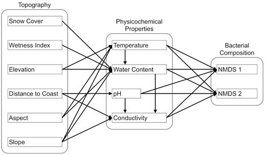
Initial a priori model of environmental factors that influence bacterial community composition in Dry Valley soils.
MATERIALS AND METHODS
Site selection, site surveys and sample collection
A study area of 220 km2, encompassing the Miers, Marshall and Garwood Valleys in the southern end of the Antarctic Dry Valleys (Fig. 2a and b), was divided using 4 primary attributes obtained by remote sensing into spatially distinct regions, termed ‘tiles’. Each tile was defined by its elevation (200 m increments from sea level to 1400 m), slope (less than or greater than 20 degrees), aspect (North-, South-, East-, or West- facing, or zero) and overriding geology (aeolian, alluvial, gneiss, granite, lacustrine, mafic, marble, moraine type 1 (M1), moraine type 2 (M2), moraine type 3 (M3), schist, scree, or complex). Tile boundaries were drawn where the combination of these environmental attributes changed. On the ground environmental assessments were completed within each tile in November 2008, to visually confirm the reliability of the remote sensing data, including the geology, and to identify microhabitats in each tile that varied from the general tile attributes. Microhabitats predominantly included stream channels, ponds and areas within tiles where the dominant tile geology varied. This process ultimately divided the landscape into 545 tiles (Fig. 2c).
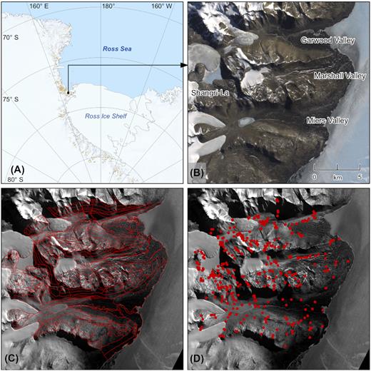
A map of the Ross Sea Region of Antarctica (A), indicating the location of the study area (B), tile boundaries (C) and sample sites (D).
During the 2008–2009 and 2009–2010 austral summers, biological surveying and soil sampling were completed at 471 sites that had been selected within tiles to capture the combination of variables that defined the tile, as well as microhabitats within the tiles that deviated from these combinations, in order to capture the environmental heterogeneity of the landscape (Fig. 2d). Soil samples for microbiological and physicochemical analyses were collected aseptically from the top 10 cm of soil below the desert pavement and stored in sterile Whirl-Packs (Nasco International, Fort Atkinson, WI, USA). At the earliest opportunity, samples for total gravimetric water content determination were transported to McMurdo Station for processing, and samples for microbiological and physicochemical analyses were frozen at −20°C to be transported to New Zealand for processing.
Determination and treatment of environmental variables
A total of six topographic variables, six physicochemical variables and two spatial variables were examined in relation to bacterial diversity and/or community composition. Topographic variables included elevation (m), aspect (degrees from North), slope (degrees), distance to the coast (m), an index of yearly snow cover and an index of soil wetness. Elevation, aspect and slope of sample sites were determined using LIDAR derived digital elevation models (Wilson and Csathó 2007). Distance to the coast was defined as the Euclidean distance of the sample site to the nearest coastline. The index of yearly snow cover and index of wetness were derived as previously described (Stichbury et al. 2011), and provide relative estimates of snow cover and liquid water availability for sites based on Geographic Information Systems (GIS) and remote sensing data. Physicochemical variables analyzed included soil pH, electrical conductivity (μS/cm), water content (w/w %), carbon content (w/w %), nitrogen content (w/w %) and average summer temperature (°C). Soil pH and electrical conductivity were determined for 2 ml of soil mixed in 10 ml of deionized water (Lee et al. 2012) using a Thermo Scientific Orion 4-Star Plus pH/Conductivity Meter (Thermo Scientific, Waltham, MA, USA). Water content was determined from the mass loss of soil following incubation at 105°C for 48 hours (Barrett et al. 2004). Organic carbon and total nitrogen content was determined from 300 mg of dried acidified soil using a CE Elantech Flash EA 1112 Elemental Analyzer (Lakewood, NJ, USA) as previously described (Barrett, Gooseff and Takacs-Vesbach 2009). Average summer temperature was predicted based on land surface temperature data from Landsat 7 ETM+ using band 6 (at 60 m resolution) and validated by field measurements (Brabyn et al. 2014). Longitude and latitude were included as spatial variables.
Data were transformed as necessary in order to address issues of skew and kurtosis. No topographic variable data was transformed prior to analysis. Soil conductivity, water content, carbon content and nitrogen content were log(x+1) transformed prior to analysis, while pH and average summer temperature were not transformed. Longitude and latitude were transformed to X and Y coordinates (m), respectively using the program ArcGIS. For the purpose of variance partitioning and spatial analyses, environmental variables were normalized using the scale function in R and environmental distance matrices based on Euclidean distances between samples were generated. Coast distance was removed as a variable in these instances to ensure that no degree of spatial variation was explicitly built into the topography and environmental distance datasets.
DNA extraction and preparation
DNA was extracted from soils as described by Barrett and colleagues (2006), with modifications to facilitate high-throughput sample processing. Briefly, 0.7 g of soil was added to a microcentrifuge tube containing 0.5 g of both 0.1 mm and 2.5 mm silica–zirconia beads (BioSpec Products, Bartlesville, OK, USA). To each sample, 270 μl phosphate buffer (100 mM NaH2PO4) and 270 μl SDS lysis buffer (100 mM NaCl, 500 mM Tris pH 8.0 and 10% SDS) were added, and samples were bead-beaten for 10 minutes on a Vortex Genie 2 with a 24-tube vortex adapter (Mo Bio Laboratories Inc., Carlsbad, CA, USA). To each sample, 180 μl CTAB extraction buffer (100 mM Tris-HCl, 1.4 M NaCl, 20 mM EDTA, 2% CTAB, 1% PVP, 0.4% BME) was added and samples were shaken at 300 rpm and 60°C for 30 minutes. Samples were centrifuged at 16 000 x g for 3 minutes, prior to the addition of 350 μl chloroform: isoamyl alcohol (24:1) and 35 μl 10 M ammonium acetate. Samples were vortexed to mix and centrifuged at 16 000 x g for 5 minutes. The aqueous phase of each sample was transferred to a 96 well lysis block and processed using an X-tractor Gene liquid handling robot (Corbett Life Sciences, Concorde, NSW, Australia), using the DX Universal liquid sample DNA Extraction Protocol (CorProtocol No. 14 104 Version 02). Samples were eluted in 80 μl TE pH 8.5 (10 mM Tris-HCl, 0.5 mM EDTA). Negative controls, consisting of bead tubes with no sample added, were processed as described above and included in each lane of the lysis block to assess potential contamination of extracts.
DNA extracts were quantified using Quant-iT Picogreen dsDNA reagent (Invitrogen, Carlsbad, CA, USA) on a FLUOstar optima fluorescence plate reader (BMG LABTECH, Ortenberg, Germany). Briefly, 100 μl of picogreen solution (picogreen diluted 1:200 in TE) was added to each well of a black 96 well plate, containing 95 μl TE and 5 μl sample or standard containing 0 to 25 ng/μl lambda dsDNA (Invitrogen). Samples were excited at 485 nm and emission was measured at 520 nm. All extracts with DNA concentrations exceeding 2 ng/μl, were adjusted to 2 ng/μl in TE.
ARISA of community DNA
PCR targeting the intergenic spacer between the 16S and 23S rRNA genes of the bacterial ribosomal operon was completed for each extraction and extraction negative controls. Each 25 μl reaction contained 1X PCR buffer, 3 mM MgCl2, 1 U Platinum Taq DNA Polymerase (Invitrogen), 0.25 μM primers ITSF (5′-GTCGTAACAAGGTAGCCGTA-3′) (Integrated DNA Technologies, Coralville, IA, USA) and ITSReub (5′-HEX-GCCAAGGCATCCACC-3′) (Applied Biosystems, Carlsbad, CA, USA) (Cardinale et al. 2004), 0.2 mM dNTPs (Invitrogen) and 5 μl of template DNA. Thermal cycling was completed on a Bio-Rad DNA Engine Peltier Thermal Cycler 200 (Bio-Rad, Hercules, CA, USA), which consisted of 3 min at 94°C; 30 cycles of 94°C for 45 s, 55°C for 1 min and 72°C for 2 min; and 72°C for 7 min (Cardinale et al. 2004). Negative extraction controls listed above and negative PCR controls were included (in which 5 μl of PCR-grade water was substitute for template DNA); these controls showed no amplification.
Amplicons were diluted 1:20 in de-ionized water. A mixture containing 2 μl of diluted amplicon, 0.13 μl of Liz-1200 internal size standard (Applied Biosystems) and 7.87 μl of HiDi formamide (Applied Biosystems) was heat denatured at 95°C for 5 minutes and cooled to 4°C for 2 minutes, before being resolved on an ABI 3130xl Genetic Analyzer (Applied Biosystems) at the University of Waikato DNA Sequencing Facility.
All peaks between 100 and 1200 base pairs in length, that made up greater than 0.3% of the entire signal over 10 rfu in each electropherogram were accepted as true peaks. The total number of true peaks was taken as a measure of bacterial taxon richness for each sample. Peaks within one base pair of one another in a pairwise comparison between fingerprints were binned together, and a Bray Curtis dissimilarity matrix using proportional peak abundance data was generated based on each pairwise comparison of the electropherograms.
Data analyses
Bivariate relationships between taxa richness and environmental variables were assessed using linear models, and significant relationships were identified using Pearson's product-moment rank correlation. Non-linear associations were identified by examining residual plots, and appropriate non-linear models were then fit based on these analyses. The amount of variation in taxa richness explained by topographic variation, physicochemical variation and spatial variation was assessed using multiple linear regression in R by applying the varpart function in the ‘vegan’ library (Oksanen et al. 2011).
Bray Curtis community dissimilarities were examined in a two-dimensional ordination using non-metric multidimensional scaling (NMDS), in order to reduce the multivariate Bray Curtis dissimilarities to compositional gradients. Ordinations were completed in R using the ‘vegan’ library (Oksanen et al. 2011). The best solution was accepted after 1000 iterations. Pearson's product-moment rank correlation between the matrix of Bray Curtis dissimilarities and a matrix of the Euclidean distances between the points in the final NMDS ordination was calculated in order to assess the amount of variation captured in the final two dimensional solution (McCune and Grace 2002). The relationships between the NMDS results and the continuous environmental variables were assessed using bivariate analyses and structural equation modeling (SEM).
Structural equation modeling (SEM) is an extension of regression and path analysis that can be used to model multivariate relations and to evaluate multivariate hypotheses (Kline 2005). Maximum likelihood solution procedures were applied using the Mplus software (v3.12) and we relied on chi-square goodness of fit measures to evaluate model adequacy. Modification indices were examined to determine if there were obvious model-data discrepancies, which in turn could be used to identify missing pathways. The model presented in Fig. 1 represents what we believed to be the most plausible structural relations based on a priori knowledge. We acknowledge that not all causal processes that act in this system are represented in Fig. 1; rather, our objective was to determine whether the data were consistent with the expectations of the proposed model. Good-fitting structural equation models do not prove causal relationships (Grace 2006). The final structural equation model predicts a covariance structure that is consistent with the covariance structure of the dataset; therefore, theory can guide our interpretation of the mechanistic nature of the directional paths. We calculated the ‘total effects’, which are the total sum of direct and indirect pathways from the predictors to composition. Indirect effects equal the total sum of the products of all path segments from a predictor to composition. Total effects provide a calculation of the net effect (i.e. strength and sign) of a relationship. Estimates of these effects and their standard errors were calculated with Mplus software (Muthén and Muthén 2005).
Spatial variation in community structure was assessed using Mantel tests and related to environmental distance using partial Mantel tests. Both tests were completed with 9999 permutations. Additionally, variance partitioning based on redundancy analysis (RDA) was used to assess the amount of variation in the community structure that was explained by topographic variation, physicochemical variation and spatial variation. In this case, the varpart function in ‘vegan’ (Oksanen et al. 2011) was used to assess the amount of variation in the Bray-Curtis dissimilarity matrix explained by matrices of topographic, physicochemical and spatial variables.
RESULTS
Patterns of bacterial richness
Bacterial richness varied significantly with several physicochemical, topographic and spatial variables (Fig. 3). Richness was most strongly positively correlated with soil water content and most strongly negatively correlated with soil conductivity. A non-linear association between bacterial taxon richness and pH revealed richness was highest around pH 8, and decreased with increasing acidity and alkalinity. Together, the physicochemical, topographic and spatial variables explained 38% of the variation in richness, with space only accounting for 1% of this variation independent of physicochemical and topographic heterogeneity (Fig. S1).
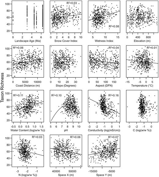
Bivariate relationships between environmental variables and bacterial taxon richness. Trend lines and r-squared values are included for significant relationships (P < 0.05).
Patterns of community structure
A two-dimensional NMDS ordination, representing similarities of bacterial community composition between sites, was reached with a stress of 0.25, and environmental gradients were assessed within the ordination (Fig. S2). Comparison of the Euclidean distances in the two–dimensional NMDS configuration and the Bray Curtis distances revealed that the final two-dimensional solution captured 66% of the variation in the community composition data. All the continuous environmental variables assessed showed significant bivariate relationships with one or both of the NMDS axes (P< 0.01) (Table 1). NMDS axis 1 was found to vary significantly with snow cover, wetness, elevation, coast distance, aspect, temperature, soil water content, pH and conductivity, but not slope. NMDS axis 2 varied significantly with snow cover, elevation, coast distance, aspect, temperature and conductivity, but not wetness, soil water content, or pH.
Bivariate correlation coefficients (r) of environmental variables with axes one and two of the non-metric multidimensional scaling (NMDS) ordination of bacterial community composition. Significant (P < 0.05) correlations are in bold.
| Variable group | Variable | NMDS Axis 1 | NMDS Axis 2 |
|---|---|---|---|
| Topography | Snow index | −0.31 | 0.16 |
| Wetness index | −0.38 | −0.04 | |
| Elevation | −0.18 | 0.35 | |
| Coast distance | −0.22 | 0.21 | |
| Slope | 0.05 | 0.24 | |
| Aspect | 0.17 | −0.14 | |
| Temperature | 0.17 | −0.20 | |
| Soil properties | Water content | −0.50 | −0.06 |
| pH | 0.29 | −0.08 | |
| Conductivity | 0.19 | −0.19 |
The initial a priori model was not consistent with the data (X2 = 242.9, d.f. = 28, P< 0.0001), and so the model was revised to find a stable final solution reflective of the relationships between the variables. Paths to soil water content from elevation, aspect and snow cover were removed, as were paths to temperature from slope, paths to pH from coast distance and paths to conductivity from pH and soil water content. Modification indices supported the addition of paths from snow cover and coast distance to temperature, paths from aspect and soil water content to pH, and paths from aspect to conductivity. Direct paths from wetness index and snow cover to community structure were also added. Finally, the variation in community structure captured in NMDS axis 2 was not explained by a unique set of variables to those explaining NMDS axis 1, so axis 2 was removed to simplify the final model.
The final model did not differ significantly from the data (X2 = 27.6, d.f. = 21, P = 0.15) and explained 43% of the variation observed in NMDS axis 1 (Fig. 4). In addition, the model explained 45% of the variation in temperature, 12% of the variation in soil water content, 11% of the variation in conductivity and 5% of the variation in pH. Soil water content had the strongest direct effect and total effect on axis 1 (Table 2). The effects of the topographic variables on community composition were largely mediated through soil property variables, with the exception of wetness index and snow cover, which had both indirect and direct effects on community composition.
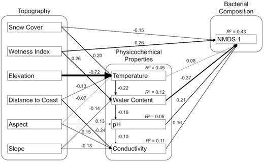
Final structural equation model (SEM) results (X2 = 27.6, d.f. = 21, P = 0.15) with standardized coefficients. All pathways were significant.
Standardized direct effects, indirect effects and total effects of environmental factors on NMDS axis one.
| Factor | Direct effects | Indirect effects | Total effects |
|---|---|---|---|
| Aspect | 0.039 | 0.039 | |
| Slope | 0.035 | 0.035 | |
| Elevation | −0.121 | −0.121 | |
| Distance to coast | −0.061 | −0.061 | |
| Snow | −0.154 | 0.034 | −0.120 |
| Wetness | −0.258 | −0.104 | −0.361 |
| Temperature | 0.080 | 0.088 | 0.168 |
| Water content | −0.370 | −0.032 | −0.402 |
| pH | 0.213 | −0.016 | 0.196 |
| Conductivity | 0.163 | 0.163 |
Spatial patterns of community structure
The average Bray Curtis community dissimilarity was found to increase with distance between samples (Mantel r = 0.103, P< 0.0001), as did environmental distance (Mantel r = 0.170, P< 0.0001) (Fig. 5). Partial correlations revealed a significant, but weak, correlation between community dissimilarity and geographic distance after accounting for environmental relationships (Mantel r = 0.058, P< 0.01). This correlation became non-significant if distance from the coast was included as a variable in generating the environmental distances (Mantel r = 0.013, P = 0.244). Variance partitioning of the community dissimilarity data also indicated that a small amount of the spatial variation in the data could not be explained by topographic and physicochemical distance (Fig. S3). The combination of physicochemical, topographic and spatial variables explained 22% of the variation in community composition.
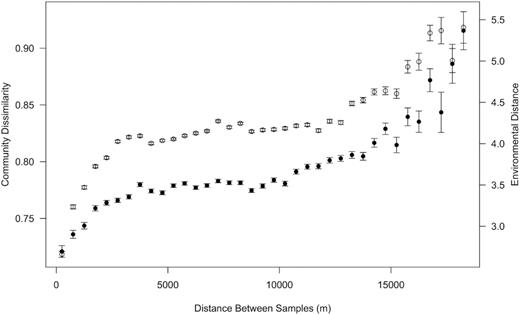
The relationship of community dissimilarity (filled circles) and environmental distance (open circles) with space. Mean variance in community dissimilarity and environmental distance were calculated between samples at 500 m intervals. Error bars show standard error. Coast distance was not included as a variable in calculating environmental distance to ensure that no degree of spatial variation was explicitly built into the environmental dataset.
DISCUSSION
Previous studies of Dry Valley soils have revealed unexpectedly diverse bacterial communities, which appear to be shaped largely by abiotic variation (Hogg et al. 2006; Cary et al. 2010; Lee et al. 2012), and which may form important linkages with higher taxa (Lee et al. 2019; Caruso et al. 2019). Here, we demonstrate that significant differences in bacterial diversity and community composition are partially explained by topographic and physicochemical properties across the Dry Valley landscape. The edaphic factors found to be most important as determinants of bacterial community diversity and composition are largely consistent with those reported from other terrestrial environments, and include soil moisture, pH and conductivity (Chu et al. 2010); however, differences in the relative influence of these variables suggest that community assembly is uniquely influenced under the environmental extremes of this cold desert landscape.
Patterns of bacterial richness
Bacterial richness was measured as the number of peaks in ARISA profiles from each sample. Despite the resolution limitations inherent to DNA fingerprinting techniques, ARISA has been accepted as a useful method for comparing taxon richness between samples (Brown and Fuhrman 2005; Fuhrman et al. 2008; Kovacs, Yacoby and Gophna 2010) and remains an important rapid, cost-effective, technique for large scale analyses of microbial communities. Diversity assessments by ARISA have been shown to agree with 16S rRNA gene diversity assessments in the McMurdo Dry Valleys (Lee et al. 2012). Applying this methodology to the current study, we detected significant variation in bacterial taxon richness with environmental gradients, and found physicochemical variables to be stronger predictors of bacterial richness than topographic variables.
Richness was most strongly negatively associated with conductivity. The importance of salinity in shaping bacterial diversity and community structure has been reported previously (Lozupone and Knight 2007), and similar negative trends in bacterial diversity with salinity have been reported in Antarctic environments (Chong et al. 2010; Zeglin et al. 2011; Magalhães et al. 2012). High salt concentrations are typical of Antarctic soils (Claridge and Campbell 1977; Vincent 2004), and in the current study conductivity values averaged approximately 0.32 mS/cm and ranged greatly from 0 to 8.3 mS/cm in soils across the landscape. Salinity presents a strong selective pressure, as few bacteria are capable of growth over large ranges of salt concentrations (Oren 2006). As such, one would expect the presence of non-halotolerant taxa to be greatly reduced in saline soils. Additionally, high soil conductivity may be indicative of sites that have been devoid of liquid water for long periods, as salts may accumulate in areas of low soil water content due to negligible leaching (Campbell and Claridge 1987). The negative association between conductivity and richness may, therefore, reflect sites of prolonged hyper-arid conditions that prohibit the establishment of many bacterial taxa.
Soil water content was the second strongest predictor of bacterial richness and wetness index was found to be the most important topographic factor explaining bacterial richness. Soil moisture and wetness index also had the strongest positive associations with bacterial richness. While soil moisture is expected to have an important influence on bacterial diversity in desert ecosystems, some recent studies have found the importance of water to be ancillary to other factors in shaping bacterial diversity in arid landscapes (Andrew et al. 2012), including the Darwin Mountains of Antarctica where soil salinity was also found to be the best predictor of bacterial diversity (Magalhães et al. 2012). As the strongest positive associations with bacterial richness, measures of soil water and areas predicted to see liquid water seasonally are likely the most important determinants of hotspots of microbial diversity in the Dry Valleys ecosystem.
Soil pH was found to be a less important predictor of bacterial richness in Dry Valley soils compared to temperate (Fierer and Jackson 2006; Griffiths et al. 2011) and Arctic ecosystems (Chu et al. 2010). These studies have described patterns of bacterial diversity in soils ranging from pH 3 to pH 9, and found richness to be highest in soils near neutral pH. Soils in the current study nearly all ranged from neutral to alkaline with greater than 95% of the values ranging from pH 7 to 10. The reduced importance of pH in shaping bacterial richness in Dry Valley soils could, therefore, be because (1) the general response in richness as pH increases from neutral is unequal to the response observed as pH decreases from neutral, (2) the smaller range of pH values observed over the landscape in the present study compared to previous reports provided an insufficient range to strongly effect richness, or (3) the harsh environmental constraints of the Dry Valley ecosystem compared to other ecosystems makes pH a secondary factor influencing richness in these soils.
Spatial trends in bacterial richness were not expected; however, significant relationships were observed with both latitude and longitude. Richness was found to increase moving North in latitude and West in longitude (with increasing distance from the coast). As expected, these spatial trends were almost entirely explained by topographic and physicochemical variation in the landscape.
Patterns of community structure
As predicted in the a priori model, the effects of most of the topographic variables on community structure were mediated through physicochemical variation. Elevation had the largest indirect effect on community composition, due to its strong effect on temperature. Variation in bacterial communities with elevation has been described previously in other systems (Bryant et al. 2008), and trends in cyanobacterial distributions have been related to elevation in the Dry Valleys (Smith et al. 2006; Wood et al. 2008). Aspect, slope and coast distance had more modest effects on physicochemical variables, with aspect found to affect temperature, pH and conductivity, while slope was found to affect water content and conductivity, and coast distance was found to affect temperature and conductivity.
Direct effects on community composition were supported for two topographic variables: snow cover and wetness index. In the a priori model, snow cover was hypothesized to impact community structure indirectly through influencing soil moisture; however, this path was not supported in the final model. It is possible that the moisture in snow rarely becomes bioavailable, as it is often removed by sublimation and strong winds rather than melting (Gooseff et al. 2003). As such, the direct impact of snow cover on community structure could be the result of the change imparted to the physical environment by shielding the soils from sunlight and ultraviolet radiation. The influence of wetness index on community composition could not be explained entirely through measures of soil moisture. As it is difficult to assess the influence of water in a soil solely by an instantaneous measure at the time of sampling, a direct path from wetness index to community composition provides a meaningful indication of potential availability of water in soils over time.
Water content and wetness index had the strongest direct and total effects on bacterial community composition. Soil moisture has been identified as the strongest predictor of bacterial community composition in recent analyses of other terrestrial systems, including soils of the Tibetan Plateau (Zhang et al. 2013), lithic communities across hot and cold hyper-arid landscapes in deserts of China (Pointing et al. 2007), and in stream sediments of the Onyx River in the Dry Valleys and Rio Salado in New Mexico (Zeglin et al. 2011). Water is understood to be a limiting variable in the Dry Valleys (Kennedy 1993; Barrett et al. 2007) and the presence of particular bacterial taxa have been related to water availability in Antarctic soils (Aislabie et al. 2006; Niederberger et al. 2008; Niederberger et al. 2015); however, the current work is the first evidence that water is the most important variable in explaining bacterial community composition in soils across the landscape as a whole.
The total effects of pH, conductivity and temperature on community composition were found to be roughly similar. Soil pH had a strong positive direct effect on community composition, but the total effects of pH were tempered slightly by a negative indirect effect mediated through conductivity. The strength of the direct and total effect of pH is not surprising, considering that pH has been found to be the most important factor shaping microbial community composition in other soils (Fierer and Jackson 2006; Lauber et al. 2009; Chu et al. 2010; Rousk et al. 2010; Griffiths et al. 2011). Conductivity, despite being the strongest predictor of bacterial diversity across the landscape, had the second smallest direct effect and smallest total effect on community composition of all the physicochemical variables analyzed. Temperature had the weakest direct effect on community composition, but a relatively strong indirect effect mediated through water content contributed to a substantial total effect. While cold-adapted bacteria may be selected for by the Dry Valley landscape as a whole, community composition within the landscape appear to show little differentiation based directly on variation in mean summer temperature. Mean summer temperatures across the landscape were predicted to range from −15 to 9°C, entirely within the psychrotrophic range (Scherer and Neuhaus 2006), providing little capacity to select different populations between sites based on different temperature optima; it is, perhaps, not surprising then that temperature has at least an equally important role in shaping community composition by influencing water availability.
Spatial patterns of community structure
A significant distance decay relationship was observed, in which community dissimilarity increased with increasing distance between samples; however, once accounting for environmental variation, the correlation, while still significant, was quite weak. Spatial variation that cannot be explained by environmental variability has been used as an indicator of dispersal limitation for bacterial populations (Martiny et al. 2011), consistent with neutral models of larger organisms (Bell 2001; Condit et al. 2002). Dry Valley landscapes are understood to be linked through aeolian and hydrological processes (Barrett et al. 2007), increasing the likelihood of dispersion of biomass over the landscape. However, recent analyses of aeolian dispersal indicate that soil bacterial communities are distinct from aerosol communities (Bottos et al. 2013; Archer et al. 2019), suggesting microbial dispersal between sites may be more limited than previously appreciated. Additionally, different prokaryotic groups may not scale uniformly across Antarctic soils, as cyanobacterial distributions exhibit spatial patterns distinct from those of the total soil bacterial community (Sokol et al. 2013). A weak trend indicating that community composition is decoupled from environmental variability may, therefore, arise from the presence of populations with varying degrees of dispersal limitation within the community. These spatial trends may be indicative of the importance of community assembly processes other than variable selection across the landscape (Stegen et al. 2012), which would be consistent with the relatively small amount of overall variation in community composition explained by environmental variables. Indeed, only 22% of the community variation was explained by the combination of physicochemical, topographic and spatial variables analyzed. Alternatively, the unexplained spatial variation reported here may be the result of environmental variation in the system that was not accounted for in this study. One must be careful not to overstate the importance of weak trends in environment-space relationships (Griffiths et al. 2011), particularly as they are known to vary with the resolution of the taxonomic data (Horner-Devine et al. 2004). A limitation of ARISA is that it does not allow identification of microbial taxa. Application of sequencing approaches that provide phylogenetic and taxonomic community information would help to resolve environmental drivers and spatial patterns of particular taxa in this system. Based on the data presented here, however, we cannot rule out the possibility that some bacterial populations show dispersal limitation across the landscape, which may have an additional effect on shaping bacterial communities to that of taxa sorting due to environmental variation.
CONCLUSIONS
At the outset of this work, three questions were asked that would help explain variation in bacterial diversity and community composition across an Antarctic Dry Valleys terrestrial landscape. Bacterial taxon richness does indeed vary with environmental gradients with soil conductivity and water content being the most important explanatory variables. Our a priori model presented paths through which environmental gradients were expected to influence bacterial community composition. Based on empirical data, this a priori model was rejected in favor of a model that supported numerous significant direct and indirect effects of abiotic variables on bacterial community composition that were not present in the initial model. Finally, a significant distance decay relationship appears to exist in soils across our study area, however, the cause of the relationship remains inconclusive, as the observed variation could not be explained entirely by environmental heterogeneity. This work provides foundational knowledge of the environmental factors influencing bacterial communities in Dry Valley soils. Such knowledge will be important locally and regionally, for shaping management strategies for Antarctica's ice free areas and predicting ecosystem responses to climate change scenarios of increased temperature, water availability and environmental variability (Wall 2007), as well as globally, in support of efforts to describe patterns in microbial ecology across the planet.
ACKNOWLEDGEMENTS
This research was supported through awards from the Foundation for Research, Science and Technology of New Zealand and the National Science Foundation (ANT 0739648) to SCC, and an award from the New Zealand Marsden Fund (UOW1003) to CKL. Logistics support for the field seasons was provided by Antarctica New Zealand. We especially thank the many researchers who were involved in the New Zealand Terrestrial Antarctic Biocomplexity Survey (nzTABS) for their time and commitment to this work.
Conflict of interest. We declare no conflict of interest.
REFERENCES
Author notes
Department of Biological Sciences, Thompson Rivers University, Kamloops, BC, Canada.
Division of Microbial Ecology, Centre for Microbiology and Environmental Systems Science, University of Vienna, Vienna, Austria.
Department of Botany, University of Wyoming, USA.
