


Abstract
Despite decreasing costs, generating large-scale, well-replicated and multivariate microbial ecology investigations with sequencing remains an expensive and time-consuming option. As a result, many microbial ecology investigations continue to suffer from a lack of appropriate replication. We evaluated two fingerprinting approaches – terminal restriction fragment length polymorphism (T-RFLP) and automated ribosomal intergenic spacer analysis (ARISA) against 454 pyrosequencing, by applying them to 225 polar soil samples from East Antarctica and the high Arctic. By incorporating local and global spatial scales into the dataset, our aim was to determine whether various approaches differed in their ability and hence utility, to identify ecological patterns. Through the reduction in the 454 sequencing data to the most dominant OTUs, we revealed that a surprisingly small proportion of abundant OTUs (< 0.25%) was driving the biological patterns observed. Overall, ARISA and T-RFLP had a similar capacity as sequencing to separate samples according to distance at a local scale, and to correlate environmental variables with microbial community structure. Pyrosequencing had a greater resolution at the global scale but all methods were capable of significantly differentiating the polar sites. We conclude fingerprinting remains a legitimate approach to generating large datasets as well as a cost-effective rapid method to identify samples for elucidating taxonomic information or diversity estimates with sequencing methods.
Introduction
The microbial ecology landscape has been revolutionised by culture-independent methods. In particular, sequencing technologies have been responsible for exposing the previously unknown rare biosphere (Sogin et al., ). Since the landmark Global Ocean Sampling expedition began in 2003 (Rusch et al., ), key developments including high-throughput capabilities, multiplexing technologies and miniaturisation of sequencing chemistries continue to reduce the time and costs involved with sequencing (MacLean et al., ). The greater affordability and accessibility of next-generation sequencing (NGS) technologies such as massively parallel pyrosequencing has seen the volume and the application of sequencing dramatically increase from marine, terrestrial and extreme environments, to medical and artificial systems such as wastewater treatment plants (Nowrousian, ; Zhou et al., ; Novais & Thorstenson, ; Zhang, ). Examination of natural and engineered microbial ecosystems using NGS is now prolific throughout the literature, with the trend likely to continue.
With increased application of pyrosequencing and other high-throughput sequencing technologies, inaccuracies due to PCR biases (Gihring et al., ; Pinto & Raskin, ), sequencing errors (Quince et al., ) and high numbers of chimeras (Kunin et al., ) have also become increasingly apparent (Pinto & Raskin, ). Improvements in processing software (Huse et al., ; Edgar et al., ; Davenport & Tummler, ) and technological advances continue to address many of these limitations. However, some of the most significant shortfalls highlighted in microbial ecology studies are not associated with technology per se, but originate from poor experimental design, often the result of resource limitations (Prosser, ). Consequently, there is now greater scrutiny and criticism of experimental design and comparative community diversity analyses, with lack of replication and poor experimental design attracting particular attention (Bent & Forney, ; Prosser, ). Despite being more affordable than ever, delivering a large-scale, well-replicated, multivariate microbial diversity investigation with NGS remains an expensive and time-consuming option, requiring significant bioinformatic processing power and skill.
Genotypic fingerprinting techniques are an established set of molecular tools used to rapidly profile microbial communities in a variety of systems (Singh et al., ; Bissett et al., ; Sun et al., ). They include single-strand conformation polymorphism (SSCP), automated ribosomal intergenic spacer analysis (ARISA), temperature gradient gel electrophoresis (TGGE), denaturing gradient gel electrophoresis (DGGE) and terminal restriction fragment length polymorphism (T-RFLP). Unlike sequencing technologies, genotypic fingerprinting does not provide direct taxonomic information, though in the case of DGGE and less frequently T-RFLP (Pilloni et al., ) and ARISA (Brown et al., ), the data output can be analysed further to obtain sequence identification. Limited capacity to capture the presence of rare taxa and the inaccuracy of genotypic fingerprinting-based abundance estimates are well-described limitations of fingerprinting techniques (Bent et al., ). Furthermore, variations between analyses and semiquantitative results have been suggested to hinder robust comparisons between studies and even investigators (Dunbar et al., ; Osborne et al., ).
Despite these limitations, the use of fingerprinting methods to provide rapid and relatively inexpensive community profiles remains widespread (Bissett et al., ; Giebler et al., ; Neumann et al., ). A number of small scale investigations have recently demonstrated consistent microbial community structures generated from fingerprinting and pyrosequencing methods. Gillevet et al. () used 454 pyrosequencing based analysis of the 16S rRNA gene (or ‘16S tag sequencing’) to confirm that ARISA fungal profiles may represent multiple taxa and a given taxon may be represented by more than one operational taxonomic unit (OTU). Despite this, fungal community trends associated with four salt-marsh plants across six time points (n = 24) were still consistent between ARISA and 16S tag pyrosequencing methods (Gillevet et al., ). Similarly, Pilloni et al. () observed that T-RFLP and 16S tag sequencing recovered similar microbial community structures from a contaminated aquifer and highly reproducible read abundances across biological and technical replicates (n = 9; Pilloni et al., ). While Cleary et al. () reported consistent patterns across composite samples of four rhizosphere environments (nursery, nursery transplant, native and mangrove) using DGGE data and 16S tag sequencing data (Cleary et al., ).
The aim of this study was to investigate the sensitivity of one commonly used NGS platform – 454 Titanium tag pyrosequencing against two genotypic fingerprinting techniques, T-RFLP and ARISA. We chose to use a large sample set of 225 polar soils obtained from across East Antarctica and the high Arctic, to incorporate local (centimetres to hundreds of metres) and global (kilometres to thousands of kilometres) spatial scales. We compared the ability of these culture-independent techniques to detect similarities in biological assemblages and to correlate these similarities with variations in environmental variables. T-RFLP was selected because it targets the same genetic marker (16S rRNA gene) as our NGS approach, allowing direct comparison between the two. ARISA, which targets the ITS region, was selected based on its reportedly greater taxonomic resolution than T-RFLP (Danovaro et al., ). We hypothesised that the NGS approach would provide far greater resolution than either of the fingerprinting methods, but that all methods would provide similar community structure patterns.
Methods
Site descriptions and sampling design
In total, eight polar locations were selected (Fig. 1). Five sites from Antarctica (Fig. 1b); Mitchell Peninsula denoted Mitchell (66°31′S, 110°59′E), Casey Station denoted Casey (66°16′S, 110°31′E), Robinson's Ridge, denoted RT (66°22′S, 110°35′E), Herring Island denoted Herring (66°24′S, 110°39′E) and Browning Peninsula denoted Browning (66°27′S, 110°32′E). Three sites from the high Arctic (Fig. 1a); Alexandra Fjord Highlands, Canada denoted C_AFH (78°51′N, 75°54′W) Spitsbergen Longyearbyen Slijeringa, Norway denoted N_SS (78°14′N, 15°30′W) and Spitsbergen Longyearbyen Vestpynten, Norway denoted N_SV (78°14′N, 15°20W). At each site, a variable-lag distance geospatial design was used to collect 93 samples. Three parallel transects 300 m long and 2 m apart were established as outlined in Banerjee and Siciliano () (Fig. 1c). Soil samples were collected at 31 points (0, 0.1, 0.2, 0.5, 1, 2, 5, 10, 20, 50, 100, 100.1, 100.2, 100.5, 101, 102, 105, 110, 120, 150, 200, 200.1, 200.2, 200.5, 201, 202, 205, 210, 220, 250 300 m) along each transect. This design allows fine-scale (0–1 m), medium-scale (1–10 m) and large-scale (10–300 m) spatial patterns of microbial communities to be captured. For this investigation, all samples from the Mitchell Peninsula were characterised (n = 93) and a subselection of samples was included from the other seven sites (n = 18/24 per site), resulting in a total of 225 samples.
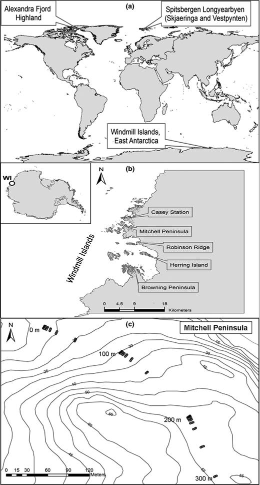
Map of sampling site locations. (a) Global map of the polar sampling sites from the high arctic and East Antarctica. (b) Location of the five East Antarctic sampling sites. (c) Transect and sample locations at Mitchell Peninsula.
Physical and chemical data collection
Physical and chemical data were collected concomitantly for each soil sample. Briefly, pH and conductivity were measured using a 1 in 5 soil to distilled water suspension. Grain size of the soils was measured by removing particles larger than 2 mm (gravel) then separating particles based on size into silt (< 63 μm) and sand (63–2000 μm). The particle size ranges were measured using laser scatter and the percentage of the total soil for each fraction calculated. Total Kjeldahl digested phosphorus and nitrogen were measured as well as total carbon by combustion and NDIR gas analysis (Rayment & Lyons, ). The water extractable chemicals (  , Br−,
  ,
,  ,
,  , and
, and  ) were obtained with a 1 in 5 dilution of soil to distilled water on a dry-matter basis [mg kg−1]. Anions were analysed by ion chromatography, and ammonium cation concentration was measured by the colorimetric indophenol method. Measurement of major elemental concentrations (SiO2, TiO2, Al2O3, Fe2O3, MnO, MgO, CaO, Na2O, K2O, P2O5, SO3 and Cl) was performed using X-ray fluorescence (XRF) analysis. Additional site parameters including slope gradient, slope aspect and elevation were derived from the GPS information using gis software and a site digital elevation model.
DNA extraction
Approximately 0.25–0.30 g of soil was used for DNA extraction using the FastDNA SPIN kit for soil (MP Biomedicals, NSW, Australia) as per the manufacturer's instructions. Each of the 225 polar soils was extracted in triplicate. DNA was quantified with Picogreen (Life Technologies, Vic., Australia) and fluorescence measured on a fluorescence plate reader (SpectraMax M3 Multi-Mode Microplate Reader; Molecular Devices, CA).
Bacterial ARISA
The three replicate DNA extracts for each of the 225 samples (n = 675) were titrated to a standard working concentration (10 ng μL−1). The DNA was amplified by PCR targeting the ITS region with the universal primers 1392f; 5′ GYACACACCGCCCGT3′ and a 5′MAX labelled 23Sr 5′GGGTTBCCCCATTCRG3′ (Fisher & Triplett, ; Hewson & Fuhrman, ). The 25 μL reaction contained 0.5 μM of each primer, 1 unit of Taq polymerase (Promega), 1× buffer (Promega), 2.5 mM MgCl2 (Promega), 0.25 mM of each dNTP (Promega) and 0.8 μg μL−1 of BSA. The reaction was held at 94 °C for 2 min followed by 30 cycles of amplification at 94 °C for 30 s, 55 °C for 30 s and 72 °C for 30 s, with a final extension at 72 °C for 5 min (Slabbert et al., ). Fragment length separation was performed at Macquarie University on an Applied Biosystems 3730 fragment analyser (Life Technologies) and subsequently interpreted via genemapper software (Life Technologies). The fragments were further filtered to separate and remove background fluorescence from true peaks in the t-rex (T-RFLP analysis Expedited) online software using the default parameters (Culman et al., ). The filtered data were used as input to a custom fragment length binning script (Ramette, ) in r v2.10.1 (R Development Core Team ). Fragments were assigned to bins of 2 base pairs [±1 base pairs (bp)] for fragments up to 700 base pairs length, bins of 3 base pairs for fragments between 700 and 1000 base pairs length and bins of 5 base pairs for fragments above 1000 base pairs (Brown et al., ). The final data output was transformed into a peak area verses sample matrix, with each peak assumed to represent an OTU (Brown et al., ; Hewson & Fuhrman, ).
The intrasample similarity between replicates was evaluated through a Bray–Curtis similarity matrix, nMDS ordinations and a cumulative rank abundance curve in primer 6 and by comparing the shared and unique OTUs between replicates. After confirming a strong correlation between the technical replicates, one DNA extract from each of the 225 soils was selected at random as a representative for further ARISA analysis and for both 454 sequencing and T-RFLP.
Roche 454 FLX Titanium pyrosequencing
The selected gDNA from each of the 225 soils was sent to an external facility (Research and Testing Lab, Lubbock, TX) for amplicon sequencing on the 454 FLX titanium platform (Roche, Branford, CT). The DNA was used as a template for amplification of the 16S rDNA gene with the universal primers, 28F and 519R (Dowd et al., ). Raw data were provided in the form of standard flowgram format (sff) files. The sequences and flowgrams were extracted from the sff files, demultiplexed and error-checked via the Pyronoise algorithm (Quince et al., ) in mothur (Schloss et al., ). Further quality screening of the sequence data included removing short reads (< 150 bp), homopolymers (> 8 bp repeats) and truncation of 16S reads > 450 bp, followed by dereplication for ease of computation. Chimera checking with the UCHIME algorithm (Edgar et al., ) allowed removal of any other erroneous sequences, and sequences were preclustered at 1% to account for 454's titanium instrument error rate (Huse et al., ).
Bacterial seed sequences were aligned to the curated SILVA secondary structure alignment (Pruesse et al., ). Aligned 16S sequences were then clustered into OTUs based on 96% sequence similarity as the best definition for species-level OTUs in this region of the 16S rDNA gene (Lane, ). An OTU abundance-by-sample matrix was generated from the bacterial dataset with mothur (Schloss et al., ). As an additional stage of quality control, global 16S rDNA gene sequence singletons were removed from the dataset.
T-RFLP
The identical gDNA template used for 454 was also used for T-RFLP analysis. Again, the 28F and 519R primers were used to amplify the 16S rDNA gene as described (Singh et al., ). Each 50 μL PCR contained gDNA template, 1 mM MgCl2, HPLC-purified primers, buffer, 1 U of Taq DNA polymerase (Qiagen), 50 mM of each dNTP (Promega). The PCR comprised 1 cycle of 94 °C for 3 min; 30 cycles of 94 °C for 30 s, 55 °C for 30 s and 72 °C for 60 s, and a final extension step of 72 °C for 10 min. PCR amplicons were isopropanol precipitated, quantified as above and 70 ng digested with the restriction endonucleases HinFI. Digests were isopropanol precipitated, resuspended in 10 mL formamide containing LIZ600 size standard (Applied Biosystems), denatured at 95 °C (3 min) and separated by capillary electrophoresis (ABI PRISM3130xl Genetic 110 Analyser; Applied Biosystems). The fragment outputs were interpreted with genemapper software (Life Technologies) and further analysed with TREX and the interactive binner script as above. Any peaks greater than the fragment size (500 bp) were removed, resulting in a peak verses sample matrix, with each peak assumed to represent an OTU.
Correlation between methods
The biological datasets generated from the three methods were imported into primer 6 for multivariate analysis (Clarke & Warwick, ). The OTU abundance-by-sample matrices were transformed (square root) and a series of alpha diversity indices calculated. Margalef's index (d), OTU richness (S), Pielou's evenness (J’), Shannon index (H’) and the Simpson index (λ) were used to evaluate the variability of diversity indices between datasets. Rarefaction curves were calculated for each site. The OTU abundance-by-sample matrices were then standardised to give relative OTU abundances (%). A dissimilarity matrix for each dataset was calculated using the Bray–Curtis coefficient, and principal component ordination (PCO) plots were created to visualise the ordering of the samples in reduced (2D) space. The co-ordinates of the first principal component (PCO1) were compared to evaluate the correlation between PCO plots. To further test the correlation of the similarity matrices, Mantel correlations were calculated with the RELATE function in primer. The potential to distinguish between a priori groups was evaluated with analysis of similarity (anosim; Clarke, ), using 999 permutations and assuming α = 0.05.
Correlation with environmental variables
The physical and chemical data were transformed based on the distribution of the data. Variables that were right-skewed (elevation, slope, conductivity,  ,
,  , SiO2, Al2O3, MnO, CaO, P2O5, SO3, Cl, moisture,
  , N and P) were log-transformed, while the water extractable
  and Fe2O3 were transformed by the square root. The resulting environmental data matrix was normalised (mean/SD) to reduce the data to a consistent scale. The correlation of the environmental parameters with the biological distributions in each PCO plot was calculated with Pearson's coefficient and displayed in a radar plot. The values from some environmental parameters that were logically related and generated similar results were combined as an average, as indicated on the plot (CaO & MgO, TiO2 & SiO2, Na2O & K2O, Al2O3 & Fe2O3). Further, a distance-based redundancy analysis (Legendre & Anderson, ) using the Primer routine DistLM was utilised to determine the predicator capacity of each variable analysed individually (marginal) and in combination with other variables (sequential). The selection criterion used was the adjusted R2, and the model selection procedure was stepwise. A stepwise procedure allows each variable to be added and eliminated with a conditional test performed at each stage to identify any improvements in the selection criteria. The stepwise selection procedure only stops once no further improvements in the selection criteria can be made. The values were added in order of the above correlation.
Modification of matrices
To evaluate the effect of OTU abundances, all of the data were transformed to binary presence/absence matrices and the analyses were repeated. To investigate the proportion of the community driving the major biological patterns, four new reduced matrices were created with OTUs contributing > 1%, > 10%, > 15% and > 20% of the total abundance. To further investigate similarities and dissimilarities between the T-RFLP data and the pyrosequencing data, an in silico evaluation was generated in TRiFle (Junier et al., ) based on the pyrosequencing sequences. The resulting predicted data were compared with the experimental data and presented as modified data matrices.
Results
Intrasample variation
There were strong biological similarities between replicate ARISA samples observed in the NMDS ordinations (Fig. 2a). Comparisons of shared and unique OTUs between replicate ARISA samples further confirmed a significant correlation with 98% of the total abundance consistent between all replicates. Those OTUs found in two or fewer replicates contributed < 2% of total abundance (Fig. 2b). A strong correlation of the replicates across the whole dataset was also observed in the cumulative rank abundance curves (Fig. 2c).
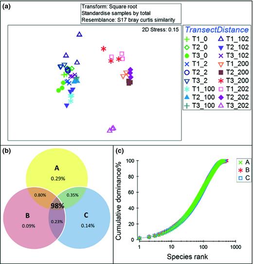
Correlation between technical replicates generated with ARISA. (a) The biological similarity between replicate samples for Alexandra Fjord Highland. (b) Relative abundance of shared and unique OTUS between the replicates across the entire dataset. (c) The cumulative rank abundance curves for replicates A, B and C across the entire dataset.
OTU abundances
The pyrosequencing approach retrieved greater numbers of OTUs than either of the fingerprinting methods by approximately an order of magnitude (Table 1). The average number of reads for all the sites processed with the 454 pyrosequencing was 3705.0 (491.5 SE), with an average OTU richness (S) of 585.0 (51.5 SE). The average number of OTUs/fragments obtained per site with genotypic fingerprinting was 99.8 (0.1 SE) for ARISA and 95 (0.5 SE) for T-RFLP, with an average OTU richness of 48.0 (3.0 SE) and 65.0 (1.6 SE), respectively. Overall, the genotypic fingerprinting captured 8–11% of the OTU richness obtained with pyrosequencing. The rarefaction curves did not reach an asymptote for any of the sites indicating the current sequencing effort was not sufficient to capture the total diversity present (Fig. 3). The Antarctic sites (Casey, Browning, RT, Mitchell and Herring) were closer to reaching the asymptote of the rarefaction curves than the high Arctic sites (C_AFH, N_SS and N_SV) suggesting lower biodiversity. This lower diversity present at the Antarctic sites compared with the Arctic sites was only reflected in the 454 pyrosequencing generated diversity, richness and evenness estimates.
Calculated diversity estimates for each polar site
Margalef's Diversity index.
Pielou's Evenness index.
Shannon Diversity index.
Calculated diversity estimates for each polar site
Margalef's Diversity index.
Pielou's Evenness index.
Shannon Diversity index.
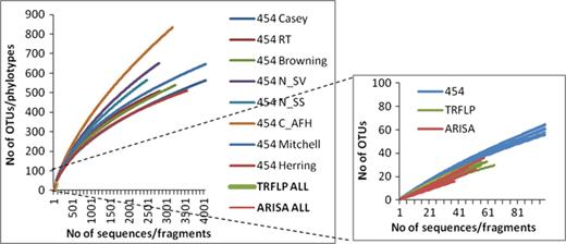
Rarefaction curves calculated for each site based on the 454 pyrosequencing, T-RFLP and ARISA results.
Correlation between pyrosequencing and fingerprinting methods
The OTU richness for each of the 225 samples was compared between methods. The richness showed no correlation between the 454 pyrosequencing and either of the fingerprinting methods, nor did the OTU richness correlate between the two fingerprinting approaches (Table 1; Supporting Information, Fig. S1). Similarly, the fingerprinting methods did not generate the same diversity trends as the 454 pyrosequencing, or each other (Table 1).
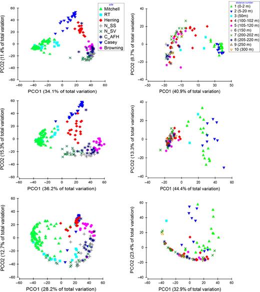
There was a strong resemblance between the principal component plots (Fig. 4) and a strong correlation of the PCO1 coordinates between all methods (R2 = 0.88, 0.63, 0.60; Fig. S1). The complexity and volume of the datasets made visualisation in low dimensionality (2D) difficult, with only 22–29% of the total variation within the resemblance matrix explained by PCO1 and PCO2 for the complete dataset, and 29.7–40% for the Mitchell Peninsula subset (Fig. 4).
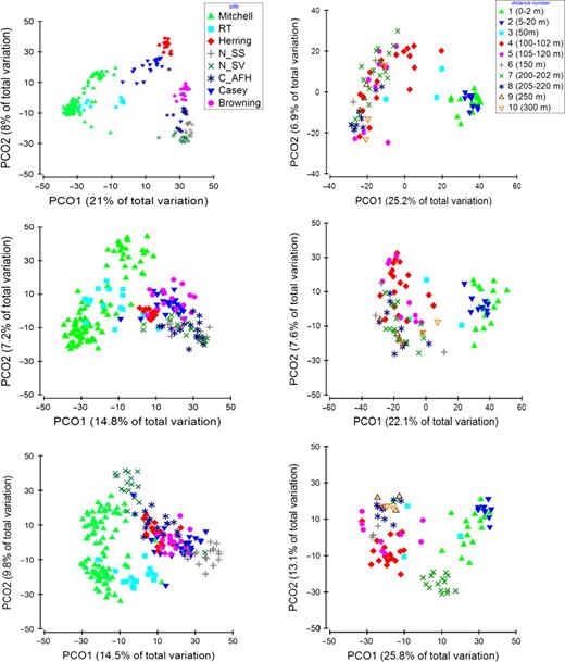
Comparison of the PCO plots generated with the 454 pyrosequencing, ARISA and T-RFLP results. The first 3 PCO plots represent all samples, separated by sites. The following three plots represent all the samples within the Mitchell Peninsula site, separated by the a priori distance groups.
Comparisons of the similarity matrices with MANTEL tests confirmed significant resemblances between the datasets (Table 2). The matrices from the 454 pyrosequencing and ARISA platforms were most similar (ρ= 0.62, P <0.001). The similarity matrices from Mitchell Peninsula were also correlated, with the 454 and ARISA technologies again generating the most similar matrices (ρ = 0.72, P <0.001). Simplifying the data to presence/absence increased the correlation between the 454 and the T-RFLP datasets from ρ= 0.46 to ρ= 0.62 (P < 0.001). Only small variations were seen for other binary matrices.
MANTEL tests results (testing the similarities of the matrices)
Presence/absence.
MANTEL tests results (testing the similarities of the matrices)
Presence/absence.
Differentiating a priori groups
All methods were capable of separating (α = 0.05) samples based on site (Fig. 4, Table 3). The 454 data had the greatest resolution at the global scale, generating the highest R value of 0.90 (P <0.001), with 8/20 of the pairwise results generated the maximum R statistic of 1 for individual site comparisons (Table 3). The global R values for the ARISA and T-RFLP were 0.67 and 0.760 (P < 0.001). The reduction in the data to presence/absence did little to vary the results (Table 3). All methods were capable of detecting differences between distance groups (based on sampling distances within sites), with global R values of 0.64 to 0.57 (P <0.001; Table 3). However, the distance groups 4–10 (Table 4) could not be significantly separated in individual pairwise comparisons. The reduction in the data to presence/absence slightly improved the global value for the 454 pyrosequencing data (R = 0.61, P < 0.001) and the T-RFLP data (R = 0.68, P < 0.001), yet the distance groups 4–10 were still not significantly resolved (Table 3).
anosim between methods (testing the ability to distinguish between a priori groups)
Distance groups (2 = 5–20 m, 4 = 100–102 m, 5 = 105–120 m, 6 = 150 m, 7 = 200–202 m, 9 = 250 m; see Table 4).
anosim between methods (testing the ability to distinguish between a priori groups)
Distance groups (2 = 5–20 m, 4 = 100–102 m, 5 = 105–120 m, 6 = 150 m, 7 = 200–202 m, 9 = 250 m; see Table 4).
Distance groups delineated a priori based on sampling distances within sites
| Group number | Distance range (m) | Sampling distances included (×3 Transects) (m) |
| 1 | 0–2 | 0, 0.1, 0.2, 0.5, 1, 2 |
| 2 | 5–20 | 5, 10, 20 |
| 3 | 50 | 50 |
| 4 | 100–102 | 100, 100.1, 100.2, 100.5, 101, 102 |
| 5 | 105–120 | 105, 110, 120 |
| 6 | 150 | 150 |
| 7 | 200–202 | 200, 200.1, 200.2, 200.5, 201, 202 |
| 8 | 205–220 | 205, 210, 220 |
| 9 | 250 | 250 |
| 10 | 300 | 300 |
Environmental predictor variables
With similar resemblance patterns between the biological datasets, similar correlations to the environmental data were expected. The T-RFLP data were found to have the weakest correlation with the environmental data, particularly with conductivity and SO4 (Fig. 6). In contrast, the correlations with phosphorus,  and P2O5 were greater in the T-RFLP data than in the other two datasets (Fig. 6). The most significant environmental variables generated within the sequential DistLM [Grain size (min), pH, Latitude, TiO2, MnO, Elevation, PO4, Cl, Carbon, Aspect, Slope and Longitude] were consistent across the methods, although there were some slight variations in the ranking of variables (Table 5). The total variance explained by all 47 measured variables was 62.6% (454), 51% (ARISA) and 59% (T-RFLP). Environmental correlations with the PCO1 axis co-ordinates were calculated individually, while the sequential tests in DistLM generated a parsimonious subset of variables that best explained proportions of the variation. DistLM placed less emphasis on longitude, moisture, mud,
  , Na2O, K2O and other grain size measurements suggesting a level of co-variance with other variables and more emphasis on elevation,
  , aspect, slope and carbon.
The major environmental variables contributing to biological variation from distance-based redundancy models (as calculated in sequential DistLM)

All environmental variables listed were significant (α = 0.05). Variables explaining more than 1% of the proportional biological variation are listed in bold.
Total cumulative variation explained for the best DistLM model generated.
The major environmental variables contributing to biological variation from distance-based redundancy models (as calculated in sequential DistLM)
All environmental variables listed were significant (α = 0.05). Variables explaining more than 1% of the proportional biological variation are listed in bold.
Total cumulative variation explained for the best DistLM model generated.
Modified data matrices
The reduction in the data to a binary form did little to alter the MANTEL and anosim results (Tables 23, S1, S2). Subsampling the pyrosequencing dataset to OTUs contributing > 1%, > 10%, > 15% and > 20% of the abundance showed that the major biological patterns were defined by very few, highly abundant OTUs (< 0.25%; Fig. 5 and Tables S1 and S2). Retaining only those OTUs contributing more than 15% of the total abundance (17 OTUs) led to a deterioration of the patterns and the ordinations bore little resemblance to the original data (Fig. 5 and Tables S1 and S2). However, the Mantel tests and anosims still produced similar patterns to the full datasets. With only those OTUs responsible for more than 20% of the total abundance (10 OTUs), the patterns had completely broken down and differentiation between a priori groups was no longer possible (Tables S1 and S2).
Comparison of the PCO plots generated from the reduced 454 pyrosequencing matrices of OTUs contributing > 1%, > 10% and > 15% of the total abundance. The first three PCO plots represent all samples, separated by sites. The following three plots represent all the samples within the Mitchell Peninsula site, separated by a priori distance groups.
In Silico verses experimental T-RFLP
The in silico T-RFLP results varied from the actual experimental T-RFLP results, yet the two were still significantly correlated (ρ = 0.46, P < 0.001). As expected, the in silico T-RFLP results resembled the 454 data (ρ = 0.79, P < 0.001) and had a similar capacity to distinguish between groups as the modified 454 matrix reduced to OTUs contributing > 10%. The numbers of OTUs from the 454 pyrosequencing data represented by each fragment size ranged from 1 to 1512, with an average of 100 OTUs per fragment. A total of 182 individual fragment sizes were generated, ranging from 20 to 308 bp. In comparison, the final experimental T-RFLP and ARISA generated 350 and 661 fragment sizes ranging from 150 to 500 bp and 350 to 1500 bp, respectively.
Discussion
Currently, 454 pyrosequencing is the most widely used NGS method for characterising microbial communities (Claesson et al., ; Zinger et al., ). We found that ARISA and T-RFLP displayed comparable sensitivity to 454 pyrosequencing, exhibiting the ability to differentiate between polar sites at a global scale and the local scale of metres to hundreds of metres. The fingerprinting methods were also highly reproducible as seen by the strong biological correlation observed between the technical replicates (Fig. 2). In comparison with the NGS approach, fingerprinting was a cheap and rapid alternative, ideal for ensuring appropriate replication in large microbial ecology studies (Table 6).
Summary of microbial community analysis methodologies (Information is based on results from this investigation, correct at the time of publishing)
| 454 sequencing | T-RFLP | ARISA | |
| Target phylogenetic gene | 16s rRNA | 16s rRNA | ITS |
| Average cost (per sample) | AU $100 | AU $10 | AU $10 |
| Potential for bias | PCR bias Chimeras Sequencing errors | PCR bias Inaccurate binning Excludes species in low abundance | PCR bias Inaccurate binning Excludes species in low abundance |
| Reliable diversity estimates | Yes | No | No |
| Reliable community structure analysis | Yes | Yes | Yes |
| Reliable links with environmental variables | Yes | Yes | Yes |
The fingerprinting methods generated ∼10% of the OTU numbers recovered with pyrosequencing. We demonstrated here that the saturation point of the analysis at 100+ fragments per sample limited the ‘dynamic range’ (Bent & Forney, ), which restricted the upper ranges of the richness gradient. This prevented correlation between the fingerprinting and pyrosequencing generated richness estimates (Fig. S1). While previous investigations have reported higher richness and diversity estimates with ARISA over T-RFLP (Danovaro et al., ), we found here that the two fingerprinting methods generated variable yet statistically equivalent diversity estimates with no correlation to the pyrosequencing results, or to each other (Hartmann & Widmer, ). In line with previous investigators (Bent et al., ; Gillevet et al., ), we have confirmed that diversity estimates from fingerprinting methods likely severely underestimate alpha diversity and thus are inappropriate for comparisons across microbial ecology investigations.
Despite less resolution at the global scale, the fingerprinting methods had a similar capacity to capture significant biological patterns and correlate environmental variables with biological distributions as the pyrosequencing data. By progressively reducing the pyrosequencing data to the most abundant sequences, we found that the observed biological patterns were driven by a very small proportion of the most abundant OTUs, with the major biological patterns disintegrating only after all but 10 to 17 of the original 17 000 OTUs remained (∼0.1%). This was further supported by the binary transformation (up weighting the importance of rare OTUs), which had no real effect on the observed biological patterns, re-enforcing the practical potential of molecular fingerprinting methods to capture major biological patterns. It is important to note that we did not saturate the rarefaction coverage curves and that if we did rarer OTU's may contribute more to general patterns. Yet, even very large sequencing efforts often fail in this regard (Gilbert et al., ) and will likely continue to fail to fully sample most communities. Additionally, it is important to note that distance-based analyses such as Bray–Curtis are dominated by the most variable species or OTUs. It has been reported that as mean abundances increase, variance also tends to increase. Therefore, the resulting resemblances even in the full dataset may be disproportionally driven by abundant organisms, despite the transformations, as a result of an underlying mean–variance relationship (Warton et al., ).
The most significantly correlated environmental parameters linked to the bacterial composition at the eight polar sites investigated here were minimum grain size, pH, longitude and latitude, and to a lesser extent the elevation, aspect, MnO,  , carbon, moisture and
  (Table 5, Fig. 6). While these results were observed for all three methods, the T-RFLP data were variable in its community correlation to environmental data, and we were unable to identify individual sites or samples responsible for this variation. The pH has been widely linked to bacterial community composition (Fierer & Jackson, ; Lauber et al., ) along with other nutrient or soil fertility factors such as organic matter, nitrogen and chloride content (Grayston et al., ; Allison et al., ). As we focused primarily on the global scale for the environmental correlations, it was unsurprising that only global spatial measurements were significant. The role of spatial distance and abiotic factors on microbial community composition has been reported to be dependent on scale (Bissett et al., ; Martiny et al., ; Van Horn et al., ), and we acknowledge that the relative influence of the environmental factors may differ at local and regional scales.
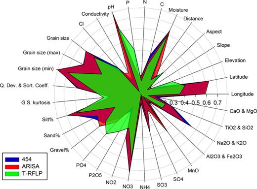
Correlation of the environmental parameters with the biological datasets for 454 pyrosequencing, ARISA and T-RFLP datasets. Correlation values were calculated against the PCO1 axis with Pearson's correlation.
Despite targeting the ITS gene (instead of the 16S rRNA gene), the ARISA results were more consistent with those produced from the 454 pyrosequencing data than the T-RFLP. This is likely due to the fact the ITS region is a noncoding region with greater variability in the nucleotide sequence than the 16S rRNA gene (Guasp et al., ; Danovaro et al., ). Previous studies have found ARISA is capable of discriminating at the species level (Hewson & Fuhrman, ), while T-RFLP is capable of discriminating at the genus level only (Guasp et al., ). ARISA has also been found to have a greater capacity than T-RFLP to detect genera that contribute < 5% of the abundance in aquatic environments (Danovaro et al., ). Without further analysis, it is difficult to confirm the resolution of ARISA and how many taxa may be represented by each operational taxonomic unit as in Gillevet et al. (). However, the in silico T-RFLP results confirmed a relative lack of resolution, with an average of 100 pyrosequencing generated OTUs collectively binned in every in silico T-RFLP generated OTU.
With no taxonomic identification and community structure information constrained to the most abundant organisms, fingerprinting can be a restricted molecular tool. For example, in Musat et al. (), organisms present in low abundance (∼0.3%) were shown to contribute more than 40% of the total uptake of ammonium and 70% of the total uptake of carbon from the environment a finding that would have been missed or masked by patterns from the dominant few. However, it is important to recognise, particularly in microbial ecology, that taxonomic identification is not always more informative. If the taxonomic identities are pursued, as they often are, at the cost of replication, then there is a reduced or nonexistent capacity to detect significant environmental patterns. Fingerprinting methods can be used to ensure statistical robustness in comparing patterns (identifying the spatial scale or environmental drivers), as well as to inform further targeted analysis using more expensive, higher resolution methods. For example, Winter et al. () used T-RFLP profiles to confirm that bacterial and archaeal community composition in subpolar and Arctic waters was significantly correlated with environmental conditions, yet not by spatial distance (Winter et al., ). While in Bissett et al. (), fingerprinting with T-RFLP was used to establish spatial, environmental and geographic patterns before combining samples to target for PhyloChip analysis.
It is our suggestion that fingerprinting should not be left out of the molecular tool kit in place of NGS approaches if sequencing cannot be conducted at a level of replication that guarantees appropriate power and inference. With fingerprinting methods capable of detecting significant spatial (as seen here), temporal (Gillevet et al., ) and treatment (Cleary et al., ) shifts in communities similarly to pyrosequencing data, full-scale sequencing is not necessary to monitor community structural changes (Prosser, ). We conclude that genotypic fingerprinting provides an independent and legitimate molecular tool for the generation of large, statistically robust biological patterns (Winter et al., ). Additionally it offers a rapid, relatively inexpensive option to judiciously select appropriate samples for further phylogenetic analysis, based on statistically significant pattern information.
Acknowledgements
The authors would like to thank the Australian Antarctic Division for financial and logistical support towards the successful collection of the polar soils. This research was supported by Australian Antarctic Science Grant AAS 2952.
References
Author notes
Editor: Johanna Laybourn-Parry
Australian Antarctic Science
AAS 2952
