


Abstract
Organisms that are adapting to long-term environmental change almost always deal with multiple environments and trade-offs that affect their optimal phenotypic strategy. Here, we combine the idea of repeated variation or heterogeneity, like seasonal shifts, with long-term directional dynamics. Using the framework of fitness sets, we determine the dynamics of the optimal phenotype in two competing environments encountered with different frequencies, one of which changes with time. When such an optimal strategy is selected for in simulations of evolving populations, we observe rich behavior that is qualitatively different from and more complex than adaptation to long-term change in a single environment. The probability of survival and the critical rate of environmental change above which populations go extinct depend crucially on the relative frequency of the two environments and the strength and asymmetry of their selection pressures. We identify a critical frequency for the stationary environment, above which populations can escape the pressure to constantly evolve by adapting to the stationary optimum. In the neighborhood of this critical frequency, we also find the counter-intuitive possibility of a lower bound on the rate of environmental change, below which populations go extinct, and above which a process of evolutionary rescue is possible.
Introduction
As species all over the planet are facing increasing temperatures, shrinking habitats, and extreme weather patterns Parmesan (2006); Franks & Hoffmann (2012); Parmesan & Yohe (2003); Norberg et al. (2012), populations attempt to survive these changes through migration, plasticity, and evolutionary adaptation. Evolution in changing environments has been a central area of study within evolutionary biology and has rapidly become a question of broader societal interest. A theoretical understanding of evolution in changing environments is essential to predict and respond to future ecological shifts and has been the subject of a rapidly growing field O’Connor et al. (2012); Chevin et al. (2010); Chevin et al. (2013).
Recent research has now made clear that evolution can occur at time scales comparable to ecological time scales, calling for an integration of ecological and evolutionary processes in theoretical models Lavergne et al. (2010). In nature, organisms adapting to long-term directional environmental change are almost always doing so in the context of various short-term background fitness trade offs. A temporal example could be short-term seasonal temperature change (e.g., between summer and winter) occurring in tandem with long-term variation in temperatures such as summers becoming hotter. The widespread change in plant flowering times is symptomatic of these dual time scales of change.Flowering times are indicative of long-term plant evolution to seasonal variation, and these themselves are undergoing shifts as a result of climate change as seasons change in degree and duration Craufurd & Wheeler (2009); Wang et al. (2015); Prevéy (2020). Further, spatial environmental heterogeneity has long been thought to at least partly explain genetic and phenotypic diversity within species Futuyma and Moreno (1988); Hedrick et al. (1976); Hedrick (1986). Population level characteristics like phenotypic mean and variation are determined by the distribution and relative selection strengths of the environments present Débarre & Gandon (2010); Levins (1963). These factors have been assumed in previous models to be static, but will change with climatic shifts. We make a distinction between the two time scales at which the population encounters different environments and refer to short-term periodic changes as examples of ’heterogeneity’, and long-term directional change as ’dynamics’. Evolving populations are necessarily affected by both these aspects of environmental change, and may in fact be able to increase their robustness and capacity to evolve in novel or uncertain environments through increased variation. The standard framework to model response to gradual and directional environmental change was initially set up using a quantitative genetic approach by Lande (1993); Bürger & Lynch (1995); Gomulkiewicz & Houle (2009). The model considers a fitness function that depends on a single phenotype. The fitness function describes selection on the population from a single environment whose optimal phenotype moves at a constant rate, while keeping the width of the function constant. For such change, which occurs at time scales much larger than the generation time, environmental and population parameters determine a critical rate of environmental change Chevin (2013); Chevin et al. (2010); Bürger & Lynch (1995); Lynch et al. (1991); Lande & Shannon (1996). Above this critical rate, the population’s mean rate of growth is negative, leading to extinction. For rates of change below this maximum, populations reach an equilibrium state at long times such that the population evolves at the same rate as the environment, and the mean phenotype follows the environmental optimal with a phenotypic lag. When stochasticity is accounted for, extinction is possible even below the critical rate of change and the phenotypic lag is related to the probability of the population’s survival since it determines its absolute fitness Bürger & Lynch (1995).
There have been attempts to concretely apply aspects of this model in ecological studies, such as estimating the critical rate of environmental change and phenotypic lag in populations as diverse as trees Aitken et al. (2008), birds Gienapp et al. (2013); Charmantier et al. (2008); Vedder et al. (2013), plankton Lynch et al. (1991); Sunday et al. (2014), salmon Crozier et al. (2008), and mosquitoes Couper et al. (2021). Several papers since have built upon and added to this initial model to examine how plasticity, as well as ecological and demographic factors can alter population survival Hoffmann & Sgrò (2011). Models have pointed to the possibility that phenotypic plasticity can greatly aid chances of population survival by increasing the critical rate of change Chevin et al. (2010); Chevin et al. (2013). Studies have also looked at the central role of demography, and the importance of standing variation vs. de novo mutations in a population in facilitating successful adaptation Lande & Shannon (1996); Gomulkiewicz & Houle (2009); Matuszewski et al. (2015). Demography plays an important part in evolutionary rescue, and successful adaptation does not immediately imply population survival. Further, constraints that emerge from multivariate selection, or from genetic correlations can influence or limit the direction adaptation takes in response to a moving optimum phenotype Kopp & Matuszewski (2014). On the other hand, adaptation may be faster on average with more genetic correlation between traits Chevin (2013). Ecological factors, such as predator prey relations, competition between species or density dependent growth can affect population survival and evolutionary rescue both positively and negatively Kopp & Matuszewski (2014); Johansson (2008); Osmond & Klausmeier (2017); Klausmeier et al. (2020).
However, the effect of environmental heterogeneity and trade-offs on long-term environmental change remains unexplored. Quantifying trade offs becomes important when dealing with short term and periodic environmental change. Different phenotypes maximize performance in different environments and a strategy to survive in fluctuating environments must necessarily make a compromise between these high performing phenotypes Lande (2007). Recent work has suggested that the framework of Pareto optimality can be used to explain the existence of different phenotypes within the same species Sheftel et al. (2013); Shoval et al. (2012); Hart et al. (2015). Other models show that strategies such as populations of generalists, specialists, or mixed populations that hedge bets can emerge depending on the rate of switching and the strength of the trade off Xue & Leibler (2018); Xue et al. (2019); Via & Lande (1985); Van Tienderen (1991). The predictability and noise of environmental switching can have a significant effect on the optimal strategy Xue & Leibler (2018); Lande & Shannon (1996). A few studies have looked at the effect of population adaptation to environmental heterogeneity on genetic variance, specialization and adaptive potential Mirrahimi and Gandon (2020); D´ebarre et al. (2013); Byers (2005).
Here we study a simple model to capture essential features of population level adaptation to directed environmental change in addition to heterogeneity, which can lead to non-linear changes in the optimum phenotype. We draw upon graphical modelling tools proposed by Richard Levins in his seminal work on adaptation in heterogeneous environments Levins (1968). We use the concepts of a fitness set and adaptive function which quantify the trade off between multiple environments that the population is exposed to, as well as the frequency with which they are encountered Levins (1968); Rueffler et al (2004); Brown & Pavlovic (1992). The framework does not depend on the mathematical details of the definition of a fitness function, but rather depends on a qualitative characterization and yields powerful qualitative results. We extend this framework to include the possibility of long-term monotonic environmental change that occurs in addition to the presence of multiple environments. We find that adaptation to long term environmental change is qualitatively different and richer in the presence of multiple environments.
We consider here evolutionary, population genetic, and demographic effects that may occur at similar time scales Pease et al. (1989); Pigliucci (2005) and explore the different strategies that can emerge in populations in the presence of both heterogeneity and dynamics in the environmental conditions. We look at how the optimal phenotype may change with time in two environments that are encountered by the organism with some relative frequency, and only one of which shows long-term directional change. We describe our framework in Section 2.1. We find that the changes in the optimal phenotype can be not only non-linear but also non-monotonic in time.
We then study the behavior of a population using simulations with mutation, selection under a changing optimal phenotype and a capped population size. Our simulations are described in Section 2.2 and our results summarised in Section 3. At long times, the optimal phenotype becomes one of the two optimal phenotypes. We find that population survival depends crucially on the relative frequency of the two environments, as well as the asymmetry in their selection strengths. Depending on these, the population can adapt to either the changing or the stationary environmental niche. We observe that the populations that adapt to the stationary optimum can survive in our model, at the cost of sustaining the demographic load imposed by the moving environment, to which they are maladapted.
For populations that adapt to the moving optimal phenotype, we recover the results of the classical model. There exists a maximum rate of change of the environment below which the population follows the optimum with a phenotypic lag, and above which it goes extinct. However, the population faces an additional demographic load due to maladaptation to the stationary environment, which is absent in the classic model. We quantify the phenotypic lag as well as the upper bound on the rate of environmental change as a function of various system parameters in Section 3. Further, when the moving environment is more selective than the stationary one, we find the possibility of a non-intuitive lower bound on the rate of change caused due to abrupt and large non-monotonic changes in the optimal phenotype. Lastly, we look at extinction times as characteristic of populations that lie outside these survival regimes, and discover two kinds of extinction events; those caused due to a large phenotypic lag, and those caused due to a sudden change in the optimum phenotype.
Materials and methods
Fitness set and the optimal phenotype
Central to the framework we use to determine the optimal phenotype in dynamic and heterogeneous environments are two concepts—the fitness set, and the adaptive functionLevins (1968). For the purposes of this work, we we will consider only two environments, although we expect our results to be extendable to higher number of environments.
Consider an organism whose fitness depends on a single continuous phenotype , and which encounters two distinct environments , . Under natural selection, the fitness of a given phenotype in each of the two environments is taken to be a Gaussian function of with optimum , and standard deviation (Figure 1(a)).
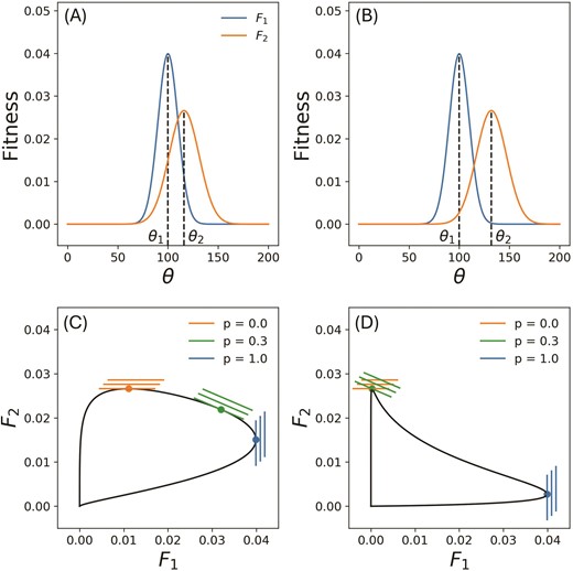
(a,b) Fitness functions and of an organism subject to two distinct environments and . The fitness is assumed to have a Gaussian form over the range of available phenotypes , with its maximum value at the optimum , and width , a measure of the selection pressure. We have , and in both (a) and (b), whereas changes from 116 in (a) to 132 in (b). The fitness set corresponding to (a) is shown in (c). Since the optimal phenotypes of the two environments are close and the fitness functions and have considerable overlap, the fitness set in convex. In contrast, for (b), where the two environmental optima are farther apart, the corresponding fitness set (d) is concave. (c,d) also illustrate the family of adaptive functions defined in Equation 2 for and 1.0. Here p is the frequency with which the organism encounters environment . The optimal phenotype for a given p value is the point where the corresponding adaptive function intersects the fitness set with the largest intercept A. In (c,d), the orange and blue set of adaptive functions pick out the optima of the two corresponding environments shown in (a,b).
Thus, is the optimal phenotype that maximizes fitness in environment , and characterizes the strength of selection pressure in the environment. We make the assumption here that the area under each fitness curve remains constant. Less selective environments have higher values and lower peaks ( in Figure 1(a,b)), and allow for a broader range of phenotypes of comparable fitnesses. In contrast, highly selective environments only support a narrow range of phenotypes, and have low values and higher peaks ( in Figure 1(a,b)). However, when this assumption is relaxed, and the height of our fitness functions is allowed to vary independently of its width, we find that the main qualitative results of our study hold. This is shown in Section S6, Figure S7 in Supplementary Information.
We will consider the case where these environments are dynamic, such that the optimal phenotype change with respect to time (Figure 1(b)), whereas the width of the fitness functions remain constant. This makes our approach parallel to the classic model of adaptation to an environment with a gradually shifting optimum Lande (1993); Bürger & Lynch (1995). When subject to both environments simultaneously, the optimal phenotype can be different from both the optimal phenotypes, and also changes with time, although not linearly.
The fitness set is the parametric curve in between and , and each point on it represents an individual or a monomorphic population with a distinct phenotype (Figure 1(c,d)). The optimal phenotypes corresponds to the point on the fitness set with the maximum value of . A straight line joining two points A and B on the fitness set, represents a polymorphic population that has a mixture of the phenotypes corresponding to A and B. The fitness set is convex when and are close to each other in fitness space, or in other words, when the overlap between the fitness curves and is large (Figure 1(c)). When this overlap decreases, the fitness set becomes concave (Figure 1(d)). The shape of the fitness set changes as either of the environmental optima changes, becoming more concave as the distance between the two optima increases. Thus, the concavity of the fitness set is a measure of the strength of the trade-off between performance in the two environments.
In order to determine the optimal phenotype for the combination of the two environments, we need further information about the distribution of environmental heterogeneity. The distribution of the heterogeneity determines the form of the effective total fitness function. This is given by the adaptive function, which encodes information about the frequency with which the organism is subject to selection pressure from a particular environment. We will restrict our study to the case of a linear adaptive function of the form
where is the frequency with which the organism encounters environment . The linear adaptive function captures cases of ‘fine’ heterogeneity, where patch size of each environment (in time or space) is small. The population should be able to access both environments at time scales much shorter than the generation time for the linear equation to hold. For a derivation of the same, see Levins (1968). The other extreme alternative, where population individuals must make a decision between the two environments, or can only access one or the other at time scales comparable to the generation time can be described by a hyperbolic adaptation function Levins (1968). Intermediate patch sizes can be described by interpolating functional forms between the linear and hyperbolic functions.
The linear adaptive function represents a family of straight lines in fitness space which have slopes (Figure 1(c,d)). The optimal phenotype is defined to be the point on the fitness set that intersects the line at the largest possible value of . Note that points within the fitness set have lower fitness than those on it, and all points outside of the fitness set are unachievable. Thus, the optimal phenotype calculated in this manner both maximizes total fitness, as well as satisfies the constraint from the trade off between the two environments. For a more detailed exploration of the method, see Levins (1968). For (), only the second (first) environment is experienced by the population and the optimal phenotype is a specialist that is maximally adapted to the second (first) environment, i.e., it is identical to (). For ; however, the optimal phenotype depends on the curvature of the fitness set. When the fitness set is convex, the optimal phenotype could also be a generalist, which is not optimally adapted to either environment but performs moderately in both (Figure 1(c)). If the fitness set is concave, however, the only optimal strategy is a specialist, either adapted to the first or the second environment depending to the value of (Figure 1(d)). Note that since we are considering a fine distribution of environmental heterogeneity, the possibility of mixed population of the two specialists or bet hedging is always less optimal than the generalist solution in case of a convex fitness set and less optimal than a specialist strategy in case of a concave fitness set. The bet-hedging strategy becomes more fit as the effective patch size becomes larger.
For the purposes of this paper, we will assume that only the second environment changes in time. We do this for the sake of simplicity, but also to be able to compare our results with previous studies that consider adaptation to a single linearly changing environment Lande (1993); Bürger & Lynch (1995). Thus, while remains fixed, evolves dynamically as , where is the rate of change of the environment with respect to the generation time, . The optimal phenotype can be calculated for a particular pair numerically, using a solver which locates the value of for which the slope of the fitness set () is identical to slope of an adaptive function (Eq. 2) with the highest value of for a given . As the two specialists move farther apart from each other in fitness space, the fitness set goes from being convex to concave (Figure 2(a,b)), and the optimal phenotype for switches from a generalist to a specialist (Figure 2(d,e,f)). As can be seen in the figure, the shift can be sudden or gradual with respect to the generation time depending on the value of and the asymmetry of the fitness set given by (). We find that even for a linearly changing environment, its combination with a second static environment means that changes in the optimal phenotype are not only non-linear but can also be non-monotonic. For high enough values of the optimal phenotype returns close to its original value by switching to the specialist of stationary environment . Lower values of cause the optimum to switch to the changing specialist in . This occurs after a period of non linear change as a generalist. This is distinct from the case of adaptation to a single environment where the change in the optimal strategy is linear throughout the course of evolution Lande (1993); Bürger & Lynch (1995); Chevin et al. (2010). As we will see, the non-linear portion of the optimal strategy curve with respect to time has the potential to change the probability of extinction events in adapting populations.
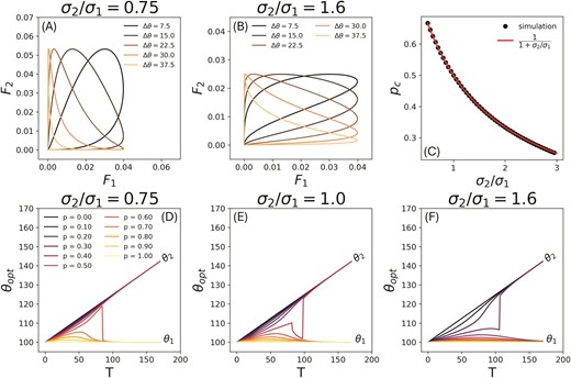
(a,b) Fitness sets at different times for and , respectively, as the optimum of one environment moves away from the other. In both cases, and the specialist changes with time T as with , while remains constant at 100. As increases, the fitness set in both cases goes from being convex to concave. (c) The critical value . For p values below , the long term optimal strategy is the stationary optimum. The values were obtained numerically by implementing a binary search algorithm (see Section S2 of Supplementary Information) in the range to identify up to 4 digits of precision the value of p above which the optimal phenotype switches from the moving to the stationary optimum at long times. The critical value is independent of v and only depends on , and simulation results show excellent agreement with the analytical prediction in Equation 3. Note that the form of is dependent on our assumption that the area under the fitness curves remains conserved. When this assumption is relaxed, ceases to depend on . This is shown in Section S6, Figure S7 (d) of Supplementary Information. (d,e,f) The optimal phenotype with respect to time for different values of p (the frequency with which the stationary environment is encountered), and for , and , respectively. For a given set of parameters , the optimal phenotype as a function of time T was calculated by numerically solving for the point on the corresponding fitness set that is intersected by the adaptive function with the highest possible value of . In all three cases, , , and .
Which of the two specialists is picked as the long-time specialist strategy depends on both , as well as the ratio of the environmental selection strengths . As increases, the second environment becomes less selective and the concave fitness set goes from being rounded near the second environment’s optimal and sharp near the optimal phenotype of the first environment, to being sharp near the second optimal and rounded near the first optimal phenotype. There is a critical value such that the long-time optimal strategy is a specialist adapted to the stationary niche for , and a specialist equivalent in the moving environment for . This critical value of can be shown (see Supplementary Information section S1) to depend on the asymmetry as
As shown in Figure 2(c) this analytical form shows agreement with numerically evaluated values of as a function of . Note that the dependence of on arises from our assumption that the height and width of the fitness functions cannot be changed independent of each other, since the area under the fitness function remains preserved. Once this assumption is relaxed, ceases to depend on . This is shown in Sec. S6, Figure S7 (d) of Supplementary Information.
Individual-based population level simulations
We have seen the trends possible in the optimal phenotype for a system with two environments, one of which shows long term change. We can now ask how a population would respond to selection from such a combination of environmental cues. How different will its behavior be from a population adapting to a single linearly changing environment? Consider an asexually reproducing population with discrete, non-overlapping generations. As before, we assume that an individual’s fitness in the population can be captured by a single phenotypic quantity, . The population is made up of individuals with phenotypic values that are drawn initially from a normal distribution in . This phenotypic trait is under selection from the optimal phenotype derived for the two environments.
We assume that the population is initially at mutation-selection balance. This means that the spreading effect of mutations is countered exactly by the contracting effect of selection on the population. If there are no dynamic changes in the two environments, both the mean and standard deviation of the population remains preserved in time. We start the population then with a mean at the initial effective optimal phenotype and the population variance is given by
where is the variance of mutation effects for the population. The derivation of this population standard deviation is given in Sec. S1 of Supplementary Information. At every generation we calculate the fitness of each member of the population according to their individual phenotype and its distance from the optimal phenotype. An effective Gaussian fitness function is used with its optimum at the effective optimal phenotype calculated using the method described in the previous section. We take the following form for the width of the effective fitness function, or the effective strength of selection,
Note that the width of the weighted sum of two Gaussians includes generally a contribution from the difference in their mean values. For our calculation of the effective variance, this quantity would change with time as one environment moves away from the other. We chose to make a simplifying assumption here and ignore the time dependent contribution to the effective width. The contribution from the means of the fitness functions has a prefactor and is of an order lower than the contributions from the widths of the fitness functions. Upon relaxing this assumption and including the time-varying term in the effective width, our results remain qualitatively preserved. This is shown in Sec. S7 of Supplementary Information.
The fitness of each individual is then used to calculate the number of offspring for each individual. The maximum possible number of offspring, or the maximum fecundity of an individual is given by . The number of offspring for each individual is then given by , where is the individual’s phenotype and is a Gaussian fitness function of the phenotype with its optimum at the effective optimum , and width , . The phenotypic distribution for the next generation of individuals is determined by assigning each offspring the phenotype of its parent plus a small beneficial or detrimental mutational fitness increment, drawn from a normal distribution with zero mean and standard deviation equal to , which sets the mutational standard deviation in our model. We are thus assuming that the phenotypic trait is polygenic and that mutations with small fitness changes are much more likely to occur than large effect mutations. We also assume that there is no contribution to the phenotype from environmental variation, and it is entirely determined by the genotype.
The population undergoes growth in successive generations such that the total number of individuals in the population is restricted to a carrying capacity, . The simulations are started with a population that has individuals. After each cycle of selection, if the number of individuals in the new generation exceed the carrying capacity, the population is reduced again to by randomly selecting individuals. If the number of individuals in the new generation is equal to or less than , the entire population in retained. The mutation process as well as random selection of offspring at every generation makes our simulation stochastic.
We study the dynamics of the population by keeping track of its mean, its phenotypic variation and the size of its offspring population after density dependent regulation. We find that the survival probability, phenotypic lag and mean time to extinction of the population depends crucially on the relative frequencies of the environments in addition to other environmental parameters like rate of change, population parameters like carrying capacity and maximum fecundity as well as the mutational standard deviation.
Results
We will first summarise the various population level trends we see in our simulations, and then analyse their dependence on the different parameters of our model. For populations that have , the long-time transition of the optimal phenotype to the static specialist means that the optimal phenotype now remains fixed despite a change in the other environment. This is a strategy for probable survival. However, the population remains maladapted to the moving environment in which the birth rate is effectively zero. Thus the population faces a demographic load due to the moving environment acting as a sink, sustained only by the production in the stationary environment Pulliam (1988); Ronce & Kirkpatrick (2001). The population experiences an average fitness of . The population needs to be productive enough in the stationary environment such that even though the effective fitness is lowered by a factor compared to a population that only experiences a single stationary environment, it can sustain this demographic load. For the population to survive, then, it would have to satisfy . For the demographic load is small enough for our survival probabilities to hold for all . For the cases where , the demographic load would change survival probabilities, since we do not explicitly include this demographic load in our calculations. In either case, a higher can allow the population to deal with the demographic load of being a specialist in a heterogeneous environment. Population survival can be seen for all in Figure 3 (a), where we consider a case with equal environmental selection strengths.
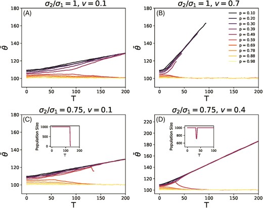
Mean phenotype of the population as a function of time from results of simulations of the evolution process for in (a) and (b), for (c) and (d). These are plots for a single replicate population. In (a) is a plot for rate of change , and (b) is a plot for . Plot (b) shows several extinction events for the populations that are undergoing adaptation to the moving environment’s specialist, implying the existence of an upper bound on rate of change for population survival. In (c) is a plot for , and in (d) is a plot for . The insets show the population size as a function of time. Plot (d) shows the population corresponding to survive though it goes extinct at a lower rate in (c), implying the existence of a lower bound on rate of change for population survival. The inset on the right shows a process of evolutionary rescue. For these plots , , , , and .
For populations with that change from a generalist to a specialist adapted to the moving environment, the problem is similar to that of a population adapting to a single changing environment. However, the initial period of non-linear change when the optimal strategy is a generalist means that the population is not at mutation-selection balance when it enters the following phase of linear change. Further, the population faces an additional demographic load from maladaptation to the second environment, and the second environment acts as a sink. Large enough populations survive at low enough rates of change, and follow the optimal phenotype. This can be seen in Figure 3(a,b) where (a) shows all populations surviving, whereas at a higher rate of change, shown in (b), all populations that face selection from the moving environment go extinct. The dependence of population survival on the population size is captured in Section S4, Figure S5 of Supplementary Information, which shows the variation of the critical rate of change with . We define the critical rate of change and explain its relevance in Section 3.1. It is important to note that the non-linearity in the evolution of the optimal phenotype with time, which is the consequence of a trade-off with the stationary environment, allows for higher critical rates of change for the shifting environment. We explore the critical rate of change below which populations are likely to survive in Section 3.1. For the populations that survive with , we find that the mean phenotype follows the optimal phenotype with a phenotypic lag in an equilibrium state. The value of this lag is significant since larger lag implies higher selection pressures and smaller population sizes, that make the population more vulnerable to stochastic extinction events Beissinger (2000); Flather et al. (2011); Lynch et al. (1995). We will explore the magnitude of phenotypic lag more in Section 3.2.
Surprisingly, for , the populations that go extinct the fastest, as shown in Figure 3 (b), are not the ones with lowest , i.e. the ones that rely the most on the changing environment, but the populations with values close to but lower than . This is because the survival of populations that try to adapt to the moving optimum also depends on the number of generations for which the optimal phenotype is a generalist. This is highest for those populations with values adjacent to . In general, for an arbitrary , the populations close to are most vulnerable, because they involve the largest abrupt changes from the generalist to a specialist phenotype.
Further, survival depends on how sudden the shift from the generalist to the specialist is compared to the generation time. For asymmetric selection strengths (), we observe instances of abrupt and large non-monotonic change in the optimal phenotype (Figure 2(c,e)). In such cases, even where , survival depends on the duration of change away from the stationary optimum preceding the return to it, during which the population adapts away from its eventual equilibrium specialist optimum. Thus, the faster the change of the optimal phenotype to the stationary environment, the higher is the chance of survival for the population. This leads to the counter-intuitive phenomenon of a lower bound on the rate of change. Below this critical rate the populations face extinction, and above it survival is possible. This is shown in Figure 3 (c) where at a rate of the population corresponding to goes extinct and the population size plummets to zero. Upon increasing the rate of change to in Figure 3 (d) the population shows a case of successful evolutionary rescue as can be seen in the population size plot. This kind of behavior is only seen in a narrow range of values close to , and we will explore this more in Section 3.1 for different values of asymmetry.
Thus, we observe that the addition of a secondary environment not only introduces a dependence on , i.e. the frequency of the two environments, but also changes the dynamics of extinction and survival in surprising ways. In the next subsections we will look more closely at parameter regimes where populations tend to go extinct, and explore the phenotypic lag in cases where the population survives.
Bounds on rate of change, extinction, and survival
Previous work has shown that in linearly changing environments a critical rate of change exists above which populations go extinct in deterministic models. The value of this critical rate depends on selection strength, the fecundity of the population and the available phenotypic variation Lande (1993); Bürger & Lynch (1995). Since our model is stochastic, we look at the probability of survival for a certain parameter regime. We run the simulation over different populations to generate probabilities.
Figure 4 shows the probability of survival for a population for different values at varying rates of change and asymmetry in environmental width. In (b–f), the boundary between the yellow and blue regions in the plots represents the critical rate of change for populations at each value of . As expected in our model, for , the population almost always survives once it lapses to the stationary optimal phenotype. As stated, the additional effect of maladaptation to the moving environment should be considered on these survival probabilities.
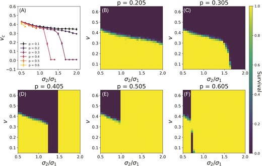
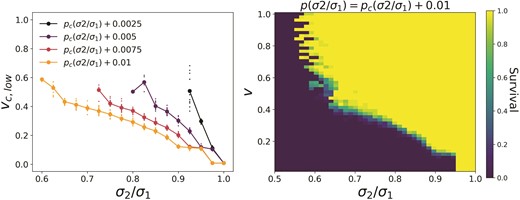
Critical rates of environmental change. (a) Upper bound on the rate of change as a function of with and mutational standard deviation 0.5, averaged over 25 initial populations. We only report for values of at which populations go extinct above this critical rate. Cases of where the population survives for all values of v are not plotted here. (b-f) Probability of survival over 25 runs of the population dynamics for different values of rate of change and . The yellow regions are areas where all populations survived, and blue are where they all went extinct. The boundary between the two represents the two critical rates. The lower critical rate only exists in the panel for . For these plots and .
Upper bound on rate of change
Let be the critical rate above which populations go extinct if they are adapting to the moving environmental specialist. As can be seen from Figure 4(a), and from the boundaries of Figure 4(b-f), for , decreases monotonically as increases. Here we change by keeping fixed and varying . Note that this trend is similar to models of adaptation to a single moving optimum, where weakening selection from the moving environment causes the critical rate of change to decrease.
In addition to a dependence of on parameters of the single moving optimum models, we also see a dependence on and together. At middle range values of , like can be seen in and there is a range of where populations do not survive for any rate of change ( for and for ). For at these asymmetric environmental widths, the fitness set is skewed and the optimal phenotype as it evolves in time, exhibits sudden jumps that cause the population to crash. When is greater than the value for a given , all populations are able to survive even for high rates of changes, by losing their dependence on the moving environment and adapting to the stationary optimum. The critical rate of change of the environmental optimum increases with fecundity, eventually saturating. This is shown in Sec. S4, Figure S3 of Supplementary Information. Increasing the mutational standard deviation also increases the critical rate of change by allowing for faster adaptation, as is shown in Sec. S4, Figure S4 of Supplementary Information. Lastly, increasing causes to increase due to reduced stochasticity from a larger population size. For more on how varies with carrying capacity see Sec. S4, Figure S5 in Supplementary Information.
Lower bound on rate of change
The plot for in Figure 4 shows a small regime of extinction around which is bounded from above in by an area of survival. This region is an example of the existence of a lower bound in rate of change for survival, which can occur only for systems where and just above .
The lower bound reflects the fact that a population is more likely to survive if the time spent as a generalist is shorter such that fewer generations of the population adapt away from the final specialist phenotype. This only occurs at values that are slightly larger than when .
We explore this in Figure 5 by varying and together such that , where is a small offset in from its critical value. The left plot shows the lower critical rate, for different values of at a few different values of . The right plot shows the probability of survival for .
Lower bound on the rate of change. Both plots vary p and together such that . The left side shows the lower critical rate, for different , with the bigger points depicting the average over 25 populations, and the smaller points showing the spread around this average. The right plot shows the probability of population survival for . Here, and .
It should be noted that the lower bound and upper bound on the rate of change are seen in exclusive parameter regimes. This can be seen in Figure 4. For populations where we see the existence of , populations above always survive since they adapt to the specialist of the stationary environment. Note that this is a novel phenomenon which is not seen in models that consider adaptation to a single environment. Such models only allow for the possibility of linear change in the optimal strategy, and thus only an upper bound on the rate of environmental change exists Chevin et al. (2010).
Phenotypic lag
For populations with , survival depends in a complex way on the rate of change of the environment, as well as the asymmetry in the selection strengths of the two environments. For the populations that do survive, we observe that an equilibrium state is reached where the mean of the population changes linearly with time, following the optimal phenotype of the changing environment. This is true for the populations that survive in Figure 3 (d), where all the populations that survive for lower values converge on to the moving optimum. The process of adaptation for these populations is similar to that for a population adapting to a single environment whose optimum changes linearly with time, even though survival probabilities are different because of the non-linear generalist phase of the optimal phenotype. Supplementary Information Sec. S3, Figure S2 shows the equilibrium mean phenotypic lag and standard deviation of populations that evolve to the two specialist phenotypes.
Figure 6 shows the value of the phenotypic lag in our simulation for different values . The smaller points show the individual populations that survive, whereas the larger points show the mean. For surviving populations, lag is zero when the population chooses the stationary optimum. For populations that follow moving specialist the lag increases as increases along the axis. This is because the selection strength is lower for higher . As expected, the lag is largest for values close to , represented by the points right before lag falls to zero when the stationary optimal phenotype is chosen as a specialist since these populations spend the most time in the non-linear phase before reaching equilibrium. This is significant since the lag of the population in equilibrium is an indication of the fitness of the population. The higher the lag, the lower the population fitness. Population size is lower for populations that have a lower fitness at equilibrium, making populations more vulnerable to stochastic extinction events. This explains why we see populations with values close to but higher than go extinct first. Unsurprisingly, the lag increases faster at higher rates of change than at lower rates.
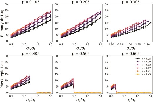
Phenotypic lag for different values of and different rates of change v. The smaller points represent the lag for individual populations and show the spread around the mean, which is represented by the larger points. Only populations that survive the entirety of the simulation are represented here. Lag increases with asymmetry in the environmental widths. The lag is measured at the final equilibrium by taking the average of many time points after equilibrium has been reached. For these plots and .
Mean time to extinction
For populations that go extinct, we look at the mean time to extinction. The bold points in Figure 7 (a,d) show the mean time to extinction at different and values, while the smaller points show the extinction times for individual population replicates. Figure 7 (b,c,e,f) shows the optimal phenotype (dashed) and the mean phenotype (solid) of one adapting population as a function of time for different values of and , and the colors depict the environmental asymmetry . Populations that survive till the end of our simulation are not shown here.
We find that, although in all cases the mean time to extinction decreases with increasing rates of environmental change , there are in fact two kinds of extinction events that can occur, depending on the value of relative to a critical asymmetry for each value of (Figure 7(a,d)). We define to be this critical value of for a particular value of . For , extinction is driven by the phenotypic lag with respect to the optimum, as is clear in Figure 7 (b,c,e,f) from the curves in the blue end of the spectrum of the colorbar for . In this regime of extinction, the mean time to extinction decreases as the lag increases with increasing (below ), and the moving environment becomes less selective. However, the rate of this decreases becomes smaller or even zero for higher values of , for which populations lag behind the optimal phenotype from very early stages of adaptation, and thus have a reduced dependence on how the environmental asymmetry affect phenotypic lag.
For however, extinction is driven by large abrupt changes in the optimum from the vicinity of the stationary to the moving specialist. This is again confirmed in Figure 7 (b,c,e,f) by the curves in the yellow end of the spectrum. Since extinction is now determined almost entirely by the time of the abrupt switch in the optimum (which increases with increasing ), the mean time to extinction also increases correspondingly for all values . Note that there is no spread around the mean value for extinction time because the time of extinction is determined almost exactly by the time at which the optimum makes its abrupt switch.
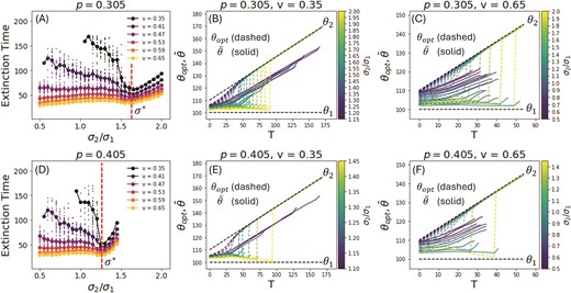
Time to extinction for different values of and different rates of change v. In (a,d) the smaller points represent the time to extinction for individual populations and show the spread around the mean, which is represented by the larger points. Populations that survive the entirety of the simulation are not represented here. In (b,c,e,f), we plot the optimal phenotype (dashed) and the mean phenotype (solid) of a population adapting to this optimal phenotype as a function of time T, and for different values of the asymmetry (colorbar). For all p and , increasing the rate of environmental change v leads to a decrease in the mean time to extinction. At a particular p dependent value of the asymmetry the curves in (a) and (d) show a minimum in the extinction time, marking two different regimes of extinction events. Below( extinction is driven by the lag with respect to the optimal phenotype, as can be seen from the curves in the blue end of the spectrum in (b,c,e,f). The lag increases as increases, leading to a decrease in the mean time to extinction for low v, and fairly constant extinction times for high v in this regime. Above extinction is almost entirely determined by the time at which the optimum has a large abrupt shift from the stationary to the moving specialist. This time increases with increasing , resulting in a corresponding increase in the mean time to extinction in this regime. For these plots and .
Discussion
We have demonstrated that adaptation to long term environmental change in the presence of multiple environments with trade offs is qualitatively different from evolution in a single changing environment. We find certain novel phenomena that arise with the combination of heterogeneity and long term environmental shifts. First, even when the environmental change is linear and unidirectional, the optimal phenotype of the population may show non-linear and even non-monotonic behavior over several generations. Large changes in the optimal phenotype that are sudden compared to the generation time become possible. When one of the environments is stationary, this can lead to the existence of a counter-intuitive lower bound on the environment’s rate of change, such that below this rate populations go extinct, while above it they survive. This is because when the long-term optimal strategy is a specialist suited to the stationary environment, it is more beneficial for the population to have a shorter generalist phase of non-linear change in the optimal phenotype, such that they spend fewer generations evolving away from the stationary optimum.
This behavior is seen in a narrow range of parameters and for environments that have different widths. We also find the existence of an effective upper bound on the rate of change of the environment above which populations go extinct for adaptation, which is also seen in the case of a single linearly changing environment Lande (1993); Bürger & Lynch (1995); Chevin et al. (2010).
We recognise that the lower bound on the rate of change is a very specific phenomenon that occurs in a narrow parameter regime, yet it points to the possibilities of non-monotonic behavior in the optimal phenotype when multiple environments are involved. We see the importance of this behavior as a qualitative indicator of novel and interesting behavior that may occur in complex real world populations.
Non-linear changes in the optimal phenotype have been addressed in models before Osmond & Klausmeier (2017); Schluter (1988). These studies point out that the critical rate of environmental change considered in quantitative genetic models depends on the form chosen for the fitness function. For fitness functions that show weakening selection with phenotypic lag ( or non-quadratic fitness functions), inflection points can cause population growth rates to drop from positive to negative. There has also been an attempt to extend earlier results to include the possibility of the height fitness function of the moving environment decreasing with time Klausmeier et al. (2020). Both these cases show the possibility of sudden changes in the optimal phenotype despite a smoothly changing environment, similar to the sudden shift we see here from generalist to specialist optimum phenotypes. It should be noted, however, that the nonlinearity in the optimum in our model is independent of the form of the fitness function (since any transition of the optimal strategy from a generalist to a specialist will cause non-linearity) and is a result of the two time scales of change considered together. Having said that, taken together, these results point to the possibility that complex ecological interactions will cause adaptation to long term change to include adaptation to sudden changes in the optimal phenotype.
Further, we find a crucial dependence of population survival and extinction on the relative frequency of the two environments, . We find that there exists a critical value for each value of , below which the population loses its dependence on the changing environment. For such populations the changing environment acts as a demographic sink, and they can survive long term environmental shifts only if they produce enough offspring in the stationary environment. We do not explicitly include this phenomena in the calculation of survival probabilities. Hence we see populations of specialists in the stationary environment survive almost all of the time. The probability of survival for populations that have have long term optimum fitness at the stationary optimum could be studied using a model similar to those in Ronce & Kirkpatrick (2001); Pulliam (1988). It should be noted however, that for , the demographic load is small enough for our survival probabilities to hold for all . For the cases where , the demographic load would change survival probabilities. In either case, a higher can allow the population to deal with the demographic load of being a specialist in a heterogeneous environment, since to survive the population must satisfy .
For populations that do adapt to the moving environment, we see the possibility of two kinds of extinction events, in contrast to studies with a single changing environment Bürger & Lynch (1995); Lande (1993). The first kind is driven by the phenotypic lag behind the optimal strategy and is thus intensified by a decrease in the selection strength of the moving environment for low rates of environmental change. Above a certain dependent value of the selection strength however, we see another kind of extinction driven by a large and abrupt switch in the optimal phenotype from the vicinity of the stationary to the moving specialist. This second kind of extinction is predominant for values close to and below , for which populations spend many generations adapting to a generalist phenotype that is closer to the stationary optimum, before a specialist corresponding in the moving environment suddenly becomes more optimally fit. This means that for environments with similar selective strengths, the populations that are most vulnerable are those that depend on several environments with similar proportions.
The framework of fitness sets is a useful tool in studying adaptation in complex and dynamic environments and deserves more attention. The framework allows for a quantification of trade off strength and its relationship to phenotypic diversity, much like is emphasized in recent papers that use the Pareto front to talk about niche construction and diversity Sheftel et al. (2013); Shoval et al. (2012). However, in addition to this, the adaptive function also allows for a characterization of the distribution of environmental heterogeneity. It allows for a discussion of both spatial and temporal heterogeneity in the same framework.
We also examine the effects of relaxing our assumptions, by allowing the fitness functions to have heights independent of their widths (in Sec. S6 of Supplementary Information) and of including a time dependent term arising from the difference in optima in the effective width (Sec. S7 of Supplementary Information). We find that the existence of both lower and upper bounds are robust to these changes in assumptions. The fact that a more complicated fitness function (width depending on the distance between the means) qualitatively reproduces our results suggests that the generality of this framework, and the conclusions that can be drawn from it, are robust to changes in mathematical detail. Further, for any functional form of the fitness functions, there will always be a critical value of at which the transition for the long term choice of specialist occurs. As long as there exists such a value , we expect all of our results to hold qualitatively. The phenomenon of the lower bound is tied to the existence of , and the upper bound has been shown to exist for different functional forms of fitness.
The results of our model apply to ‘well mixed’ or ‘fine’ cases of heterogeneity, where the time scales at which the population encounters the two environments is much smaller than the generation time. This assumption is why we observe the collapse on to a stationary niche as the optimal strategy for a range of values. Future work could address the more general case of heterogeneity that is ’coarse’, where environments present more as discrete choices to the population, or change at time scales comparable to the generation time. In this case, the adaptive function would take on a non-linear or hyperbolic form. Bet hedging, or populations of mixed specialists then become optimal for a range of values. This would lead to the interesting phenomenon where a population of generalists undergoes selection from two diverging environmental optima to produce a mixed populations of specialists. This could be harnessed to examine the possibility of increased specialization, and perhaps even speciation, from selection under climate change Bridle et al. (2014); Berlocher & Feder (2002); Bolnick and Fitzpatrick (2007). Additionally, more complexity can be added to our model by allowing both environments to shift. The simplest case of this where both environmental optima shift in opposite directions at the same rate is briefly explored in Sec. S5, Figure S6 of Supplementary Information.
Incorporating phenotypic plasticity into our model, which may change the boundaries between survival and extinction, is the scope of future work Lande (2009). The effect of phenotypic plasticity would manifest in different ways at the two time scales we are considering. As Levins pointed out, at the level of heterogeneity, plasticity may increase fitness in both environments simultaneously, causing the fitness set to become more convex and reducing the effective strength of the trade off Levins (1963). At the level of dynamics the presence of phenotypic plasticity may have a two competing effects. Plasticity may aid in cases of evolutionary rescue by reducing the effective rate of change of the environment that is moving Chevin et al. (2010). On the other hand, by quickening adaptation away from the stationary optimum, phenotypic plasticity may worsen chances of survival for populations adapting to a non-monotonic optimal phenotype.
For our study, we assume that the fitness can be described entirely by the environmental optimum and a single phenotype. If we were to consider multiple phenotypes, we would have to consider the effect of correlations and trade-offs between phenotypes arising from the genotype to phenotype map.
We have considered an asexually reproducing population and assumed that mutations in offspring cause a small change in the phenotype in question. Since our model does not include an explicit genotype to phenotype map, examining the effect of sexual reproduction and recombination on our results is outside the scope of this study. We expect, however, that sexual reproduction could have an effect similar to increasing the variance of the distribution of phenotypic effects of mutations Charlesworth (1993); Bürger (1999); Waxman & Peck (1999). A higher mutational standard deviation leads to faster adaptation in our model, leading to higher survival probabilities. There is some evidence in the literature to suggest that sexual reproduction can facilitate adaptation to new environments Becks & Agrawal (2012); Goddard et al. (2005).
The results of our model can be verified by long term studies that keep track of population level phenotypic distributions. Systems that have a combination of short term variation with long term environmental change are common in climate change studies. Such studies in marine systems show that organisms must adapt to multiple stressors such as acidification and temperature changes, and that their evolution is different from evolution in response to one stressor Kelly et al. (2016); Brennan et al. (2022); Kelly & Griffiths (2021); Gerhard et al. (2023). Such a system can also be set up with laboratory evolution of yeast or bacteria. Fluctuations in food resource or temperature could be simple examples. Some studies have hinted at the lack of trade-offs in bacterial systems that evolve to different temperatures, arguing that trade-offs may not be universal Bennett & Lenski (2007); Velicer & Lenski (1999); Bono et al. (2017). However, a method of determining specialists and their associated phenotypic traits, like has been used for generating Pareto fronts from ecological and high dimensional gene expression data, may allow for the discovery of true trade-offs Shoval et al. (2012); Hart et al. (2015). Bacterial and yeast systems also carry the advantage of a short generation time.
Several experiments show resonance with our results. The existence of an upper bound on the rate of change has been observed in marine systems such as plankton Lynch et al. (1991). The lower bound on the rate of environmental change in our model can be related to experimental and theoretical studies of evolutionary rescue in populations which show that while slow changes can generate more effective growth in extreme environments at short time-scales, it comes at the cost of a lower probability of long-term survival Liukkonen et al. (2021); Uecker et al. (2014). Further, the lapse on to the stationary optimum that we observe is reminiscent of adaptation through gene loss that is seen in bacterial populations, which is contrary to the notion that adaptation is the development of additional ability and complexity Hottes et al. (2013); Morris et al. (2012). Loss of function as an adaptive strategy has also been seen in plants adapting to stressors and novel environments Monroe et al. (2018); Dong et al. (2021). However, most studies on loss of function are at the level of genetic data, making a direct comparison with our results difficult. For a full evaluation of our results, more long term studies in the spirit of the 30 year long study of the Galagapos finches, that carefully document phenotypic distributions as well as environmental variation would be required Grant & Grant (2002).
Supplementary material
Supplementary material is available online at Evolution.
Data availability
The code used to generate the simulation results in the paper is available at https://github.com/purbachat/Phenotypic_Adaptation_Levins.
Author contribution
N. Chaturvedi and P. Chatterjee conceptualised the problem, ran simulations and wrote the manuscript.
Funding
N. Chaturvedi was supported by the Simons Foundation (287975).
Conflict of interest: The authors declare no conflict of interest.
Acknowledgments
We thank Mukund Thattai and Archishman Raju for helpful discussions.
