Quantitative assessment of observed versus predicted responses to selection

Abstract

Although artificial-selection experiments seem well suited to testing our ability to predict evolution, the correspondence between predicted and observed responses is often ambiguous due to the lack of uncertainty estimates. We present equations for assessing prediction error in direct and indirect responses to selection that integrate uncertainty in genetic parameters used for prediction and sampling effects during selection. Using these, we analyzed a selection experiment on floral traits replicated in two taxa of the Dalechampia scandens (Euphorbiaceae) species complex for which G-matrices were obtained from a diallel breeding design. After four episodes of bidirectional selection, direct and indirect responses remained within wide prediction intervals, but appeared different from the predictions. Combined analyses with structural-equation models confirmed that responses were asymmetrical and lower than predicted in both species. We show that genetic drift is likely to be a dominant source of uncertainty in typically-dimensioned selection experiments in plants and a major obstacle to predicting short-term evolutionary trajectories.

breeder's equation, evolvability, G-matrix, indirect selection, Lande equation, correlated traits, artificial selection, Dalechampia

At the core of evolutionary quantitative genetics sits the Lande equation, which predicts the mean evolutionary response of a set of characters as the product between the selection gradient and the additive genetic variance matrix, G (Lande 1979; Lande and Arnold 1983). Many studies have confirmed that the geometry of G influences the response to selection (e.g. Hine et al. 2014), and patterns of population and species divergence in multivariate character space are often congruent with directions of high evolvability in G (e.g., Schluter 1996; Hansen and Houle 2008; Bolstad et al. 2014; Houle et al. 2017; McGlothlin et al. 2018; Hansen and Pélabon 2021). The realization that evolutionary changes are important at ecological time scales (Kopp and Matuszewski 2014; Reznick et al. 2019) and the subsequent development of the eco-evolutionary dynamics (Hendry 2017) underscore the relevance of quantitative genetics theory to microevolution beyond animal and plant breeding. The utility of quantitative genetics to ecology and management rests on its ability to predict short-term evolution, however, and both empirical and theoretical studies have cast doubt on whether sufficient accuracy can be expected to allow meaningful forecasting in specific cases (e.g., Hansen et al. 2019; Shaw 2019; and see Hendry 2017, chapter 3 for a review of the performance of the Lande equation in predicting short-term evolution in natural populations).

The breeder's equation also has somewhat mixed performance in predicting the outcome of univariate selection experiments in the lab (Sheridan 1988; Eisen 2005; Walsh and Lynch 2018, chapter 18), and its success in predicting correlated responses in traits under indirect selection is generally considered to be poor (e.g., Bohren et al. 1966; Rutledge et al. 1973; Palmer and Dingle 1986; Gromko et al. 1991, 1995; Cortese et al. 2002; Roff 2007). This is a serious concern, because indirect selection may well be the major component of selection on most traits in natural populations. The main advance brought by the G-matrix was the ability to predict correlated responses, and if this cannot be done reliably, then inferences about genetic constraint based on G must be poor.

Most assessments of evolutionary predictions have been qualitative, however, and when prediction uncertainties are presented, they are usually given as estimation errors in realized heritabilities based on very simple models of the underlying genetic architecture, and further reduced to statements about “significant” difference between predictions and observations (e.g., Hill and Caballero 1992; Walsh and Lynch 2018, chap. 18). For correlated responses, uncertainties have almost never been presented, and claims of poor prediction of correlated responses are based largely on qualitative assessments (e.g., Roff 2007).

There are three main sources of error in predicting evolutionary responses: (i) errors due to discrepancies between the model used for prediction and the actual evolutionary process; (ii) errors made in estimating the parameters in the chosen prediction model, and (iii) errors due to inherent stochasticity in the response.

Deterministic discrepancies from simple predictive models such as the Lande or breeder's equation are unlikely to be substantial in the first few generations, but as selection extends over more generations, the response may deviate due to a number of issues related to details of genetic architecture, inbreeding and counteracting natural selection (Le Rouzic et al. 2011). In principle, more detailed models can be fitted to evolutionary time series to estimate parameters describing such effects (e.g., Le Rouzic et al. 2010, 2011; Walsh and Lynch 2018, chapter 19), but this has rarely been done.

Various methods have been suggested to assess the effects of sampling error in quantitative genetic parameters on prediction variance (Tai 1979; Knapp et al. 1989; McCulloch et al. 1996; Conner et al. 2011). Stinchcombe et al. (2014) used a Bayesian approach and combined the Price equation with the Lande equation to estimate uncertainties of the predicted response to a single generation of selection from the posterior distribution of the G-matrix and the selection gradients (see also Careau et al. 2015).

As for the last source of error, few studies have assessed the effects of genetic drift on the prediction uncertainty. Building on Prout (1962) and Hill (1971), Hill (1974) provided an estimate for the drift variance of selection lines, and Sorenson and Kennedy (1983,1984) showed how pedigree information analyzed with mixed-effect models could be used to incorporate these effects into the estimation of realized genetic parameters (see also Walsh and Lynch 2018, chapter 19). Combined with a Bayesian approach, this method has been used to estimate genetic parameters when the pedigree is known, but to our knowledge, it has not yet been implemented to estimate prediction intervals of selection responses.

In this paper, we report the results of a selection experiment on floral traits replicated in two taxa of the Dalechampia scandens (Euphorbiaceae) species complex and use these to illustrate some difficulties in predicting multivariate selection responses from estimated G-matrices. We present a simple pedigree-free equation to calculate the expected variance in the discrepancy between predicted and observed responses under truncation selection that incorporates both stochasticity in the observed response and uncertainty in the predicted response. With this, we assess the relative importance of the different sources of error in short-term selection experiments. To assess the discrepancy between the evolutionary model chosen to make the predictions (i.e. the Lande equation) and the evolutionary process that produced the selection responses, we further analyze the temporal dynamics of responses with structural-equation models that assume different genetic architectures. Finally, by reviewing parameter uncertainties in breeding experiments and the design of artificial-selection studies, we show that the large prediction uncertainties found in our experiment are not unusual for artificial-selection studies on plants.

Theory: Prediction Error in Artificial Selection

Consider a focal trait, z, which can be under direct selection with selection gradient β_z, or under indirect selection due to its correlation with another trait, y, under selection with gradient β_y. The Lande equation (Lande 1979; Lande and Arnold 1983) predicts the mean of the focal trait, z, in generation t as

μ_{t} = μ_{t - 1} + V_{A} β_{z} + G_{z y} β_{y},

where V_A is the additive genetic variance in z, G_zy is the additive genetic covariance between z and y. Motivated by our selection experiment with Dalechampia, we focus on the situation in which only one of the two traits is under selection, but we give the key equations with selection on both traits to allow general application. We assume that the G-matrix and the selection gradient stay constant and hence do not include time notation on these. Equation 1 gives the partial change in the mean additive genetic value due to selection. In absence of other effects on mean phenotype (e.g., biased transmission, migration from genetically differentiated populations, non-random mating, or non-additive gene action), this change in mean genetic value will be the expected change in mean phenotype, around which the realized mean will be distributed due to sampling effects. Additionally, uncertainties in the estimation of genetic and selection parameters may lead to errors in the prediction that need to be considered. To combine these uncertainties, we derive the variance of the deviation between the predicted, μ, and observed,

\bar{z}

⁠, trait means at a given generation as:

V a r [\bar{z} - μ] = V a r [\bar{z}] + V a r [μ],

which assumes that the statistical error in the prediction is independent from stochasticity due to sampling in the observed response. If the selection gradient is known without error and the G-matrix stays constant throughout the experiment, the variance in the prediction after t generations is:

V a r [μ_{t}] = (V a r [V_{A}] β_{z}^{2} + V a r [G_{z y}] β_{y}^{2} + 2 C o v [V_{A}, G_{z y}] β_{z} β_{y}) t^{2},

where

V a r [V_{A}]

⁠,

V a r [G_{z y}]

⁠, and

C o v [V_{A}, G_{z y}]

are the sampling variances and covariance in the estimates of genetic parameters. With selection on one trait only, this expression reduces to

V a r [μ_{t}] = V a r [V_{A}] β_{z}^{2} t^{2}

for the direct response and

V a r [μ_{t}] = V a r [G_{z y}] β_{y}^{2} t^{2}

for the correlated response. If all potential parents are phenotyped and their fitness known, as in our study, uncertainty in the selection gradient is small and limited to the measurement error of the phenotype. Known changes in the selection gradient from generation to generation can be accommodated by replacing the expressions β ²t² with

{(\sum_{i = 1}^{t} β (t))}^{2}

⁠.

The variance in the observed selection response due to sampling is more complex. First, note that there are two distinct sampling effects on the mean of a quantitative trait. The first is the sampling of alleles we call genetic drift, and the second is the “sampling” of environmental effects to form the phenotypes in the new generation. We model the latter as the sampling variance of a mean from a normal distribution, which is V_e/N, where V_e is the environmental variance, and N is the population size (i.e., number of offspring). In contrast to genetic drift, this component does not accumulate over time.

In appendix 1, we derive the following equation for the variance in the per generation changes of an additive trait due to genetic drift under truncation selection in which exactly N_p parents are picked from a population of N individuals to make exactly 2N/N_p offspring each:

V a r [Δ \bar{z}] \approx V_{A} (\frac{1}{N_{P}} - \frac{1 + 3 F}{2 N (1 + F)} - \frac{V a r [w]}{N}),

where F is the average inbreeding coefficient of the population, and Var[w] is the variance in relative fitness among the genotypes in the population. The derivation assumes two alleles per locus and infinitesimal effects so that changes in allele frequency due to selection can be ignored. Linkage disequilibrium, dominance, and epistasis are also ignored.

Two special cases can help illustrate this equation. First, if there is no selection and parents are picked at random, then the variance in relative fitness is zero, and if also F = 0 then

V a r [Δ \bar{z}] \approx V_{A} (\frac{1}{N_{P}} - \frac{1}{2 N}),

which can be used to estimate the effect of genetic drift in control lines. Because the variance in relative genotypic fitness is small for low heritabilities, this equation will also be a good approximation under selection if the heritability of the selected trait is less than about 30% (Fig. 1). Note also that assuming N = ∞ yields the standard equation for the drift variance (Lande 1976):

V a r [Δ \bar{z}] = V_{A} / N_{p}

⁠. Second, if there is truncation selection and the heritability in the population is unity, so that the genotypic value equals the phenotypic value, then the variance in relative fitness of genotypes is Var[w] = (N - N_p)/N_p, and if F = 0, equation 4 reduces to

V a r [Δ \bar{z}] \approx \frac{V_{A}}{2 N} .

In this case, the sampling of parental genotypes is deterministic, and the only stochasticity comes from sampling alleles from parents during mating. If the heritability is not unity, then a given genotype may or may not be picked as a parent in different realizations due to its random environmental effect, and this will reduce the variance in relative fitness. Hence, the sampling variance of the mean will be bounded between equations 5 and 6 and move from equation 5 towards equation 6 as heritability of the selected trait increases (Fig. 1). In Appendix 2, we outline an approximation to the variance in relative genotypic fitness as a function of the heritability of the trait under selection that we used to make prediction intervals.

Figure 1

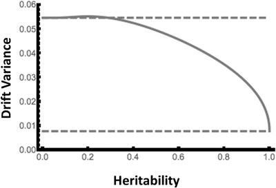
Genetic drift under truncation selection: The solid line gives the sampling variance in mean breeding value plotted against heritability of the trait under selection based on equation 4 in the main text with approximation for variance of genotypic fitness as given in Appendix 2. The upper dashed line gives the sampling variance under random sampling $(V_{A} (1 / N_{P} - 1 / 2 N))$ ⁠, and the lower dashed line gives the sampling variance under deterministic sampling $(V_{A} / 2 N)$ ⁠. The plot is based on a population size of N = 64 and a number of selected parents of N_p = 16, as in our experiment. The additive variance is set to V_A = 1 for illustration.

Open in new tab Download slide

To summarize, the expected variance of the prediction error after t generations is

\begin{matrix} V a r [{\bar{z}}_{t} - μ_{t}] = V a r [G_{z y}] β_{y}^{2} t^{2} \\ + V_{A} (\frac{1}{N_{P}} - \frac{1 + 3 F}{2 N (1 + F)} - \frac{V a r [w]}{N}) t + \frac{V_{e}}{N}, \end{matrix}

where G_zy is the additive covariance between the focal trait, z, and the trait under selection, y (which could be the focal trait itself). The variance in fitness is a function of the heritability of the trait under selection, which is not necessarily the focal trait. This prediction ignores the effects of selection and genetic drift on the G-matrix, which is assumed to stay constant throughout the experiment. Ideally, drift variance in the G-matrix should be added to the variance in the first term. The prediction also ignores the effects of sampling on the realized selection gradient, which will vary stochastically in a finite population, but this effect is not an error in the prediction from an observed selection gradient.

Materials and Methods

STUDY SPECIES AND TRAIT MEASUREMENTS

Dalechampia scandens (Euphorbiaceae) is a perennial Neotropical vine with flowers arranged in pseudanthial inflorescences (blossoms), each consisting of a male subinflorescence of 10 staminate flowers and a female subinflorescence of three pistillate flowers (Fig. 2). The male subinflorescence also contains a gland producing a triterpenoid resin as reward for pollinating bees that use resin in nest construction (Armbruster 1984, 1985, 1986, 1988, 1993), and the amount of resin offered to the pollinator depends on the gland size (Armbruster 1984; Pélabon et al. 2012). In interpopulation and interspecies comparisons, blossoms with larger resin glands tend to attract larger pollinators (Armbruster 1985, 1988). The blossom is subtended by two large involucral bracts, which are white or light green in the study species. Phenotypic selection studies on several Dalechampia species and populations have shown that pollinators choose blossoms based either on the size of the involucral bracts (the signal), or on the size of the gland (the reward), thus causing selection on these traits (Armbruster et al. 2005; Bolstad et al. 2010; Pérez-Barrales et al. 2013; Albertsen et al. 2021). Additionally, the Dalechampia blossom is an integrated structure in which involucral-bract size is phenotypically and genetically correlated with resin-gland size (Armbruster 1991; Hansen et al. 2003b; Armbruster et al. 2004; Pélabon et al. 2012). In this study, we performed artificial selection on the size of the resin-producing gland and recorded the direct response in gland size and the correlated response in bract size.

Figure 2

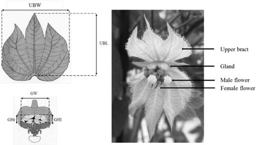
The Dalechampia blossom and the traits analyzed in this study. Gland area (GA) is the product of the average of the left and right gland height (GH_l and GH_r) and the total gland width (GW), and upper bract area (UBA) is the product of the upper bract width (UBW) and length (UBL) (Drawing by M. Carlson, Photo by E. Albertsen).

Open in new tab Download slide

Gland size was measured as the area of the resin-secreting surface (Gland Area, GA), and bract size was measured as the area of the upper bract (Upper Bract Area: UBA, see Fig. 2 for measurements details). Blossoms go through a series of ontogenetic stages during which they increase in size (Armbruster 1991; Opedal et al. 2016b). To reduce ontogenetic variation in size, we measured the blossoms on the first day of the bisexual phase, that is, when the first one-to-three male flowers were open. Measurements of the blossoms in the two diallels, the starting generation (F₀) and the first three episodes of selection were performed by one observer (CP) using 5× stereo magnifying lenses (Optivisor) and digital calipers with 0.01 mm precision. Measurements of the last generation were done by one observer (EA) using the same measuring devices. There was no evidence of systematic difference between observers in measurements on a common subset of blossoms, and because all selected lines were measured by a single observer at each generation, we do not expect the different observers to have affected the outcome of the study. During the diallels and the artificial-selection experiment, plants were placed randomly on four tables in a single room in the greenhouse of the Department of Biology, NTNU (Trondheim, Norway) and moved regularly during the measurement period to reduce positional effects.

Interpopulation crosses (Pélabon et al. 2004a, 2005) and molecular studies (Falahati-Anbaran et al. 2013, 2017) have shown that D. scandens is a complex of two or more distinct, yet undescribed species. In this study, diallels and artificial-selection experiments were performed on two populations from distinct species. Individuals from the first species are descended from seeds collected near Tulum, Mexico (20°13’ N; 87°26’ W), and individuals from the second species are descended from seeds collected near Tovar, Venezuela (8°21’ N; 71°46’ W).

DIALLEL EXPERIMENT

We estimated the G-matrix for several blossom traits in the two species with two diallels completed in 1999 to 2000 and in 2005 to 2006 for Tulum and Tovar, respectively. Methods and results of these diallels are presented in Bolstad et al. (2014). Briefly, seeds collected from different blossoms in the field were sown in the greenhouse and, upon maturity, plants were crossed in a partial diallel design with twelve and nine 5 × 5 blocks for Tulum and Tovar, respectively. Self and reciprocal crosses were included. Two seeds per cross were sown to produce the offspring generation (Tulum: n = 523 individuals; Tovar: n = 419 individuals) and two blossoms per individual were measured.

SELECTION EXPERIMENT

We conducted four episodes of selection on each species. Due to space limitation in the greenhouse, we alternated by generation the species being grown and measured, but the up- and down-selected lines as well as the control line from a given species were always grown simultaneously in the same room in the greenhouse with plants from the different lines placed randomly on the tables. To form the starting populations (F₀), we performed a stratified sampling of 100 individuals among the diallel blocks and families to have populations as similar as possible to the ones from which G-matrices were estimated. We did not include the diagonal of the diallel (i.e., selfed offspring) in this sampling. For Tovar, we sampled plants directly from the diallel experiment. For Tulum, whose diallel was completed first, all plants were selfed at the end of the diallel experiment and preserved as seeds until the start of the selection experiment. We sampled among these seeds to form the F₀ in Tulum, grew them, and measured their blossoms at maturation. Hence, the first episode of selection on the Tulum species was performed on selfed individuals.

This episode of selfing in the Tulum line may affect the response to selection by altering the trait mean due to dominance and by inflating additive variance by a factor of 1.5 for the first generation of selection (i.e., by 1+F, where F is the inbreeding coefficient, Lynch and Walsh 1998; Shaw et al. 1998). We thus multiplied G by 1.5 in our prediction for the first episode of selection in Tulum. We did not correct for dominance effects on the mean, however, because previous experiments with this species have shown little evidence of either dominance variance (Hansen et al. 2003a) or inbreeding effects (Pélabon et al. 2004b; Opedal et al. 2015).

We performed direct selection to increase or decrease the area of the resin-producing gland. We started the experiment by measuring gland and bract area on four blossoms per individual in the 100 individuals forming the F₀ and chose the 16 individuals with the smallest or largest mean gland area to produce the first generation of the down- and up-selected lines, respectively. Within each line, 64 new families were produced by pollinating each of the 16 individuals with pollen from four other individuals among the 16 selected. Each individual thus contributed equally to the next generation, four times as sire and four times as dam. Reciprocal crosses were avoided so that none of the 64 families shared more than one parent. Details of the crossing method and seed collection are presented in Pélabon et al. (2015). We kept track of the pedigree and never crossed individuals with a coefficient of relatedness higher than 0.10 to reduce inbreeding.

We sowed two or three seeds from each of the 64 families and kept one individual per family to form the F₁ generation. We then measured three blossoms per individual and selected the 16 (25%) most extreme individuals to produce the next generation. Selection gradients were calculated at each generation as the selection differential (mean of the selected individuals minus the mean of the population before selection) divided by the phenotypic variance of the line in that generation. From the F₁ generation and onwards, we maintained a population size of 64 individuals, and selected 16 of them. In practice, we kept the 20 most extreme individuals at each generation to replace individuals with poor blossom production to assure a total of 16 reproducing individuals. The number of individuals measured in each selected line at each generation varied slightly due to occasional failures to flower (Supporting Information S1 and S2).

For each species, we generated a control line from random crosses among individuals of the F₀ to assess phenotypic changes due to uncontrolled variation in the greenhouse environment. At each generation, several individuals from these control lines were grown simultaneously with the selected lines and randomly crossed while avoiding selfing to provide seeds for the next generation. For logistical reasons, the size of these control lines varied each generation (Appendix S1 and S2) and we were unable to measure them at the third generation (F₃).

The phenotypic values observed in the last generation (F₄) were unusual, particularly for bract size in the Tulum population (Appendix S3). This was most likely due to unusual conditions in the greenhouse. We thus regrew the last generation from seeds from the same crosses and measured it anew for both species. This second set of measurements provided qualitatively similar results as the first set regarding the differences between the up- and down-selected lines, but the phenotypic values were closer to the expected ones (see results). Therefore, we used this second set of measurements for the last generation in the analyses that follow.

STATISTICAL ANALYSES

Genetic parameters from the diallel experiment

The analyses of the two diallels are presented in Bolstad et al. (2014). For each species, we estimated the additive genetic variances and covariance for gland area and bract area together with their credible intervals. Using the R package MCMCglmm (Hadfield 2010) we fitted the following model:

z_{ijk} = μ_{i} + a_{ij} + b_{ij} + d_{ik} + s_{ijk} + q_{ijk},

where z is the trait value, μ the trait mean, a the breeding value, b the non-genetic plant effect, d, is the measurement date, s the number of male flowers open when the blossom was measured (1, 2, or 3), and q the within-plant residual effect. The subscripts i, j and k represent the trait, plant, and blossom, respectively. We accounted for temporal variation in the greenhouse environment by including measurement date d as a random factor. The random effects are assumed to be distributed as a∼N(0, G ⊗ A), b∼N(0, B ⊗ I), d∼N(0, F ⊗ I), and q∼N(0, E ⊗ I), where A is the relatedness matrix, I is the identity matrix and ⊗ is the Kronecker product. The model estimates the additive genetic variance matrix G, the among-plant environmental variance matrix B, the among-date variance matrix F, and the residual variance matrix E. The elements of the relatedness matrix are twice the coancestry coefficients of the corresponding relatives. The relevant coancestry coefficients are 1/2 for selfed full sibs, 1/4 for full sibs, and 1/8 for half-sibs. As priors for the Bayesian mixed models (MCMCglmm), we used zero-mean normal distributions with very large variances (10⁸) for the fixed effects, half-Cauchy distributions with scale parameter 20 for the variance components, and inverse-Wishart distributions for the residual variance matrices. These models ran for 1,100,000 iterations, with a burn-in phase of 100,000, and a thinning interval of 1000. Data were natural-log-transformed before analyses, so that evolutionary changes in the two traits could be interpreted as proportional changes and genetic variances as mean-scaled evolvabilities in the sense of Hansen et al. (2003a, 2011).

While the relatedness matrix accounts for known relatedness generated by the crosses in the diallel, it assumes that seeds collected in the wild are not inbred. This is problematic because D. scandens is self-compatible and can readily produce seeds by autogamy in absence of pollinators (Opedal et al. 2015, 2016a). Crosses among plants in the diallel experiment will remove this source of inbreeding, but within-plant crosses (diagonal of the diallel) may produce individuals with coefficients of coancestry larger than 0.5 and may upwardly bias the estimation of G. In absence of information about the level of inbreeding in each population, it is difficult to compute the element of the relatedness matrix. We therefore assessed the effect of parental inbreeding by analyzing the data from the two diallels with and without the selfed crosses. Except for a 40% reduction in the genetic variance of gland area in the Tulum population, the effects of removing selfed offspring were minor (Table S4 and Fig. S5). Because parental inbreeding would predict a proportional decrease of all elements in G, and because there was no effect in the Tovar population, which was a priori more likely to be inbred in view of its small herkogamy (Opedal et al. 2015, 2016a), it is unlikely that the observed differences are generated by inbreeding. We therefore used G estimated from the whole data set to calculate the predicted responses to selection and their intervals.

Comparing observed and predicted response to selection

We compared the observed responses to selection with the predictions from the multivariate Lande equation (Eq. 1) with genetic variances and covariances estimated from the two diallels. We constructed 95% prediction intervals from the variance in equation 7 by assuming that ${\bar{z}}_{t} - μ_{t}$ is normally distributed with mean zero. This is an approximation because the estimation errors of the elements in G are not normally distributed. We assumed no inbreeding (i.e., F = 0) in Tovar, and in Tulum, we multiplied G by 1.5 in the F₀ to account for the episode of selfing between the estimation of G and the start of the selection. Because crosses among selected parents avoided crosses among relatives, we further assumed no inbreeding from the F₁ and onward.

To control for variation in the greenhouse environment across generations, we centered the response to selection on the mean of the up- and down-selected lines or we corrected the responses for changes in the control line. In the former case, the responses of the up- and down-selected lines are forced to be symmetrical. This approach also assumes that environmental effects are identical in the up- and down-selected lines. Correcting for changes in the control line avoids these assumptions but yields less precise predictions due to the estimation error in the control mean.

Analyzing the temporal dynamics of the responses to selection

In a second set of analyses, we used the R package SRA (Selection Response Analysis; Le Rouzic et al. 2011) to estimate the realized genetic parameters from the observed response to selection. The SRA package fits deterministic population-genetics models with different genetic architectures (e.g., epistasis, linkage disequilibrium, or finite number of loci) to time series of selection responses (Le Rouzic et al. 2010, 2011, Le Rouzic 2014). These analyses therefore assess the influence of discrepancies between the model chosen to make the predictions (Lande equation) and the evolutionary processes that generated the selection responses. The code was modified to include two traits, one selected and one correlated, and to estimate the genetic covariance between them (Supporting Information S6). The model estimates the realized additive genetic variance of the selected trait, V_A, and covariance, G_zy, with the correlated trait, as well as the environmental variances E_z and E_y. It is not possible to estimate the realized additive genetic variance for the correlated trait because direct selection on this trait is assumed to be zero. The full dataset needed to fit the time-series model included for each generation, the sample size, the phenotypic means for both traits before and after selection, and their associated phenotypic variances (Supporting Information S1 and S2).

Although often assumed to be constant over a few episodes of selection, G may change due to allele-frequency changes, directional epistasis, and changes in linkage disequilibrium (the Bulmer effect; Bulmer 1971). We compared models fitted with or without a Bulmer effect, but due to the limited number of generations, we could not fit more complex models including epistasis or major-effect loci. We also tested for the occurrence of asymmetry in the response to selection (e.g., Bohren et al. 1966; Frankham 1990; Bell 2008, Walsh and Lynch 2018 chapter 18) by allowing variances to differ in the two selected directions with and without correcting for changes in the control line.

At each generation, we calculated the phenotypic correlation and the slope of the regression of log(UBA) on log(GA) using mixed-effect models with plant identity as a random effect. All statistical analyses were performed with R 4.0.2 (R core team, 2020).

Results

GENETIC VARIATION AND EVOLVABILITY

The G-matrices estimated from the two diallels are presented in Table 1. Because we conducted analyses on natural-log-transformed data, the additive genetic variances can be interpreted as mean-scaled evolvabilities sensu Hansen et al. (2003a, 2011). The unconditional evolvabilities of gland and bract area were 1.05% and 1.41% in Tovar and 0.73% and 0.84% in Tulum. These are moderately high evolvabilities for morphological traits (Hansen and Pélabon 2021). The genetic covariances between the two traits were 0.57 in Tovar and 0.49 in Tulum, which should generate robust correlated responses to selection. The correlations are not strong enough to constitute a major constraint on evolution, however, because conditioning traits on each other, sensu Hansen et al. (2003b), would only reduce their evolvabilities by 22% in Tovar and 40% in Tulum.

Table 1

Open in new tab

Trait means (SD), genetic (G), environmental (E), and phenotypic (P) variance matrices for the Tovar and Tulum populations of Dalechampia scandens estimated from the diallel experiments with the full data set (including selfed)

			Gland area (GA)	Upper bract area (UBA)
Tovar	mean (SD)		17.56 (3.30) mm²	385.0 (75.7) mm²
	G	GA	1.05 ±0.20 (0.69; 1.44)	0.57 ±0.15 (0.30; 0.87)
		UBA	0.47 ±0.08 (0.30; 0.62)	1.41 ±0.20 (1.07; 1.80)
	E	GA	2.27 ±0.16 (1.93; 2.55)	1.14 ±0.11 (0.95; 1.35)
		UBA	0.57 ±0.03 (0.51; 0.63)	1.76 ±0.12 (1.56; 2.02)
	P	GA	3.32 ±0.19 (2.98; 3.68)	1.72 ±0.15 (1.44; 1.99)
		UBA	0.53 ±0.03 (0.47; 0.58)	3.17 ±0.19 (2.84; 3.60)
Tulum	mean (SD)		20.20 (5.26) mm²	407.0 (81.9) mm²
	G	GA	0.73 ±0.22 (0.37; 1.16)	0.49 ±0.13 (0.23; 0.75)
		UBA	0.63 ±0.11 (0.43; 0.82)	0.84 ±0.14 (0.60; 1.13)
	E	GA	5.63 ±0.30 (5.03; 6.20)	1.60 ±0.15 (1.29; 1.87)
		UBA	0.45 ±0.03 (0.38; 0.50)	2.27 ±0.13 (2.06; 2.53)
	P	GA	6.36 ±0.28 (5.82; 6.91)	2.09 ±0.16 (1.78; 2.37)
		UBA	0.47 ±0.03 (0.41; 0.51)	3.11 ±0.15 (2.81; 3.41)

			Gland area (GA)	Upper bract area (UBA)
Tovar	mean (SD)		17.56 (3.30) mm²	385.0 (75.7) mm²
	G	GA	1.05 ±0.20 (0.69; 1.44)	0.57 ±0.15 (0.30; 0.87)
		UBA	0.47 ±0.08 (0.30; 0.62)	1.41 ±0.20 (1.07; 1.80)
	E	GA	2.27 ±0.16 (1.93; 2.55)	1.14 ±0.11 (0.95; 1.35)
		UBA	0.57 ±0.03 (0.51; 0.63)	1.76 ±0.12 (1.56; 2.02)
	P	GA	3.32 ±0.19 (2.98; 3.68)	1.72 ±0.15 (1.44; 1.99)
		UBA	0.53 ±0.03 (0.47; 0.58)	3.17 ±0.19 (2.84; 3.60)
Tulum	mean (SD)		20.20 (5.26) mm²	407.0 (81.9) mm²
	G	GA	0.73 ±0.22 (0.37; 1.16)	0.49 ±0.13 (0.23; 0.75)
		UBA	0.63 ±0.11 (0.43; 0.82)	0.84 ±0.14 (0.60; 1.13)
	E	GA	5.63 ±0.30 (5.03; 6.20)	1.60 ±0.15 (1.29; 1.87)
		UBA	0.45 ±0.03 (0.38; 0.50)	2.27 ±0.13 (2.06; 2.53)
	P	GA	6.36 ±0.28 (5.82; 6.91)	2.09 ±0.16 (1.78; 2.37)
		UBA	0.47 ±0.03 (0.41; 0.51)	3.11 ±0.15 (2.81; 3.41)

For each matrix, variances are reported on the diagonal, covariances above, and correlations below the diagonal along with their standard error and credible intervals (genetic; calculated with HPDinterval.mcmc with default probability = 0.95) or confidence intervals (phenotypic) between parentheses. Means and SDs are in mm², variances and covariances are in log(mm²) × 100. The E variance matrices are sums of two components: the residual of the diallel model and the individual error level. Genetic correlations are estimated from the posterior distribution of the MCMCglmm models estimating genetic variances and covariances between GA and UBA. Sample size are 820 for Tovar and 1046 for Tulum.

Table 1

Open in new tab

			Gland area (GA)	Upper bract area (UBA)
Tovar	mean (SD)		17.56 (3.30) mm²	385.0 (75.7) mm²
	G	GA	1.05 ±0.20 (0.69; 1.44)	0.57 ±0.15 (0.30; 0.87)
		UBA	0.47 ±0.08 (0.30; 0.62)	1.41 ±0.20 (1.07; 1.80)
	E	GA	2.27 ±0.16 (1.93; 2.55)	1.14 ±0.11 (0.95; 1.35)
		UBA	0.57 ±0.03 (0.51; 0.63)	1.76 ±0.12 (1.56; 2.02)
	P	GA	3.32 ±0.19 (2.98; 3.68)	1.72 ±0.15 (1.44; 1.99)
		UBA	0.53 ±0.03 (0.47; 0.58)	3.17 ±0.19 (2.84; 3.60)
Tulum	mean (SD)		20.20 (5.26) mm²	407.0 (81.9) mm²
	G	GA	0.73 ±0.22 (0.37; 1.16)	0.49 ±0.13 (0.23; 0.75)
		UBA	0.63 ±0.11 (0.43; 0.82)	0.84 ±0.14 (0.60; 1.13)
	E	GA	5.63 ±0.30 (5.03; 6.20)	1.60 ±0.15 (1.29; 1.87)
		UBA	0.45 ±0.03 (0.38; 0.50)	2.27 ±0.13 (2.06; 2.53)
	P	GA	6.36 ±0.28 (5.82; 6.91)	2.09 ±0.16 (1.78; 2.37)
		UBA	0.47 ±0.03 (0.41; 0.51)	3.11 ±0.15 (2.81; 3.41)

			Gland area (GA)	Upper bract area (UBA)
Tovar	mean (SD)		17.56 (3.30) mm²	385.0 (75.7) mm²
	G	GA	1.05 ±0.20 (0.69; 1.44)	0.57 ±0.15 (0.30; 0.87)
		UBA	0.47 ±0.08 (0.30; 0.62)	1.41 ±0.20 (1.07; 1.80)
	E	GA	2.27 ±0.16 (1.93; 2.55)	1.14 ±0.11 (0.95; 1.35)
		UBA	0.57 ±0.03 (0.51; 0.63)	1.76 ±0.12 (1.56; 2.02)
	P	GA	3.32 ±0.19 (2.98; 3.68)	1.72 ±0.15 (1.44; 1.99)
		UBA	0.53 ±0.03 (0.47; 0.58)	3.17 ±0.19 (2.84; 3.60)
Tulum	mean (SD)		20.20 (5.26) mm²	407.0 (81.9) mm²
	G	GA	0.73 ±0.22 (0.37; 1.16)	0.49 ±0.13 (0.23; 0.75)
		UBA	0.63 ±0.11 (0.43; 0.82)	0.84 ±0.14 (0.60; 1.13)
	E	GA	5.63 ±0.30 (5.03; 6.20)	1.60 ±0.15 (1.29; 1.87)
		UBA	0.45 ±0.03 (0.38; 0.50)	2.27 ±0.13 (2.06; 2.53)
	P	GA	6.36 ±0.28 (5.82; 6.91)	2.09 ±0.16 (1.78; 2.37)
		UBA	0.47 ±0.03 (0.41; 0.51)	3.11 ±0.15 (2.81; 3.41)

DIRECT RESPONSE TO SELECTION

Gland area responded to selection in both species, but the response diminished after the second generation (Fig. 3 and 4; Supporting Information S3), and despite a good fit in the first generation, responses after four episodes of selection were nearly half the prediction for the Tovar lines and 30% lower for the Tulum lines. Still, observed responses remained within the 95% prediction intervals, although barely so for Tovar. Thus, if we neglect the temporal dynamics of the response, the discrepancies could be explained by a combination of sampling stochasticity in the response and uncertainty in the prediction due to estimation error in the additive genetic variance (Table 2). For the mean-centered responses (Fig. 3), 60% to 70% of the prediction error variance was due to sampling effects in the first generation, but by the last generation this has shifted to almost 80% being due to estimation error in the additive variance. For the control-corrected responses (Fig. 4), the contribution of the sampling effects was larger and remained above 50% of the total error variance even after four episodes of selection (Table 2).

Figure 3

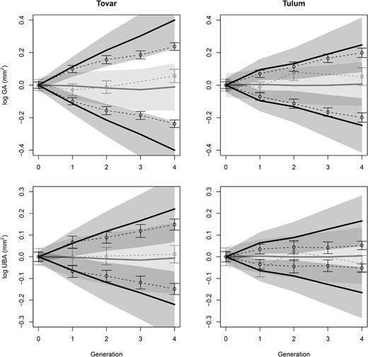
Observed and predicted response to selection with data centered on the generation mean of the up- and down-selected lines. For the two species of D. scandens the responses are shown for gland area (GA), which is the selected trait, and bract area (UBA), which is the correlated trait. Observed responses in trait means (±2SE) are given as the dotted lines. The predicted responses with their prediction intervals (±2SE) are represented by the black lines and shaded area. Control lines are reported in grey with their prediction intervals in light grey.

Open in new tab Download slide

Figure 4

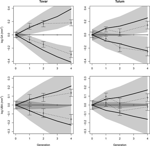
Observed and predicted response to selection with responses corrected for changes in the control lines. No results are given for the 3^rd generation due to the absence of a control. See Figure 3 for definitions of symbols and shaded areas.

Open in new tab Download slide

Table 2

Open in new tab

Contribution of the different sources of uncertainty to the prediction intervals for data centered on the mean of the Up- and Down-selected lines (Up-Down centered) or corrected for changes in the control line (Control corrected)

			Source of error			Up-down centered							Control corrected
	Trait	Gen.	G	D	E	Var^#	%G	%D	%E	Resp.	2SE	Rel. err.	Var^$	%G	%D	%E	2SE	Rel. err.
Tovar	GA	0	0.0	0.0	3.6	1.8	0.0	0.0	100.0	0.00	0.03	NA	7.1	0.0	0.0	100.0	0.05	NA
		1	3.8	7.8	3.6	9.4	40.0	41.1	18.9	0.11	0.06	27.2	26.4	14.3	58.7	27.0	0.10	45.6
		2	15.1	15.5	3.6	24.7	61.3	31.5	7.2	0.21	0.10	23.1	53.3	28.3	58.3	13.4	0.15	34.0
		3	34.0	23.3	3.6	47.4	71.7	24.6	3.8	0.30	0.14	22.7	87.7	38.8	53.1	8.1	0.19	30.9
		4	60.4	31.1	3.6	77.8	77.7	20.0	2.3	0.40	0.18	22.0	129.7	46.6	47.9	5.5	0.23	28.5
	UBA	0	0.0	0.0	2.8	1.4	0.0	0.0	100.0	0.00	0.02	NA	5.5	0.0	0.0	100.0	0.05	NA
		1	2.2	10.6	2.8	8.9	24.8	59.7	15.5	0.06	0.06	48.0	28.9	7.6	73.3	19.1	0.11	86.6
		2	8.8	21.2	2.8	20.8	42.4	51.0	6.6	0.12	0.09	38.5	56.7	15.5	74.8	9.7	0.15	63.7
		3	19.8	31.8	2.8	37.0	53.4	42.9	3.7	0.17	0.12	36.5	88.8	22.3	71.5	6.2	0.19	56.6
		4	35.2	42.4	2.8	57.7	60.9	36.7	2.4	0.22	0.15	34.5	125.4	28.1	67.6	4.4	0.22	50.9
Tulum	GA	0	0.0	0.0	8.8	4.4	0.0	0.0	100.0	0.00	0.04	NA	17.6	0.0	0.0	100.0	0.08	NA
		1	3.4	5.4	8.8	10.6	32.5	25.7	41.7	0.10	0.06	34.0	31.9	10.8	34.0	55.2	0.11	59.2
		2	13.7	10.9	8.8	23.6	58.3	23.0	18.7	0.13	0.10	36.7	53.1	25.9	40.9	33.2	0.15	55.0
		3	30.9	16.3	8.8	43.4	71.1	18.8	10.1	0.19	0.13	34.5	81.1	38.1	40.2	21.7	0.18	47.2
		4	54.9	21.7	8.8	70.2	78.2	15.5	6.3	0.25	0.17	33.8	116.0	47.4	37.5	15.2	0.22	43.5
	UBA	0	0.0	0.0	3.6	1.8	0.0	0.0	100.0	0.00	0.03	NA	7.1	0.0	0.0	100.0	0.05	NA
		1	1.3	6.2	3.6	6.2	20.6	50.5	28.9	0.06	0.05	39.0	20.9	6.1	59.7	34.2	0.09	71.6
		2	5.1	12.5	3.6	13.1	38.8	47.5	13.6	0.09	0.07	40.9	37.1	13.7	67.1	19.2	0.12	68.9
		3	11.4	18.7	3.6	22.6	50.7	41.4	7.9	0.13	0.10	37.3	55.9	20.5	66.8	12.8	0.15	58.6
		4	20.3	24.9	3.6	34.6	58.8	36.0	5.2	0.17	0.12	35.6	77.3	26.3	64.5	9.2	0.18	53.2

			Source of error			Up-down centered							Control corrected
	Trait	Gen.	G	D	E	Var^#	%G	%D	%E	Resp.	2SE	Rel. err.	Var^$	%G	%D	%E	2SE	Rel. err.
Tovar	GA	0	0.0	0.0	3.6	1.8	0.0	0.0	100.0	0.00	0.03	NA	7.1	0.0	0.0	100.0	0.05	NA
		1	3.8	7.8	3.6	9.4	40.0	41.1	18.9	0.11	0.06	27.2	26.4	14.3	58.7	27.0	0.10	45.6
		2	15.1	15.5	3.6	24.7	61.3	31.5	7.2	0.21	0.10	23.1	53.3	28.3	58.3	13.4	0.15	34.0
		3	34.0	23.3	3.6	47.4	71.7	24.6	3.8	0.30	0.14	22.7	87.7	38.8	53.1	8.1	0.19	30.9
		4	60.4	31.1	3.6	77.8	77.7	20.0	2.3	0.40	0.18	22.0	129.7	46.6	47.9	5.5	0.23	28.5
	UBA	0	0.0	0.0	2.8	1.4	0.0	0.0	100.0	0.00	0.02	NA	5.5	0.0	0.0	100.0	0.05	NA
		1	2.2	10.6	2.8	8.9	24.8	59.7	15.5	0.06	0.06	48.0	28.9	7.6	73.3	19.1	0.11	86.6
		2	8.8	21.2	2.8	20.8	42.4	51.0	6.6	0.12	0.09	38.5	56.7	15.5	74.8	9.7	0.15	63.7
		3	19.8	31.8	2.8	37.0	53.4	42.9	3.7	0.17	0.12	36.5	88.8	22.3	71.5	6.2	0.19	56.6
		4	35.2	42.4	2.8	57.7	60.9	36.7	2.4	0.22	0.15	34.5	125.4	28.1	67.6	4.4	0.22	50.9
Tulum	GA	0	0.0	0.0	8.8	4.4	0.0	0.0	100.0	0.00	0.04	NA	17.6	0.0	0.0	100.0	0.08	NA
		1	3.4	5.4	8.8	10.6	32.5	25.7	41.7	0.10	0.06	34.0	31.9	10.8	34.0	55.2	0.11	59.2
		2	13.7	10.9	8.8	23.6	58.3	23.0	18.7	0.13	0.10	36.7	53.1	25.9	40.9	33.2	0.15	55.0
		3	30.9	16.3	8.8	43.4	71.1	18.8	10.1	0.19	0.13	34.5	81.1	38.1	40.2	21.7	0.18	47.2
		4	54.9	21.7	8.8	70.2	78.2	15.5	6.3	0.25	0.17	33.8	116.0	47.4	37.5	15.2	0.22	43.5
	UBA	0	0.0	0.0	3.6	1.8	0.0	0.0	100.0	0.00	0.03	NA	7.1	0.0	0.0	100.0	0.05	NA
		1	1.3	6.2	3.6	6.2	20.6	50.5	28.9	0.06	0.05	39.0	20.9	6.1	59.7	34.2	0.09	71.6
		2	5.1	12.5	3.6	13.1	38.8	47.5	13.6	0.09	0.07	40.9	37.1	13.7	67.1	19.2	0.12	68.9
		3	11.4	18.7	3.6	22.6	50.7	41.4	7.9	0.13	0.10	37.3	55.9	20.5	66.8	12.8	0.15	58.6
		4	20.3	24.9	3.6	34.6	58.8	36.0	5.2	0.17	0.12	35.6	77.3	26.3	64.5	9.2	0.18	53.2

# Var = V_A + ½ × Drift + ½ × Env.

$ Var = V_A + 2 × Drift + 2 × Env.

Uncertainties in 100 × (log(mm²))² are due to error in genetic parameters, G, genetic drift, D, and environmental variation, E (see Eq. 7 for the calculation of each contribution). The total error variance is reported in the Var columns and the relative contributions are reported in the columns %G, %D and %E, respectively. The width of the prediction intervals in Fig. 3 and 4 are calculated as $2 S E = 2 \sqrt{V a r} / 100$ ⁠. We also give the relative error (Rel.) in the predicted response (Resp.) as 100 × SE/Resp.

Table 2

Open in new tab

			Source of error			Up-down centered							Control corrected
	Trait	Gen.	G	D	E	Var^#	%G	%D	%E	Resp.	2SE	Rel. err.	Var^$	%G	%D	%E	2SE	Rel. err.
Tovar	GA	0	0.0	0.0	3.6	1.8	0.0	0.0	100.0	0.00	0.03	NA	7.1	0.0	0.0	100.0	0.05	NA
		1	3.8	7.8	3.6	9.4	40.0	41.1	18.9	0.11	0.06	27.2	26.4	14.3	58.7	27.0	0.10	45.6
		2	15.1	15.5	3.6	24.7	61.3	31.5	7.2	0.21	0.10	23.1	53.3	28.3	58.3	13.4	0.15	34.0
		3	34.0	23.3	3.6	47.4	71.7	24.6	3.8	0.30	0.14	22.7	87.7	38.8	53.1	8.1	0.19	30.9
		4	60.4	31.1	3.6	77.8	77.7	20.0	2.3	0.40	0.18	22.0	129.7	46.6	47.9	5.5	0.23	28.5
	UBA	0	0.0	0.0	2.8	1.4	0.0	0.0	100.0	0.00	0.02	NA	5.5	0.0	0.0	100.0	0.05	NA
		1	2.2	10.6	2.8	8.9	24.8	59.7	15.5	0.06	0.06	48.0	28.9	7.6	73.3	19.1	0.11	86.6
		2	8.8	21.2	2.8	20.8	42.4	51.0	6.6	0.12	0.09	38.5	56.7	15.5	74.8	9.7	0.15	63.7
		3	19.8	31.8	2.8	37.0	53.4	42.9	3.7	0.17	0.12	36.5	88.8	22.3	71.5	6.2	0.19	56.6
		4	35.2	42.4	2.8	57.7	60.9	36.7	2.4	0.22	0.15	34.5	125.4	28.1	67.6	4.4	0.22	50.9
Tulum	GA	0	0.0	0.0	8.8	4.4	0.0	0.0	100.0	0.00	0.04	NA	17.6	0.0	0.0	100.0	0.08	NA
		1	3.4	5.4	8.8	10.6	32.5	25.7	41.7	0.10	0.06	34.0	31.9	10.8	34.0	55.2	0.11	59.2
		2	13.7	10.9	8.8	23.6	58.3	23.0	18.7	0.13	0.10	36.7	53.1	25.9	40.9	33.2	0.15	55.0
		3	30.9	16.3	8.8	43.4	71.1	18.8	10.1	0.19	0.13	34.5	81.1	38.1	40.2	21.7	0.18	47.2
		4	54.9	21.7	8.8	70.2	78.2	15.5	6.3	0.25	0.17	33.8	116.0	47.4	37.5	15.2	0.22	43.5
	UBA	0	0.0	0.0	3.6	1.8	0.0	0.0	100.0	0.00	0.03	NA	7.1	0.0	0.0	100.0	0.05	NA
		1	1.3	6.2	3.6	6.2	20.6	50.5	28.9	0.06	0.05	39.0	20.9	6.1	59.7	34.2	0.09	71.6
		2	5.1	12.5	3.6	13.1	38.8	47.5	13.6	0.09	0.07	40.9	37.1	13.7	67.1	19.2	0.12	68.9
		3	11.4	18.7	3.6	22.6	50.7	41.4	7.9	0.13	0.10	37.3	55.9	20.5	66.8	12.8	0.15	58.6
		4	20.3	24.9	3.6	34.6	58.8	36.0	5.2	0.17	0.12	35.6	77.3	26.3	64.5	9.2	0.18	53.2

			Source of error			Up-down centered							Control corrected
	Trait	Gen.	G	D	E	Var^#	%G	%D	%E	Resp.	2SE	Rel. err.	Var^$	%G	%D	%E	2SE	Rel. err.
Tovar	GA	0	0.0	0.0	3.6	1.8	0.0	0.0	100.0	0.00	0.03	NA	7.1	0.0	0.0	100.0	0.05	NA
		1	3.8	7.8	3.6	9.4	40.0	41.1	18.9	0.11	0.06	27.2	26.4	14.3	58.7	27.0	0.10	45.6
		2	15.1	15.5	3.6	24.7	61.3	31.5	7.2	0.21	0.10	23.1	53.3	28.3	58.3	13.4	0.15	34.0
		3	34.0	23.3	3.6	47.4	71.7	24.6	3.8	0.30	0.14	22.7	87.7	38.8	53.1	8.1	0.19	30.9
		4	60.4	31.1	3.6	77.8	77.7	20.0	2.3	0.40	0.18	22.0	129.7	46.6	47.9	5.5	0.23	28.5
	UBA	0	0.0	0.0	2.8	1.4	0.0	0.0	100.0	0.00	0.02	NA	5.5	0.0	0.0	100.0	0.05	NA
		1	2.2	10.6	2.8	8.9	24.8	59.7	15.5	0.06	0.06	48.0	28.9	7.6	73.3	19.1	0.11	86.6
		2	8.8	21.2	2.8	20.8	42.4	51.0	6.6	0.12	0.09	38.5	56.7	15.5	74.8	9.7	0.15	63.7
		3	19.8	31.8	2.8	37.0	53.4	42.9	3.7	0.17	0.12	36.5	88.8	22.3	71.5	6.2	0.19	56.6
		4	35.2	42.4	2.8	57.7	60.9	36.7	2.4	0.22	0.15	34.5	125.4	28.1	67.6	4.4	0.22	50.9
Tulum	GA	0	0.0	0.0	8.8	4.4	0.0	0.0	100.0	0.00	0.04	NA	17.6	0.0	0.0	100.0	0.08	NA
		1	3.4	5.4	8.8	10.6	32.5	25.7	41.7	0.10	0.06	34.0	31.9	10.8	34.0	55.2	0.11	59.2
		2	13.7	10.9	8.8	23.6	58.3	23.0	18.7	0.13	0.10	36.7	53.1	25.9	40.9	33.2	0.15	55.0
		3	30.9	16.3	8.8	43.4	71.1	18.8	10.1	0.19	0.13	34.5	81.1	38.1	40.2	21.7	0.18	47.2
		4	54.9	21.7	8.8	70.2	78.2	15.5	6.3	0.25	0.17	33.8	116.0	47.4	37.5	15.2	0.22	43.5
	UBA	0	0.0	0.0	3.6	1.8	0.0	0.0	100.0	0.00	0.03	NA	7.1	0.0	0.0	100.0	0.05	NA
		1	1.3	6.2	3.6	6.2	20.6	50.5	28.9	0.06	0.05	39.0	20.9	6.1	59.7	34.2	0.09	71.6
		2	5.1	12.5	3.6	13.1	38.8	47.5	13.6	0.09	0.07	40.9	37.1	13.7	67.1	19.2	0.12	68.9
		3	11.4	18.7	3.6	22.6	50.7	41.4	7.9	0.13	0.10	37.3	55.9	20.5	66.8	12.8	0.15	58.6
		4	20.3	24.9	3.6	34.6	58.8	36.0	5.2	0.17	0.12	35.6	77.3	26.3	64.5	9.2	0.18	53.2

# Var = V_A + ½ × Drift + ½ × Env.

$ Var = V_A + 2 × Drift + 2 × Env.

The realized evolvabilities estimated from the selection response analysis were smaller than the evolvabilities estimated from the diallels (Table 3). Including a Bulmer effect improved the fit for the Tovar data, but had little impact on the estimated evolvabilities. When corrected for changes in the control lines, the direct responses in gland area were asymmetrical, with a larger decrease for both species (Table 3).

Table 3

Open in new tab

Estimated (diallel) and realized (artificial selection) genetic variance of gland area (GA) and covariance between gland area and upper bract area (UBA) in the two species of D. scandens

Species	Data	Method	ΔAICc	Direction	G_log(GA)	G_{log(GA), log(UBA)}
Tovar	Diallel	MCMCglmm			1.05 (0.69; 1.44)	0.57 (0.30; 0.87)
	Up-Down centered	Symmetric	359.9		0.49 (0.46; 0.52)	0.33 (0.30; 0.37)
		Symmetric + Bulmer^§	352.5		0.53 (0.50; 0.57)	0.33 (0.30; 0.37)
	Raw data	Asymmetric	1.4	Up	0.26 (0.21; 0.32)	0.52 (0.46; 0.59)
				Down	0.72 (0.66; 0.78)	0.17 (0.11; 0.24)
		Asymmetric + Bulmer	0	Up	0.27 (0.21; 0.34)	0.52 (0.45; 0.59)
				Down	0.80 (0.73; 0.87)	0.17 (0.11; 0.24)
	Control-corrected	Symmetric	239.8		0.49 (0.46; 0.52)	0.34 (0.31; 0.37)
		Symmetric + Bulmer^§	234.6		0.54 (0.50; 0.58)	0.34 (0.31; 0.37)
		Asymmetric	1.6	Up	0.40 (0.34; 0.46)	0.33 (0.27; 0.40)
				Down	0.58 (0.53; 0.65)	0.35 (0.29; 0.41)
		Asymmetric + Bulmer	0	Up	0.44 (0.38; 0.51)	0.34 (0.27; 0.40)
				Down	0.63 (0.57; 0.70)	0.35 (0.29; 0.41)
Tulum	Diallel	MCMCglmm			0.73 (0.37; 1.16)	0.49 (0.23; 0.75)
	Up-Down centered	Symmetric	462.8		0.38 (0.34; 0.42)	0.14 (0.11; 0.17)
		Symmetric + Bulmer^§	462.8		0.39 (0.35; 0.43)	0.14 (0.11; 0.17)
	Raw data	Asymmetric	0	Up	0 (0; Inf)	0.17 (0.11; 0.19)
				Down	0.84 (0.78; 0.9)	0.13 (0.07; 0.19)
		Asymmetric + Bulmer	5.5	Up	0 (0; Inf)	0.17 (0.11; 0.23)
				Down	0.90 (0.83; 0.97)	0.13 (0.07; 0.19)
	Control-corrected	Symmetric	242.0		0.38 (0.35; 0.42)	0.15 (0.11; 0.18)
		Symmetric + Bulmer^§	243.0		0.40 (0.36; 0.44)	0.15 (0.11; 0.18)
		Asymmetric	0	Up	0.27 (0.22; 0.34)	0.16 (0.10; 0.22)
				Down	0.51 (0.45; 0.58)	0.13 (0.07; 0.20)
		Asymmetric + Bulmer	1.6	Up	0.28 (0.22; 0.35)	0.16 (0.10; 0.22)
				Down	0.53 (0.46; 0.61)	0.13 (0.07; 0.20)

Species	Data	Method	ΔAICc	Direction	G_log(GA)	G_{log(GA), log(UBA)}
Tovar	Diallel	MCMCglmm			1.05 (0.69; 1.44)	0.57 (0.30; 0.87)
	Up-Down centered	Symmetric	359.9		0.49 (0.46; 0.52)	0.33 (0.30; 0.37)
		Symmetric + Bulmer^§	352.5		0.53 (0.50; 0.57)	0.33 (0.30; 0.37)
	Raw data	Asymmetric	1.4	Up	0.26 (0.21; 0.32)	0.52 (0.46; 0.59)
				Down	0.72 (0.66; 0.78)	0.17 (0.11; 0.24)
		Asymmetric + Bulmer	0	Up	0.27 (0.21; 0.34)	0.52 (0.45; 0.59)
				Down	0.80 (0.73; 0.87)	0.17 (0.11; 0.24)
	Control-corrected	Symmetric	239.8		0.49 (0.46; 0.52)	0.34 (0.31; 0.37)
		Symmetric + Bulmer^§	234.6		0.54 (0.50; 0.58)	0.34 (0.31; 0.37)
		Asymmetric	1.6	Up	0.40 (0.34; 0.46)	0.33 (0.27; 0.40)
				Down	0.58 (0.53; 0.65)	0.35 (0.29; 0.41)
		Asymmetric + Bulmer	0	Up	0.44 (0.38; 0.51)	0.34 (0.27; 0.40)
				Down	0.63 (0.57; 0.70)	0.35 (0.29; 0.41)
Tulum	Diallel	MCMCglmm			0.73 (0.37; 1.16)	0.49 (0.23; 0.75)
	Up-Down centered	Symmetric	462.8		0.38 (0.34; 0.42)	0.14 (0.11; 0.17)
		Symmetric + Bulmer^§	462.8		0.39 (0.35; 0.43)	0.14 (0.11; 0.17)
	Raw data	Asymmetric	0	Up	0 (0; Inf)	0.17 (0.11; 0.19)
				Down	0.84 (0.78; 0.9)	0.13 (0.07; 0.19)
		Asymmetric + Bulmer	5.5	Up	0 (0; Inf)	0.17 (0.11; 0.23)
				Down	0.90 (0.83; 0.97)	0.13 (0.07; 0.19)
	Control-corrected	Symmetric	242.0		0.38 (0.35; 0.42)	0.15 (0.11; 0.18)
		Symmetric + Bulmer^§	243.0		0.40 (0.36; 0.44)	0.15 (0.11; 0.18)
		Asymmetric	0	Up	0.27 (0.22; 0.34)	0.16 (0.10; 0.22)
				Down	0.51 (0.45; 0.58)	0.13 (0.07; 0.20)
		Asymmetric + Bulmer	1.6	Up	0.28 (0.22; 0.35)	0.16 (0.10; 0.22)
				Down	0.53 (0.46; 0.61)	0.13 (0.07; 0.20)

The bivariate SRA models assume constant genetic covariance (see Appendix S6), therefore estimates of the genetic covariance are not affected by the Bulmer effect.

All estimates are calculated from log-transformed data and × 100. Estimates for the realized responses are calculated for the pooled up- and down-selected lines assuming symmetric response, with or without Bulmer effect, or assuming different variances in the up and down lines, using the raw data or the data corrected for the control (95% credible intervals for the estimated parameters and 95% confidence interval for the realized values in parentheses).

Table 3

Open in new tab

Estimated (diallel) and realized (artificial selection) genetic variance of gland area (GA) and covariance between gland area and upper bract area (UBA) in the two species of D. scandens

Species	Data	Method	ΔAICc	Direction	G_log(GA)	G_{log(GA), log(UBA)}
Tovar	Diallel	MCMCglmm			1.05 (0.69; 1.44)	0.57 (0.30; 0.87)
	Up-Down centered	Symmetric	359.9		0.49 (0.46; 0.52)	0.33 (0.30; 0.37)
		Symmetric + Bulmer^§	352.5		0.53 (0.50; 0.57)	0.33 (0.30; 0.37)
	Raw data	Asymmetric	1.4	Up	0.26 (0.21; 0.32)	0.52 (0.46; 0.59)
				Down	0.72 (0.66; 0.78)	0.17 (0.11; 0.24)
		Asymmetric + Bulmer	0	Up	0.27 (0.21; 0.34)	0.52 (0.45; 0.59)
				Down	0.80 (0.73; 0.87)	0.17 (0.11; 0.24)
	Control-corrected	Symmetric	239.8		0.49 (0.46; 0.52)	0.34 (0.31; 0.37)
		Symmetric + Bulmer^§	234.6		0.54 (0.50; 0.58)	0.34 (0.31; 0.37)
		Asymmetric	1.6	Up	0.40 (0.34; 0.46)	0.33 (0.27; 0.40)
				Down	0.58 (0.53; 0.65)	0.35 (0.29; 0.41)
		Asymmetric + Bulmer	0	Up	0.44 (0.38; 0.51)	0.34 (0.27; 0.40)
				Down	0.63 (0.57; 0.70)	0.35 (0.29; 0.41)
Tulum	Diallel	MCMCglmm			0.73 (0.37; 1.16)	0.49 (0.23; 0.75)
	Up-Down centered	Symmetric	462.8		0.38 (0.34; 0.42)	0.14 (0.11; 0.17)
		Symmetric + Bulmer^§	462.8		0.39 (0.35; 0.43)	0.14 (0.11; 0.17)
	Raw data	Asymmetric	0	Up	0 (0; Inf)	0.17 (0.11; 0.19)
				Down	0.84 (0.78; 0.9)	0.13 (0.07; 0.19)
		Asymmetric + Bulmer	5.5	Up	0 (0; Inf)	0.17 (0.11; 0.23)
				Down	0.90 (0.83; 0.97)	0.13 (0.07; 0.19)
	Control-corrected	Symmetric	242.0		0.38 (0.35; 0.42)	0.15 (0.11; 0.18)
		Symmetric + Bulmer^§	243.0		0.40 (0.36; 0.44)	0.15 (0.11; 0.18)
		Asymmetric	0	Up	0.27 (0.22; 0.34)	0.16 (0.10; 0.22)
				Down	0.51 (0.45; 0.58)	0.13 (0.07; 0.20)
		Asymmetric + Bulmer	1.6	Up	0.28 (0.22; 0.35)	0.16 (0.10; 0.22)
				Down	0.53 (0.46; 0.61)	0.13 (0.07; 0.20)

Species	Data	Method	ΔAICc	Direction	G_log(GA)	G_{log(GA), log(UBA)}
Tovar	Diallel	MCMCglmm			1.05 (0.69; 1.44)	0.57 (0.30; 0.87)
	Up-Down centered	Symmetric	359.9		0.49 (0.46; 0.52)	0.33 (0.30; 0.37)
		Symmetric + Bulmer^§	352.5		0.53 (0.50; 0.57)	0.33 (0.30; 0.37)
	Raw data	Asymmetric	1.4	Up	0.26 (0.21; 0.32)	0.52 (0.46; 0.59)
				Down	0.72 (0.66; 0.78)	0.17 (0.11; 0.24)
		Asymmetric + Bulmer	0	Up	0.27 (0.21; 0.34)	0.52 (0.45; 0.59)
				Down	0.80 (0.73; 0.87)	0.17 (0.11; 0.24)
	Control-corrected	Symmetric	239.8		0.49 (0.46; 0.52)	0.34 (0.31; 0.37)
		Symmetric + Bulmer^§	234.6		0.54 (0.50; 0.58)	0.34 (0.31; 0.37)
		Asymmetric	1.6	Up	0.40 (0.34; 0.46)	0.33 (0.27; 0.40)
				Down	0.58 (0.53; 0.65)	0.35 (0.29; 0.41)
		Asymmetric + Bulmer	0	Up	0.44 (0.38; 0.51)	0.34 (0.27; 0.40)
				Down	0.63 (0.57; 0.70)	0.35 (0.29; 0.41)
Tulum	Diallel	MCMCglmm			0.73 (0.37; 1.16)	0.49 (0.23; 0.75)
	Up-Down centered	Symmetric	462.8		0.38 (0.34; 0.42)	0.14 (0.11; 0.17)
		Symmetric + Bulmer^§	462.8		0.39 (0.35; 0.43)	0.14 (0.11; 0.17)
	Raw data	Asymmetric	0	Up	0 (0; Inf)	0.17 (0.11; 0.19)
				Down	0.84 (0.78; 0.9)	0.13 (0.07; 0.19)
		Asymmetric + Bulmer	5.5	Up	0 (0; Inf)	0.17 (0.11; 0.23)
				Down	0.90 (0.83; 0.97)	0.13 (0.07; 0.19)
	Control-corrected	Symmetric	242.0		0.38 (0.35; 0.42)	0.15 (0.11; 0.18)
		Symmetric + Bulmer^§	243.0		0.40 (0.36; 0.44)	0.15 (0.11; 0.18)
		Asymmetric	0	Up	0.27 (0.22; 0.34)	0.16 (0.10; 0.22)
				Down	0.51 (0.45; 0.58)	0.13 (0.07; 0.20)
		Asymmetric + Bulmer	1.6	Up	0.28 (0.22; 0.35)	0.16 (0.10; 0.22)
				Down	0.53 (0.46; 0.61)	0.13 (0.07; 0.20)

The bivariate SRA models assume constant genetic covariance (see Appendix S6), therefore estimates of the genetic covariance are not affected by the Bulmer effect.

CORRELATED RESPONSE TO SELECTION

The correlated responses of bract area differed between the two species. In Tovar, the correlated responses paralleled the direct responses by matching the prediction in the first generation before diminishing in the following generations. In Tulum, the correlated responses were smaller than predicted already after the first episode of selection and were practically absent in the following generations (Fig. 3 and 4). Nevertheless, even the weak response in Tulum remained within the prediction intervals, which were large relative to the predicted response. This was particularly striking for the control-corrected responses for which the error intervals always included zero response (Fig. 4). Accordingly, realized additive genetic covariances estimated from the selection-response analysis were smaller than the covariances estimated from the diallels, especially in Tulum (Table 3).

Neither the among-individual phenotypic correlations nor the slopes of the regression of bract area on gland area estimated within each line at each generation changed markedly during the experiment (Table 4).

Table 4

Open in new tab

Regression slope on natural-log-transformed data and phenotypic correlation (r) between gland area (GA) and upper bract area (UBA) in the different lines at each generation

	Up-selected lines		Down-selected lines		Control
Generation	Slope (±SE)	r (95% CI)	Slope (±SE)	r (95% CI)	Slope (±SE)	r (95% CI)
Tovar
0	0.56 (±0.04)	0.50 (0.33; 0.63)	0.56 (±0.04)	0.50 (0.33; 0.63)	0.56 (±0.04)	0.50 (0.33; 0.63)
1	0.78 (±0.05)	0.43 (0.21; 0.61)	0.75 (±0.06)	0.44 (0.21; 0.62)	0.64 (±0.04)	0.56 (0.43; 0.67)
2	0.44 (±0.05)	0.59 (0.40; 0.73)	0.55 (±0.06)	0.46 (0.25; 0.63)	0.54 (±0.05)	0.38 (0.19; 0.54)
3	0.58 (±0.06)	0.40 (0.17; 0.59)	0.32 (±0.06)	0.31 (0.07; 0.52)	NA	NA
4	0.52 (±0.05)	0.50 (0.32; 0.65)	0.55 (±0.04)	0.47 (0.28; 0.63)	0.60 (±0.05)	0.56 (0.40; 0.69)
Tulum
0	0.57 (±0.04)	0.57 (0.42; 0.69)	0.57 (±0.04)	0.57 (0.42; 0.69)	0.57 (±0.04)	0.57 (0.42; 0.69)
1	0.51 (±0.06)	0.46 (0.25; 0.63)	0.55 (±0.06)	0.50 (0.30; 0.66)	0.60 (±0.04)	0.56 (0.43; 0.66)
2	0.51 (±0.06)	0.42 (0.19; 0.60)	0.36 (±0.06)	0.36 (0.12; 0.57)	0.44 (±0.05)	0.43 (0.19; 0.62)
3	0.55 (±0.07)	0.52 (0.31; 0.68)	0.41 (±0.06)	0.30 (0.05; 0.51)	NA	NA
4	0.37 (±0.05)	0.35 (0.14; 0.53)	0.24 (±0.04)	0.40 (0.20; 0.57)	0.40 (±0.06)	0.46 (0.18; 0.67)

	Up-selected lines		Down-selected lines		Control
Generation	Slope (±SE)	r (95% CI)	Slope (±SE)	r (95% CI)	Slope (±SE)	r (95% CI)
Tovar
0	0.56 (±0.04)	0.50 (0.33; 0.63)	0.56 (±0.04)	0.50 (0.33; 0.63)	0.56 (±0.04)	0.50 (0.33; 0.63)
1	0.78 (±0.05)	0.43 (0.21; 0.61)	0.75 (±0.06)	0.44 (0.21; 0.62)	0.64 (±0.04)	0.56 (0.43; 0.67)
2	0.44 (±0.05)	0.59 (0.40; 0.73)	0.55 (±0.06)	0.46 (0.25; 0.63)	0.54 (±0.05)	0.38 (0.19; 0.54)
3	0.58 (±0.06)	0.40 (0.17; 0.59)	0.32 (±0.06)	0.31 (0.07; 0.52)	NA	NA
4	0.52 (±0.05)	0.50 (0.32; 0.65)	0.55 (±0.04)	0.47 (0.28; 0.63)	0.60 (±0.05)	0.56 (0.40; 0.69)
Tulum
0	0.57 (±0.04)	0.57 (0.42; 0.69)	0.57 (±0.04)	0.57 (0.42; 0.69)	0.57 (±0.04)	0.57 (0.42; 0.69)
1	0.51 (±0.06)	0.46 (0.25; 0.63)	0.55 (±0.06)	0.50 (0.30; 0.66)	0.60 (±0.04)	0.56 (0.43; 0.66)
2	0.51 (±0.06)	0.42 (0.19; 0.60)	0.36 (±0.06)	0.36 (0.12; 0.57)	0.44 (±0.05)	0.43 (0.19; 0.62)
3	0.55 (±0.07)	0.52 (0.31; 0.68)	0.41 (±0.06)	0.30 (0.05; 0.51)	NA	NA
4	0.37 (±0.05)	0.35 (0.14; 0.53)	0.24 (±0.04)	0.40 (0.20; 0.57)	0.40 (±0.06)	0.46 (0.18; 0.67)

Table 4

Open in new tab

Regression slope on natural-log-transformed data and phenotypic correlation (r) between gland area (GA) and upper bract area (UBA) in the different lines at each generation

	Up-selected lines		Down-selected lines		Control
Generation	Slope (±SE)	r (95% CI)	Slope (±SE)	r (95% CI)	Slope (±SE)	r (95% CI)
Tovar
0	0.56 (±0.04)	0.50 (0.33; 0.63)	0.56 (±0.04)	0.50 (0.33; 0.63)	0.56 (±0.04)	0.50 (0.33; 0.63)
1	0.78 (±0.05)	0.43 (0.21; 0.61)	0.75 (±0.06)	0.44 (0.21; 0.62)	0.64 (±0.04)	0.56 (0.43; 0.67)
2	0.44 (±0.05)	0.59 (0.40; 0.73)	0.55 (±0.06)	0.46 (0.25; 0.63)	0.54 (±0.05)	0.38 (0.19; 0.54)
3	0.58 (±0.06)	0.40 (0.17; 0.59)	0.32 (±0.06)	0.31 (0.07; 0.52)	NA	NA
4	0.52 (±0.05)	0.50 (0.32; 0.65)	0.55 (±0.04)	0.47 (0.28; 0.63)	0.60 (±0.05)	0.56 (0.40; 0.69)
Tulum
0	0.57 (±0.04)	0.57 (0.42; 0.69)	0.57 (±0.04)	0.57 (0.42; 0.69)	0.57 (±0.04)	0.57 (0.42; 0.69)
1	0.51 (±0.06)	0.46 (0.25; 0.63)	0.55 (±0.06)	0.50 (0.30; 0.66)	0.60 (±0.04)	0.56 (0.43; 0.66)
2	0.51 (±0.06)	0.42 (0.19; 0.60)	0.36 (±0.06)	0.36 (0.12; 0.57)	0.44 (±0.05)	0.43 (0.19; 0.62)
3	0.55 (±0.07)	0.52 (0.31; 0.68)	0.41 (±0.06)	0.30 (0.05; 0.51)	NA	NA
4	0.37 (±0.05)	0.35 (0.14; 0.53)	0.24 (±0.04)	0.40 (0.20; 0.57)	0.40 (±0.06)	0.46 (0.18; 0.67)

	Up-selected lines		Down-selected lines		Control
Generation	Slope (±SE)	r (95% CI)	Slope (±SE)	r (95% CI)	Slope (±SE)	r (95% CI)
Tovar
0	0.56 (±0.04)	0.50 (0.33; 0.63)	0.56 (±0.04)	0.50 (0.33; 0.63)	0.56 (±0.04)	0.50 (0.33; 0.63)
1	0.78 (±0.05)	0.43 (0.21; 0.61)	0.75 (±0.06)	0.44 (0.21; 0.62)	0.64 (±0.04)	0.56 (0.43; 0.67)
2	0.44 (±0.05)	0.59 (0.40; 0.73)	0.55 (±0.06)	0.46 (0.25; 0.63)	0.54 (±0.05)	0.38 (0.19; 0.54)
3	0.58 (±0.06)	0.40 (0.17; 0.59)	0.32 (±0.06)	0.31 (0.07; 0.52)	NA	NA
4	0.52 (±0.05)	0.50 (0.32; 0.65)	0.55 (±0.04)	0.47 (0.28; 0.63)	0.60 (±0.05)	0.56 (0.40; 0.69)
Tulum
0	0.57 (±0.04)	0.57 (0.42; 0.69)	0.57 (±0.04)	0.57 (0.42; 0.69)	0.57 (±0.04)	0.57 (0.42; 0.69)
1	0.51 (±0.06)	0.46 (0.25; 0.63)	0.55 (±0.06)	0.50 (0.30; 0.66)	0.60 (±0.04)	0.56 (0.43; 0.66)
2	0.51 (±0.06)	0.42 (0.19; 0.60)	0.36 (±0.06)	0.36 (0.12; 0.57)	0.44 (±0.05)	0.43 (0.19; 0.62)
3	0.55 (±0.07)	0.52 (0.31; 0.68)	0.41 (±0.06)	0.30 (0.05; 0.51)	NA	NA
4	0.37 (±0.05)	0.35 (0.14; 0.53)	0.24 (±0.04)	0.40 (0.20; 0.57)	0.40 (±0.06)	0.46 (0.18; 0.67)

Discussion

Discrepancies between observed and predicted responses to selection have been attributed either to imprecise estimation of genetic parameters (Sheridan 1988; Eisen 2005; Roff 2007) or to changes in G during selection (Hill and Caballero 1992; Roff 2007). Few studies have considered the impact of genetic drift on the responses to selection, however. This is not because the importance of drift has gone unrecognized (e.g. Falconer 1973; Nicholas 1980; Walsh & Lynch 2018), or due to a lack of methods for assessing its effects (Hill 1974; Sorensen & Kennedy 1983, 1984), but it may be due to the relative inaccessibility of these methods and the lack of a common framework to account for the different sources of uncertainty. We have presented a simple equation for the error variance due to the combined effects of genetic drift and uncertainty in genetic parameters. Our equation is still limited to truncation selection and does not incorporate changes in genetic parameters due to selection or drift, but it can still be used for a priori pedigree-independent assessment of uncertainty in predicting short-term responses to selection. When applied to our own selection experiment, this method showed how sampling effects may dominate the uncertainty during early generations, making it difficult to predict selection responses over few generations, especially for correlated traits.

Our treatment of genetic drift differs in many aspects from that of Hill (1971, 1974). First, we have based our sampling on alleles while Hill sampled breeding values. Hill further assumed a normal distribution of breeding values and environmental effects, while we did not make distributional assumptions for the breeding values. In contrast, we did assume two alleles per locus, infinitesimal effects of alleles, and no variation among selected parents in number of offspring. Second, we sampled parents without replacement from a finite population, while Hill assumed sampling of the measured individuals from an infinite zygote pool. This generates a difference in the equations even in the absence of selection. The treatment of selection is also different. Hill (1971) and Prout (1962) considered the variance in breeding values conditionally on phenotypes and thus neglected a component due to variation in phenotypes among selected parents. Hill (1974) did consider this but used a different approximation from the one we used and suggested that this effect could be ignored. We have shown that the effect of selection on the drift variance is a non-ignorable function of the genetic variance in relative fitness generated by the selection scheme. Unfortunately, under truncation selection, this variance can be given analytically only in special cases, and we could only provide a crude approximation for the general case. We also reiterate that we have not included the effects of either drift or selection on the G-matrix.

In the additive infinitesimal model, genetic drift will generate a pattern equivalent to Brownian motions of the population mean (Lande 1976), and the variance of the mean among independent replicate lines should increase linearly with time (i.e., generations). Thus, if the mean selection response increases linearly with time, the relative prediction error due to drift would decrease with the square root of time. In contrast, the prediction error due to misestimation of the quantitative genetics parameters scales with the size of the response, which keeps the relative error constant over time. Thus, genetic drift and environmental sampling are likely to dominate the imprecision for the first few generations, but their relative influence will diminish with time and become less important for long-term predictions. In bidirectional selection experiments, the contribution of the sampling effects can be further reduced by centering the responses on the grand mean of the up- and down-selected lines at each generation. Although this method reduces sampling variance by a factor of 2, it treats the responses as symmetrical, which is problematic given the ubiquity of asymmetrical response in artificial-selection experiments (Frankham 1990; Bell 2008; Walsh and Lynch 2018; this study).

To estimate asymmetry and correct for environmental variation and inbreeding, it is customary to subtract the changes from a control line. This method has the unfortunate consequence of increasing the imprecision of the predictions because the uncertainty of the control line is then incorporated into the imprecision of the selected lines (Nicholas 1980, and compare Fig. 3 and 4). Additionally, the effect of genetic drift is often larger in control lines due to smaller sample sizes (e.g. Worley and Barrett 2000; Sarkissian and Harder 2001), and because the more deterministic choice of individuals in selected lines reduces sampling effects (compare equations 5 and 6). This problem may be mitigated by increasing the size of the control line or maintaining replicated control lines with the same effective population sizes as the selected lines. This second method allows assessing inbreeding depression, although inbreeding may increase faster in the selected lines (Walsh and Lynch 2018).

In our experiment, with relative errors in genetic parameters ranging from 18% to 29% and 16 selected individuals at each generation, the expected relative errors of the direct responses were never much below 25% for any of the generations, and always above 50% for the correlated responses. To assess the generality of these results and evaluate the typical level of error made in comparable studies, we compiled estimates of the relative error in genetic parameters reported in quantitative genetic studies and details of the experimental design of artificial-selection experiments performed on various non-domesticated plant species (Supporting Information S7 and S8). Figure 5 presents the distribution of relative errors in evolvability estimates for 519 traits taken from 40 quantitative genetics studies (Supporting Information S7). From this, we see that the median relative error in estimates of univariate genetic parameters is 36%, which is larger than in our study. In 41 selection experiments on plants, we found a median of 3 (mean of 3.1) episodes of selection with a median of 14 (mean of 24.1) selected parents at each generation (Supporting Information S8). Hence, most selection experiments in plants are expected to be less precise than our study, and the changes due to genetic drift are likely to match the size of the predicted selection response. This means that the combined levels of uncertainty in a typically-dimensioned selection experiment will preclude precise testing of theory, a conclusion in accordance with McCulloch et al. (1996).

Figure 5

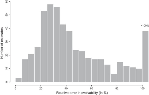
Distribution of relative errors in evolvability for 519 estimates from 40 studies. The median is 36% excluding 38 estimates with a relative error larger than 100% (see Supplement S6 for details). The relative error in the evolvability of gland area obtained from the diallel experiments were 18% in Tovar and 29% in Tulum. The relative error in evolvability is calculated as 100× the standard error in evolvability divided by the evolvability.

Open in new tab Download slide

Analyzing the temporal dynamics of our selection responses revealed that both direct and correlated responses were smaller than predicted, and that the direct responses were asymmetric with larger changes to decrease the gland size. While these responses individually fall within expected levels of uncertainty, their similarity in the two species suggests some violation of the assumptions of the Lande equation. We did find evidence for a Bulmer effect, that is, a decrease in additive variance due to linkage disequilibrium generated by selection, but this explained less than 10% of the difference between estimated and realized evolvabilities (Table 3).

Directional epistasis (i.e., when allele substitutions that increase a trait systematically increase or decrease effects of allele substitutions at other loci; Hansen and Wagner 2001) could explain the asymmetrical responses by increasing genetic variance in one direction and decreasing it in the other (Carter et al. 2005; Hansen et al. 2006; Pavlicev et al. 2010; Morrissey 2015). It would require strong epistasis to explain changes of this magnitude over so few generations, however, and more complex patterns of epistasis would be necessary to explain why the response is less than predicted in both directions of selection.

Other mechanisms such as natural selection counteracting the production of exaggerated traits or inbreeding depression could also generate asymmetrical responses (Frankham 1990; Walsh and Lynch 2018 chap. 18 for reviews). Inbreeding depression is unlikely to explain these patterns because we found no effects of selfing on blossom traits in these two species (Hansen et al. 2003a, Pélabon et al. 2004b, Opedal et al. 2015). Similarly, it is unlikely that natural selection would counteract a change in gland size in a greenhouse environment. Alternatively, an asymmetrical response could be generated by changes in the frequency of rare alleles with large effect (e.g., Frankham and Nurthen 1981; Kelly 2008). Stabilizing selection in natural populations may generate a negative relationship between allele frequency and effect size (Zhang and Hill 2005), but the asymmetry in the response observed here would imply a bias toward low frequency of alleles that decrease gland size. Although this could result from sustained directional selection to increase gland size, this scenario is not supported by observations of pollinator-mediated selection on gland area in several populations of D. scandens (Pérez-Barrales et al. 2013; Albertsen et al. 2021). Finally, we note that the asymmetry is more pronounced on an arithmetic scale and is thus not restricted to the log-scale we used.

The decrease of the correlated response of bract area observed in the Tulum population is also difficult to explain, because the underlying mechanism must change the additive genetic covariance of the traits more than it changes the additive variance in the selected trait. This is particularly puzzling in the light of our observation of little change in the phenotypic covariance.

Finally, the lower than expected response to selection may have resulted from an overestimation of additive genetic variance in the breeding experiments. Two possible causes of overestimation are epistatic variation and inbreeding among the parents used in the diallels. Neither of these mechanisms can explain the decline in the response only after the first generation, however. Furthermore, the similarity in the G-matrices estimated with or without the contribution of selfed individuals does not support the inbreeding hypothesis in the Tovar population, which was the one with the largest reduction of the observed responses.

Artificial selection has been instrumental in the development of the evolutionary theory from Darwin and onward (Robertson 1966; Wright 1977, Hill and Caballero 1992; Bell 2008), and it still provides valuable insights on the evolvability of quantitative traits (e.g., Beldade et al. 2002; Carlborg et al. 2006; Le Rouzic et al 2008; Pavlicev et al. 2010; Carter and Houle 2011; Hine et al. 2011; Bolstad et al. 2015; Sztepanacz and Blows 2017; Morgan et al. 2020). The lack of consideration of uncertainty in this type of experiment, however, has limited our ability to infer underlying genetic architecture from the discrepancies between observed and predicted responses. Despite the Lande equation being 40 years old, models that explicitly incorporate estimation of uncertainties in the prediction of evolutionary changes or allow analysis and interpretation of the selection-response dynamics in terms of genetic architecture are only starting to be developed (Le Rouzic et al. 2010, 2011; Stinchcombe et al. 2014). We argue that, with such models, a better and more systematic quantification of the imprecision associated with genetic parameters and their predictions will help us to better understand the limitations of the current approaches, and design experiments that will bring progress in understanding multivariate evolution. This should also help us in assessing predictability in eco-evolutionary dynamics.

AUTHOR CONTRIBUTIONS

C.P., T.F.H. and W.S.A. initiated the study. C.P. and E.A. collected the data. T.F.H. did the derivation on the prediction intervals in collaboration with A.L.R., G.H.B. and C.P. E.A., A.L.R., C.F., G.H.B. and C.P. performed the statistical analyses. C.P. did the literature search. C.P., E.A. and T.F.H. wrote the manuscript with contributions from all authors.

ACKNOWLEDGMENTS

We are grateful to Grete Rakvaag and Liv Antonsen for taking care of the plants during the selection experiment. We thank Michael B. Morrissey, three anonymous reviewers, and many people at the Centre for Biodiversity Dynamics (NTNU) for fruitful comments on earlier versions of this paper. Elena Albertsen was supported by the Research Council of Norway through its Centre of Excellence funding scheme, project no. 223257. We also thank the Norwegian Research Council (grant no. 196494 and 287214 to C.P. and 244139 to C.P. and A.L.R., and 275862 to G.H.B.) and the US National Science Foundation (grant nos. DEB-0444157 to T.F.H. and DEB-0444745 to W.S.A.) for financial support. C.P., T.F.H., A.L.R., and W.S.A. were hosted by the Center of Advanced Study (CAS) in Oslo during the writing of the paper.

DATA ARCHIVING

All the data and scripts that were used to conduct analyses and produce the figures are deposited in the Dryad Digital Repository: https://doi.org/10.5061/dryad.ns1rn8psz

CONFLICT OF INTEREST

The authors declare no conflict of interest.

Appendix 1 Drift variance under truncation selection

In this appendix, we derive equation 4 in the main text for the sampling variance in the mean breeding value of a quantitative trait after one generation of selection. We assume that exactly N_p parents are picked from a population of N individuals and then mated deterministically such that each parent produces exactly 2N/N_p offspring.

Let the phenotype of an offspring, i, be z_i = g_i + e_i, where g_i is the breeding value and e_i an environmental effect with mean zero and variance V_e. Let

\bar{g} = \frac{1}{N} \sum_{i} g_{i}

be the mean breeding value among the N offspring. To compute the variance in

\bar{g}

due to sampling we first write

V a r [\bar{g}] = E [V a r [\bar{g} | P]] + V a r [E [\bar{g} | P]],

where |P denotes conditioning on the N_p parents of the offspring. To simplify the computation, we now consider a single locus with two alleles, B and b, with frequencies p and q, and genotypic effects 2a, a, and 0 for BB, Bb, and bb, respectively. Assuming additivity and linkage equilibrium, the total genetic sampling variance will be the sum of the contribution from each locus. For each locus we have

E [\bar{g} | P] = 2 a p^{'},

V a r [\bar{g} | P] = a^{2} H^{'} / 2 N,

where p' and H' are the allele frequency and the heterozygosity among the parents. The first equation follows because each parent contributes exactly 2N/N_p alleles to the offspring's total of 2N alleles, and each of the 2Np' B-alleles contribute an effect a. To derive the second equation, note that every homozygous parent always contributes the same allele type to the offspring and thus no sampling variance. A heterozygote parent will contribute a variance of a²/4. There are H'N_p heterozygote parents, each being the parent of 2N/N_p alleles, so we get

\begin{matrix} Var [\bar{g} | P] & = & Var [\sum_{i} g_{i} / N | P] = \sum_{i} Var [g_{i} | P] / N^{2} \\ = & (a^{2} / 4) (H^{'} N_{p}) (2 N / N_{p}) / N^{2} = a^{2} H^{'} / 2 N . \end{matrix}

This is the variance due to random sampling of alleles from individual parents during mating. Putting the two equations together we get

V a r [\bar{g}] = (a^{2} / 2 N) E [H^{'}] + 4 a^{2} V a r [p^{'}] .

We now need to compute E[H'] and Var[p'] over samples of parents. We start with the case of no selection, as in our control lines. Here, parents are picked at random without replacement. The joint distribution of the numbers of BB homozygotes and Bb heterozygotes in the sample is multivariate hypergeometric with moments

\begin{matrix} E [N_{B B}^{'}] = N_{p} p_{B B}, \\ E [N_{B b}^{'}] = N_{p} p_{B b}, \\ V a r [N_{B B}^{'}] = N_{p} p_{B B} (1 - p_{B B}) (N - N_{p}) / (N - 1), \\ V a r [N_{B b}^{'}] = N_{p} p_{B b} (1 - p_{B b}) (N - N_{p}) / (N - 1), \\ C o v [N_{B B}^{'}, N_{B b}^{'}] = - N_{p} p_{B B} p_{B b} (N - N_{p}) / (N - 1), \end{matrix}

where p_BB and p_Bb are the frequencies of the two genotypes in the population before sampling. Using these moments, and p_BB = p² + Fpq and p_Bb = 2pq(1 - F), where F is the coefficient of inbreeding in the population before sampling, we derive

E [p^{'}] = p,

V a r [p^{'}] = \frac{p q (1 + F)}{2} \frac{N - N_{p}}{N_{p} (N - 1)},

E [H^{'}] = 2 p q (1 - F) .

This yields

\begin{matrix} V a r [\bar{g}] & = & \frac{p q a^{2} (1 - F)}{N} + \frac{2 p q a^{2} (1 + F) (N - N_{p})}{N_{p} (N - 1)} \\ = & 2 p q a^{2} (1 + F) (\frac{1 - F}{2 N (1 + F)} + \frac{N - N_{p}}{N_{p} (N - 1)}) \\ \approx & V_{A} (\frac{1}{N_{p}} - \frac{1 + 3 F}{2 N (1 + F)}), \end{matrix}

because the additive variance contributed by the locus is V_A = 2pqa²(1+F). If the population we sample from is in Hardy-Weinberg equilibrium (i.e., F = 0), this reduces to

V a r [\bar{g}] \approx V_{A} (1 / N_{p} - 1 / 2 N) .

To compute E[H'] and Var[p'] in the case of truncation selection, we need to make some approximations. The most important is that each locus has small effects such that we can ignore the effects of selection on the expected genotype frequencies. Hence, we assume E[N'_BB] = N_pp_BB and E[N'_Bb] = N_pp_Bb. We do, however, need to consider that individual parents differ in their probabilities of being selected. If we take the extreme case of a population in which all variance is additive genetic, then the probability of a given genotype being selected under truncation selection is either zero or one. This means that if we repeat the sampling, we will always pick exactly the same parents, and then Var[p'] = 0. If there are environmental sources of variation, then the probability of a given genotype being picked is uncertain and there will be sampling variance in p'. To quantify this, we need to compute the probability of picking a given genotype in the presence of environmental variance.

The number of BB individuals in the selected sample can be written as N'_BB = Σ_iy_i, where y_i is an indicator for whether individual i was included or not, and the sum is over all N_BB individuals that could be selected. The variance of this is

Var [N_{BB}^{'}] = Var [\sum_{i}^{N_{BB}} y_{i}] = \sum_{i}^{N_{BB}} Var [y_{i}] + \sum_{i}^{N_{BB}} \sum_{j \neq i}^{N_{BB}} Cov [y_{i}, y_{j}] .

The y_i are each sampled without replacement, and in each of the N_p sampling events this happens with a probability of w_i/N, where w_i is the relative fitness of the individual genotype. From this we can derive

\begin{matrix} V a r [y_{i}] & = & \frac{N_{p}}{N} w_{i} (1 - \frac{N_{p}}{N} w_{i}), \\ C o v {[y_{i}, y_{j}]}_{i \neq j} & = & - w_{i} w_{j} \frac{N_{p}}{N^{2}} (1 - \frac{(N_{p} - 1)}{2 N} (\frac{w_{i}}{1 - w_{i} / N} + \frac{w_{j}}{1 - w_{j} / N})) . \end{matrix}

Fitting this in yields

\begin{matrix} V a r [N {^{'}}_{B B}] & = & N_{p} P_{B B} (1 - P_{B B} - \frac{N_{p} - 1}{N} (1 + V a r [w]) \\ + P_{B B} (\frac{N_{p} - 1}{N}) E [\frac{w^{2}}{1 - w / N}] \\ - (\frac{N_{p} - 1}{N^{2}}) E [\frac{w^{3}}{1 - w / N}]), \end{matrix}

where variance and expectation are over relative fitness in the population before selection, and we have used E[w] = 1. To obtain an approximation in terms of the variance of fitness, we use a second-order Taylor approximation of the expectations around the mean relative fitness:

\begin{matrix} E [\frac{w^{2}}{1 - w / N}] & \approx & \frac{N}{N - 1} + \frac{N}{N - 1} (1 + \frac{{(N - 1)}^{4} (2 N - 1)}{N^{6}}) Var [w], \\ E [\frac{w^{3}}{1 - w / N}] & \approx & \frac{N}{N - 1} + (\frac{N (3 N - 2)}{{(N - 1)}^{3}}) Var [w] . \end{matrix}

Fitting in, collecting terms, and ignoring some terms of lower order in 1/N yields

V a r [N_{B B}^{'}] \approx N_{p} P_{B B} (1 - P_{B B}) (\frac{N - N_{p}}{N - 1}) (1 - (\frac{N_{p} - 1}{N - N_{p}}) V a r [w]) .

Hence, increasing variance in relative fitness, stronger selection will reduce the sampling variance from the expectation under random sampling. Eventually, when selection becomes deterministic, the sampling variance becomes zero. The variance in relative fitness under deterministic truncation selection is (N - N_p)/N_p. Using this in our equation, we find that the sampling variance is reduced with a factor 1/N_p relative to random sampling. Provided the number of selected parents is not extremely small, this is close to zero, and thus shows that the approximations are good even far from random sampling. Using the same approach, we compute

\begin{matrix} Var [N_{Bb}^{'}] & \approx & N_{p} P_{Bb} (1 - P_{Bb}) (\frac{N - N_{p}}{N - 1}) \\ \times (1 - (\frac{N_{p} - 1}{N - N_{p}}) Var [w]), \\ Cov [{N^{'}}_{BB}, {N^{'}}_{Bb}] & = & - N_{p} P_{BB} P_{Bb} (N - (N_{p} - 1) E [\frac{w^{2}}{1 - w / N}]) \\ \approx & - N_{p} P_{BB} P_{Bb} (\frac{N - N_{p}}{N - 1}) \\ \times (1 - (\frac{N_{p} - 1}{N - N_{p}}) Var [w]) . \end{matrix}

Using these we get

\begin{matrix} V a r [P^{'}] & = & V a r [\frac{N_{B B}^{'} + \frac{1}{2} N_{B b}^{'}}{N_{p}}] \\ \approx & \frac{p q (1 + F)}{2} \frac{N - N_{p}}{N_{p} (N - 1)} (1 - (\frac{N_{p} - 1}{N - N_{p}}) V a r [w]) . \end{matrix}

If we ignore the effects of selection on inbreeding and allele-frequency change, we can use this together with E[H'] = 2pq(1-F) to calculate

\begin{matrix} Var [\bar{g}] & = & \frac{a^{2} E [H^{'}]}{2 N} + 4 a^{2} Var [p^{'}] \\ \approx & \frac{pq a^{2} (1 - F)}{N} \\ + \frac{2 pq a^{2} (1 + F) (N - N_{p})}{N_{p} (N - 1)} (1 - (\frac{N_{p} - 1}{N - N_{p}}) Var [w]) \\ = & 2 pq a^{2} (1 + F) \\ \times (\frac{1 - F}{2 N (1 + F)} + \frac{N - N_{p}}{N_{p} (N - 1)} (1 - (\frac{N_{p} - 1}{N - N_{p}}) Var [w])) \\ \approx & V_{A} (\frac{1}{N_{p}} - \frac{1 + 3 F}{2 N (1 + F)} - \frac{Var [w]}{N}), \end{matrix}

where we have ignored terms of lower order in 1/N and 1/N_p. If the population we select from is in Hardy-Weinberg equilibrium, this reduces to

V a r [\bar{g}] \approx V_{A} (\frac{1}{N_{p}} - \frac{1 + 2 V a r [w]}{2 N}) .

Appendix 2 An approximation for the genotypic variance in fitness

While the variance in relative fitness of phenotypes under truncation selection is exactly (N - N_p)/N_p, what we need in the equations is the variance of the relative fitness of genotypes. This is not easily expressed in terms of observable population parameters. For our purpose, to make prediction intervals, we use a crude approximation based on dividing the population into three groups, one with breeding values for the selected trait at least one environmental standard deviation above the selection cutoff, k, one with breeding values at least one environmental standard deviation below the selection cutoff and one with breeding values in between. The two first groups we assign fitness of one and zero, respectively. For the intermediate group, we assign fitness equal to the mean fitness (N_p/N). We do this even if the fitness of a breeding value exactly at the cutoff is 1/2, because in our situation with N_p = N/4 most of the probability mass of the group will be below the cutoff. Using the mean fitness will also make the variance in fitness converge correctly to zero when the heritability goes to zero. We assume that the breeding values and the environmental effects of the selected trait are normally distributed. If F(g) is the cumulative normal probability function for the breeding values, we can write

\begin{matrix} F (k \pm \sqrt{V_{e}}) & = & \frac{1}{2} (1 + Erf [\frac{k - \bar{g} \pm \sqrt{V_{e}}}{\sqrt{2 V_{A}}}]) \\ = & \frac{1}{2} (1 + Erf [\frac{k - \bar{g}}{\sqrt{2 h^{2} V_{P}}} \pm \sqrt{\frac{1 - h^{2}}{2 h^{2}}}]), \end{matrix}

where

E r f [x] = \frac{2}{\sqrt{π}} \int_{0}^{x} e^{- t^{2}} d t

is the error function. The probability masses of the three categories are

1 - F (k + \sqrt{V_{e}})

⁠,

F (k - \sqrt{V_{e}})

⁠, and

F (k + \sqrt{V_{e}}) - F (k - \sqrt{V_{e}})

⁠, respectively, and using these we can write

\begin{matrix} V a r [w] & \approx & \frac{1}{E {[W]}^{2}} (1 - F (k + \sqrt{V_{e}}) \\ + {(E [W])}^{2} (F (k + \sqrt{V_{e}}) - F (k - \sqrt{V_{e}}))) - 1 \\ = & \frac{N^{2}}{2 N_{p}^{2}} (1 - (1 - \frac{N_{p}^{2}}{N^{2}}) E r f [\frac{k - g}{\sqrt{2 h^{2} V_{P}}} + \sqrt{\frac{1 - h^{2}}{2 h^{2}}}] \\ - \frac{N_{p}^{2}}{N^{2}} E r f [\frac{k - g}{\sqrt{2 h^{2} V_{P}}} - \sqrt{\frac{1 - h^{2}}{2 h^{2}}}]) - 1, \end{matrix}

where W is absolute fitness. From the assumed normal distribution of the breeding values we have

F (k) = \frac{N - N_{p}}{N}

which yields

k - \bar{g} = \sqrt{V_{A}} F^{- 1} (\frac{N - N_{p}}{N}) = \sqrt{2 V_{A}} Er f^{- 1} [2 (\frac{N - N_{p}}{N}) - 1],

where

\sqrt{2} E r f^{- 1} [x]

is the probit function. Fitting this in we get

V a r [w] \approx \frac{N^{2} - 2 N_{p}^{2}}{2 N_{P}^{2}}

- (\frac{N^{2} - 2 N_{p}^{2}}{2 N_{p}^{2}}) E r f [E r f^{- 1} [2 (\frac{N - N_{p}}{N}) - 1] + \sqrt{\frac{1 - h^{2}}{2 h^{2}}}]

- \frac{1}{2} E r f [E r f^{- 1} [2 (\frac{N - N_{p}}{N}) - 1] - \sqrt{\frac{1 - h^{2}}{2 h^{2}}}],

which can be computed from the heritability of the selected trait. This approximation gives the correct values of (N - N_p)/N_p when h² = 1 and zero when h² = 0. We used this variance computed from the estimated heritability of the selected trait in equation 7 to make prediction intervals.

LITERATURE CITED

Albertsen

Ø. H.

Opedal

G. H.

Bolstad

Pérez-Barrales

T. F.

Hansen

Pélabon

and

W. S.

Armbruster

2021

Using ecological context to interpret spatiotemporal variation in natural selection

Evolution

294

–

309

Month:	Total Views:
December 2022	3
January 2023	5
February 2023	16
March 2023	11
April 2023	18
May 2023	6
June 2023	7
July 2023	8
August 2023	29
September 2023	17
October 2023	19
November 2023	10
December 2023	26
January 2024	25
February 2024	43
March 2024	33
April 2024	19
May 2024	35
June 2024	19
July 2024	24
August 2024	10
September 2024	12
October 2024	18
November 2024	22
December 2024	12
January 2025	17
February 2025	27
March 2025	39
April 2025	30
May 2025	12

Article Contents

Quantitative assessment of observed versus predicted responses to selection Open Access

Abstract

Theory: Prediction Error in Artificial Selection

Materials and Methods

STUDY SPECIES AND TRAIT MEASUREMENTS

DIALLEL EXPERIMENT

SELECTION EXPERIMENT

STATISTICAL ANALYSES

Genetic parameters from the diallel experiment

Comparing observed and predicted response to selection

Analyzing the temporal dynamics of the responses to selection

Results

GENETIC VARIATION AND EVOLVABILITY

DIRECT RESPONSE TO SELECTION

CORRELATED RESPONSE TO SELECTION

Discussion

AUTHOR CONTRIBUTIONS

ACKNOWLEDGMENTS

DATA ARCHIVING

CONFLICT OF INTEREST

Appendix 1 Drift variance under truncation selection

Appendix 2 An approximation for the genotypic variance in fitness

LITERATURE CITED

Supplementary data

Citations

Views

Altmetric

Email alerts

Citing articles via

Latest

Most Read

Most Cited

This Feature Is Available To Subscribers Only

Quantitative assessment of observed versus predicted responses to selection