


Abstract
Additive genetic variance in a trait reflects its potential to respond to selection, which is key for adaptive evolution in the wild. Social interactions contribute to this genetic variation through indirect genetic effects—the effect of an individual's genotype on the expression of a trait in a conspecific. However, our understanding of the evolutionary importance of indirect genetic effects in the wild and of their strength relative to direct genetic effects is limited. In this study, we assessed how indirect genetic effects contribute to genetic variation of behavioral, morphological, and life-history traits in a wild Eastern chipmunk population. We also compared the contribution of direct and indirect genetic effects to traits evolvabilities and related these effects to selection strength across traits. We implemented a novel approach integrating the spatial structure of social interactions in quantitative genetic analyses, and supported the reliability of our results with power analyses. We found indirect genetic effects for trappability and relative fecundity, little direct genetic effects in all traits and a large role for direct and indirect permanent environmental effects. Our study highlights the potential evolutionary role of social permanent environmental effects in shaping phenotypes of conspecifics through adaptive phenotypic plasticity.
Social interactions are ubiquitous in nature: courtship, competition, communication, and cooperation can only be expressed during direct or delayed interactions with conspecifics (Székely et al. 2010; Westneat and Fox 2010). Through these interactions, the phenotype of an individual, and thus, its underlying genotype, can affect the phenotype of other individuals and impact their fitness. The influence of an individual's genotype on the expression of a trait in a conspecific is termed as indirect genetic effects (Moore et al. 1997; Wolf et al. 1998, Wolf et al. 1999; McGlothlin et al. 2010). For example, in common gulls (Larus canus), male genotypes affect the seasonal timing of egg-laying date of their partners (Brommer and Rattiste 2008). Indirect genetic effects differ from any other environmental effects, because the social environment can itself evolve and, thus, contributes to the evolutionary response to selection (Wolf et al. 1998; Wolf et al. 1999; McGlothlin et al. 2010). Traditional quantitative genetic models of evolution mainly consider direct genetic effects of an individual's genotype on its phenotype as a source of genetic variation, assuming a null contribution of the environment to the genetic variation. The importance of indirect genetic effects has long been recognized by quantitative geneticists interested in how the social environment affects responses to artificial selection in domestic animals (Griffing 1967; Bijma et al. 2007a,b; Bijma and Wade 2008). Recent evidence suggests that indirect genetic effects may be widespread in natural populations (Bailey et al. 2018). For example, parental effects—a widely studied indirect genetic effect—are prevalent in many species (McAdam et al. 2014). Studying the genetic basis of traits should, thus, include the estimation of indirect genetic effects to assess the extent of conspecifics effects on genetic variation and their role in the evolution of these traits.
Quantitative genetic theory shows that indirect genetic effects can have major evolutionary consequences when they are correlated with direct genetic effects (Moore et al. 1997; Wolf et al. 1998; Bijma and Wade 2008). Negative direct–indirect genetic correlations can impose major evolutionary constraints by reducing the total heritable variation of a trait (Wolf et al. 1998; Bijma 2011). In contrast, positive direct–indirect genetic correlations provide a source of additional genetic variation to the trait, and accelerate its response to directional selection (Moore et al. 1997; Wilson et al. 2009; Bijma 2011, 2014; Santostefano et al. 2017). Yet, apart from a few studies (e.g., Brommer and Rattiste 2008; Teplitsky et al. 2010; Wilson et al. 2011; Sartori and Mantovani 2012; Reid et al. 2014; Adams et al. 2015; Germain et al. 2016; Fisher et al. 2019; Evans et al. 2020), empirical estimates of indirect genetic effects, other than maternal effects, in wild populations are still rare (McAdam et al. 2014). Such studies in nature are difficult because they require long-term population monitoring, parentage analyses, and large data sets (Charmantier et al. 2014). However, studies in wild populations have the advantage of using traits expressed in a natural and biologically meaningful context (Niemelä and Dingemanse 2014), and will help us understand the evolutionary importance of indirect genetic effects (Kruuk and Wilson 2018).
Indirect genetic effects have been found across several types of traits (Ellen et al. 2014; McAdam et al. 2014; Bailey et al. 2018; Fisher and McAdam 2019). However, at the moment, a theoretical framework is lacking to predict whether the strength of these effects should vary depending on the trait and on the ecological conditions. Behavioral phenotypes can change quickly through phenotypic plasticity in response to changes in environmental conditions—including the social environment—and are highly context dependent (Bailey et al. 2018). Behavioral ecologists are starting to apply the indirect genetic effects framework in a variety of contexts, but models suggest that they should matter in sexual selection, sexual conflict, agonistic interactions, and the evolution of sociality (Bailey et al. 2018). Dingemanse and Araya-Ajoy (2015) have advocated incorporating the estimation of indirect genetic effects in studies on behavioral variation, since social interactions might generate among-individual variation in behavior (personality), within-individual variation (plasticity), and individual differences in social responsiveness (see also Montiglio et al. 2013). Indirect genetic effects could also impact traits related to competition, such as growth or resource-dependent life-history traits, that are not social traits per se (Wilson 2014), but still depend on phenotypes of conspecifics. For example, trees vary in their genetic effects on bark diameter growth of their neighbors, where fast-growing trees reduce the growth of neighbors (Costa E Silva et al. 2013). Individuals can also influence each other's fitness, and therefore, indirect genetic effects should also impact fitness traits (see Fisher and McAdam 2019 for an extensive treatment of this topic), and could generate social selection (Wolf et al. 1999) or group selection (Goodnight et al. 1992). However, until now, the relative proportion of phenotypic variance explained by direct or indirect genetic effects in different types of traits, and the importance of indirect genetic effects to traits evolvability, is still unknown (Bailey et al. 2018).
The complexity of natural social structures complicates the estimation of indirect genetic effect in the wild. For example, several individuals with different degrees of relatedness often interact. Furthermore, limited dispersal, habitat heterogeneity, and resource availability should influence the spatial distribution of territorial individuals and, thus, their social relationships (Cote et al. 2010; Farine and Sheldon 2015; Dubuc-Messier et al. 2012). Therefore, another challenge is to integrate the spatial and social structure of a population to “scale” the intensity of indirect genetic effects. This aim can be achieved by adapting methods developed in forestry studies, in which estimates are weighted by the distance between trees, reflecting variation in the intensity of competition (Cappa and Cantet 2008; Costa e Silva and Kerr 2013). In territorial animals, a competition-intensity factor can be derived from the distance between home-range centers (Fisher et al. 2019), from estimates of resource use overlap or measures of social interaction frequency based on social networks (Wey et al. 2008; Sih et al. 2009; Wilson 2014). Additionally, this method allows explicit modelling of the monogenetic component (i.e., permanent environmental) of indirect effects, which may otherwise bias estimates of indirect genetic variance (Costa e Silva and Kerr 2013; Wilson 2014). Including multiple interactions and the spatial distribution of phenotypes can, therefore, improve our characterization of indirect genetic effects in wild populations.
In this study, we used a dataset and a pedigree, from a long-term study between 2005 and 2018 on a wild population of Eastern chipmunks (Tamias striatus) in southern Québec (Canada), to estimate direct and indirect genetic effects on four behavioral traits (exploration, docility, trappability, core range area), a morphological trait (body mass), and three life-history traits (age at sexual maturity, lifespan, relative fecundity). Chipmunks use underground burrows, in which they hoard seeds produced by masting deciduous trees (Snyder 1982). Home ranges can overlap, but individuals aggressively defend the core area around their burrow where they spend most of their time above ground (Elliot 1978). Thus, indirect genetic effects have the potential to act on competition and resource acquisition-based traits such as body mass and home range area. A previous study in this population showed that social interactions between neighbors can generate social selection on docility and body mass, where neighbors’ traits affect an individual's fitness (Santostefano et al. 2019). Therefore, we may also expect neighbors’ genotypes to affect several traits through indirect genetic effects in this population (McGlothlin et al. 2010). As a first objective, we thus (i) modeled indirect genetic effects, by scaling the strength of interactions based on the intensity of association with multiple neighbours.
Second, we (ii) assessed the contribution of direct and indirect genetic effects to the evolutionary potential of different trait types. Heritability (h2) has traditionally been used as an index of the evolutionary potential of a trait. However, values of heritability (and the corresponding ige2 for indirect genetic effects) depend on other sources of variation in the measured trait and thus inform us on the magnitude of indirect and genetic effects relative to other components (Houle 1992; Hansen et al. 2011). Instead, mean-standardized measures of a trait's additive genetic variance, such as the coefficient of additive genetic variation (CVa) and its squared version (Ia), provide more appropriate indices of that evolutionary potential, or evolvability (Houle 1992; Hansen et al. 2011; Garcia-Gonzalez et al. 2012; Postma 2014). Cva and Ia are independent of other sources of variance (e.g., environmental variance), and this makes them suitable for comparisons in terms of absolute evolutionary potential. Life-history traits, and more particularly fitness components, have low heritabilities but high evolvabilities, which on a variance-standardized scale gets masked by the very high levels of environmental (or possibly nonadditive genetic) variation in such traits (Price and Schluter 1991; Houle 1992; Kruuk et al. 2000; Hansen et al. 2011). We, thus, compared the importance of direct and indirect genetic effects on different traits by examining both their CVs and Is (Houle 1992; Hansen et al. 2011).
The correlation between the strength of selection and additive genetic variance could also affect the rate of evolutionary change in quantitative traits (Wood and Brodie 2016). Traits more tightly related to fitness, such as fecundity and viability, should be under stronger selection than morphological and physiological traits, and therefore, have a lower additive genetic variance (Mousseau and Roff 1987; Falconer and Mackay 1996; Stirling et al. 2002; Morrissey 2014). We can, thus, expect a negative correlation between a trait's additive genetic variance and the strength of selection pressures acting on it (which is measured by estimating the covariance with lifetime reproductive success, LRS). Since indirect genetic effects are also a source of heritable variation, we wanted to explore their relationship with selection strength, although we could not find any predictions on its sign in the literature. Thus, as an exploratory objective, we (iii) compared across traits the correlation between both direct and indirect genetic effect variances of a trait and the strength of selection acting on it.
Estimating indirect genetic effects from an animal model can be data hungry, and simulation analyses are necessary to test the limits of a particular dataset, pedigree, or model (Morrissey et al. 2007; Wilson et al. 2010; Bourret and Garant 2017). Simulations can provide information on the power to detect an effect and on the accuracy and precision of the estimates. Thus, as our last objective, (iv) we used simulated data to assess precision and accuracy of quantitative genetic estimates, including indirect genetic effects, as well as the power of detecting these variance components.
Materials and Methods
STUDY POPULATION
We monitored a wild population of Eastern chipmunks in southern Québec, Canada (45°06′ N; 72°25′ W). The habitat consisted in a deciduous forest dominated by American beech trees (Fagus grandifolia), red maples (Acer rubrum), and sugar maples (Acer saccharum). Eastern chipmunks are small forest-dwelling mammals that consume and hoard seeds produced by masting trees (Snyder 1982). Chipmunks are diurnal and display variable levels of above-ground activity in spring and summer, but they overwinter with little to no above-ground activity (Munro et al. 2008), and enter torpor for a large part of the winter (Landry-Cuerrier et al. 2008; Dammhahn et al. 2016). In southern Québec, they can reproduce during two distinct seasons: early spring or summer—in phase with the American beech masting cycle (Bergeron et al. 2011a,b). Beech mast occurs in the fall about once every other year. Summer reproduction happens before a masting event, and spring reproduction always follows a fall masting event. Chipmunks do not reproduce in the summer preceding or the spring following a nonmasting fall (Bergeron et al. 2011a,b, 2013). Juveniles spend the first few weeks after birth in their mother's burrow. They leave the maternal burrow within two weeks following the first emergence from the burrow and disperse to settle in vacant burrows (Elliot 1978). Males disperse further than females, and both dispersal and genetic structure change according to environmental conditions (Dubuc-Messier et al. 2012). Eastern chipmunks have a promiscuous mating system and females produce litters of 2 to 5 offspring. Multiple paternity is common and varies from 25% (spring reproductions) to 100% (summer reproductions; Bergeron et al. 2011c). Chipmunks live 30 months on average (Bergeron et al. 2011b).
DATA COLLECTION OVERVIEW
We monitored chipmunks on four study sites: Site 1 (2005-2010), and sites 2, 3, and 4 (2012-2018). All the sites were within 10 km of each other, the habitat was similar between all the sites (St-Hilaire et al. 2017) and there is no significant genetic population structuring at this scale, as previously shown in Chambers and Garant (2010). All sites consisted of a grid marked with permanent stakes every 20 m, where traps were placed every 40 m. Site 1 was 25 ha for 228 trap locations (Bergeron et al. 2011b), whereas sites 2, 3, and 4, were respectively 6.76 ha, 6.76 ha, and 3.24 ha, with 98, 98, and 50 trap locations, respectively. We trapped chipmunks daily from May to October using Longworth traps checked at 2-hour intervals, from 8 a.m. until dusk. At each capture, we aged and sexed individuals (Careau et al. 2010); we classified as adults individuals that were born in the spring and the summer and were captured the following spring. We also weighted individuals to the nearest 1 g with a Pesola balance and uniquely marked them with ear tags and pit-tagged them for individual identification. At first capture, we sampled ear tissue from each individual and kept in 95% ethanol until genetic analyses (Bergeron et al. 2011c). We divided each year into two periods: spring (May–July) and summer (August–October).
BEHAVIORAL TESTS
Upon each capture, we transferred the chipmunk from the trap to a mesh handling bag and measured the number of seconds spent immobile for one minute as a measure of docility (Martin and Réale 2008). We quantified responses to a novel environment (“exploration”) following the standard open field (OF) test for rodents (Réale et al. 2007; Martin and Réale 2008; Montiglio et al. 2010). The OF arena was a rectangular wooden box with a transparent Plexiglas lid, with a camera mounted on a tripod above for recording. After capture, chipmunks were placed at the entrance of the exploration arena and their movements recorded for 90 s (see Montiglio et al. 2010, 2012 for details). Exploration levels were quantified as the number of times a chipmunk crossed a superimposed digital grid in the video analysis (following Montiglio et al. 2010).
LIFE-HISTORY TRAITS
We used three life-history traits. We measured relative seasonal reproductive success as the number of offspring assigned to an individual for each season, divided by population mean per season. Individuals that lived near the boundaries of the grid may have produced offspring outside the grid. However, preliminary analyses showed that the spatial distribution of phenotypes is not linked to the position of territories on the periphery of the grid. In our previous study (Santostefano et al. 2019), we checked for any edge effect on selection estimates by excluding individuals whose core range centroid fell in the two outer trapping lines closer to the edge in a further analysis. This reduced the area and also the number of individuals by 30%. Results on selection gradients were qualitatively similar. There is, thus, a relatively low possibility that edge effects could bias our estimates of indirect genetic effects. We measured lifespan as the minimum number of days that an individual lived (from emergence from the maternal burrow as a juvenile until the last capture); to reduce data censoring issues, we assigned NAs for lifespan to all the individuals that were still alive the year following the last year of data used in this study (2010 for site 1, 2019 for sites 2–4; N = 248, 8% of the total number of individuals recorded in the study). Redoing the analyses including these individuals did not change qualitatively the variance component estimates (results not shown). We measured age at sexual maturity as the number of days after emergence at which the individual displayed the first signs of reproduction: this is based on the presence of darkened scrotum for males or developed mammae for females (Careau et al. 2010). For individuals that were captured as adults, we used the latest emergence date on the site in the previous year to estimate the minimum lifespan and minimum age at sexual maturity.
SPATIAL MEASUREMENTS
The core range represents the area within the home range that an individual uses more frequently, and likely contains its refuges and its most dependable food sources (Burt 1943). We derived core range measurements based on individual trapping data for each season separately. We used grid coordinates for each capture to estimate the 50% kernel density function in the R package adehabitatHR (Calenge 2006), corresponding to the core range. To estimate the kernel function, we retained only individuals with more than five captures per season. This method excludes individuals with a low recapture rate, individuals whose territory is mostly outside the grid, and vagrant individuals; this ensures that we retain information only on the resident population and helps reduce a possible edge effect. Therefore, we believe we minimized the effects of peripheral position on quantitative genetic estimates, but we acknowledge that they may be present due to the nature of studies on wild populations and uncertainty on parentage assignment. We also used the coordinates of the centroids’ vertices to estimate the distance between territories; when this information was not available, we used an individual's burrow location from telemetry data as the center of its territory. This allowed us to estimate the pairwise distances between all the residents on the site for each season separately, which are used as intensity of association factors between neighbors to scale indirect genetic effects. Last, individual trapping information was also used to define the trait “trappability” as the number of times an individual was captured during a season.
GENETIC ANALYSES
We used parentage assignment to estimate individual reproductive success in each season and to build the pedigree for the animal model analyses. We extracted DNA from ear tissue and genotyped individuals at 11 polymorphic microsatellite loci for site 1 and 14 additional microsatellites for sites 2,3, and 4, using protocols developed for this species (see Chambers and Garant 2010; Vandal et al. 2020 for details). We first assigned maternity when we trapped juveniles at their emergence from the burrow. We then confirmed maternity using genetic information and a likelihood approach set at 95% confidence level with the software CERVUS (Kalinowski et al. 2007; see Bergeron et al. 2011c for details). We then assigned paternity to the juveniles using the same genetic assignment procedure, but by also including the assigned mother. For summer reproductive seasons, we consider as putative parents all the adults captured on a grid between early May and late July. For spring reproductive seasons, putative parents were all the individuals either captured on the grid the year before or adults captured in May or June of the year. The number of records in the pedigree is 1540, with 490 maternities and 398 paternities. The total number of full sibs is 102, while maternal and paternal sibs are 1039 and 513, respectively. The number of grandmothers is 171 (of which 148 maternal and 23 paternal), whereas the number of grandfathers is 119 (of which 104 maternal and 15 paternal). Maximum pedigree depth is four generations, and minimum depth is zero generations. Average relatedness across the whole pedigree is 0.001.
STATISTICAL ANALYSES
Depending on the trait, we organized our data in three datasets with different structures: (1) traits with repeated measures per individual per season (exploration, docility, body mass); (2) traits with one measure per individual per season (relative fecundity, core range area, trappability); (3) traits with one measure per individual per lifetime (longevity, age at sexual maturation). Data analyses for all three datasets are largely similar except for a few differences in fixed and random effect structure (see details below).
We analyzed the data using univariate mixed-effect animal models (Kruuk 2004; Wilson et al. 2010) that included the (additive) relatedness matrix calculated from the pedigree. For each trait, we partitioned the total phenotypic variance () into its underlying variance components: direct (additive) genetic (), direct permanent environmental () effects, indirect genetic (), and indirect permanent environmental effects (), season-year (), and residual variance (). We estimated the proportional contribution of each variance estimate by dividing it by the total phenotypic variance not attributable to fixed effects to facilitate comparison of variance components across traits: Direct heritability ( ), indirect genetic effects ( ), and the proportional contribution of, , relative to . Note that it was impossible to separate residual from permanent environmental effects in models using dataset #3. We also included in these models season-year of birth as a random effect instead of season-year. We note that limitations of the available data prevented us from including maternal or common environmental effects as additional random effects. A glossary of abbreviations used in the text is presented in Table 1.
To statistically control for sources of variation in traits not directly relevant to our hypotheses, we included the following fixed effects: sex, season of data collection (spring or summer, datasets 1 and 2 only), age (datasets 1 and 2 only), age2 (datasets 1 and 2 only), site (four levels), population density (per season-year combination), day of the year (dataset 1 only), season of birth (i.e., birth cohort, spring or summer). Effects of season, site, and density are partially nested (e.g., season-year is the same for all sites, but density by season-year is different by site). Testing for differences between sites or season-years was not our objective, and therefore, fitting them both allowed us to control for site and year differences even if they partially overlap. All models were fitted using restricted maximum likelihood; dependent variables were mean centered. We also ran the final complete model for each trait without centering and standardizing variances to extract the raw variance components necessary to estimate mean-standardized variances for direct and indirect genetic effects. Throughout, we assumed a Gaussian error distribution, which was confirmed for all response variables after visual inspection of model residuals.
We tested model fixed effects using conditional F-tests with denominator degrees of freedom (df) estimated from the algebraic algorithm in ASReml 4.1 (Gilmour et al. 2015). We used a hierarchical stepwise forward approach (Nussey et al. 2007; Wilson et al. 2010) to evaluate the statistical significance of random effects by likelihood ratio tests (LRTs). For datasets 1 and 2, we started with a phenotypic model that contained only fixed effects and residual variance (Model 1). We then added season-year effect variance (Model 2). We estimated among-(focal)individual variance in the trait () by fitting individual identity (Model 3). We then partitioned this variance into direct genetic () and permanent environmental variance by linking individuals to pedigree information (Model 4). We repeated that structure for the social environment effects and tested for differences among social partners by fitting social partner identity (Model 5). We then partitioned this variance into indirect genetic (i.e., ) and permanent environmental variance () by including pedigree information (Model 6). For dataset 3, we used the same approach and started with a phenotypic model that contained only fixed effects and residual variance (Model 1), then tested for season-year of birth effects (Model 2). We then added estimates of genetic variance (Model 3) and social partner variance (Model 4).
We tested each random effect using a LRT = 2(logL2-logL1), where logL1 and logL2 are the log-likelihood of the model including and excluding the random effect, respectively. LRT is assumed to follow a χ 2-distribution (Shaw 1991). Variances are bound to be positive, therefore, in testing them we applied the LRT assuming (for testing a single variance component) the distribution of the LRT statistic is an equal mixture of χ20 and χ21 (Self and Liang 1987; Visscher 2006). When a correlation was also modeled between focal and social variance components (models 4 and 6 for datasets 1 and 2), a variance and covariance were tested together and, therefore, over an equal mixture of χ21 and χ22.
SOCIAL EFFECTS
To model social effects, we followed methods developed in forestry (Cappa and Cantet 2008; Costa e Silva and Kerr 2013) and applied to wild animals in Fisher et al. (2019). We included the identities of the four closest chipmunks as four random effects in the models, which were assumed to come from the same distribution, with a mean of zero and a single variance: this allowed us to estimate a single indirect (genetic or permanent environmental) effect. We chose the four nearest neighbors based on the distance between home-range centers of all the residents on a site within a season. We chose the arbitrary number of four neighbors by calculating the average number of individuals with overlapping core ranges, i.e., individuals that are likely interacting directly (based on data from Santostefano et al. 2019; across all seasons Mean 4.205, SD = 3.575, N = 603; see Fisher et al. 2019 for discussions on choosing different numbers of neighbors). We associated each neighbor (j) of each focal individual (i) with an intensity-of-association factor (fij). This allowed the indirect effect of each neighbor j experienced by i to be mediated by their spatial proximity, with fij = 1/(1 + distance), where distance was the Euclidean distance between the center of individuals’ home ranges. This value is bounded between 0 and 1, with low values representing individuals that were far apart and high values representing individuals that were close. To weigh the strength of indirect effects, we replaced all 1s in the indirect effect design matrix with these terms (Muir 2005; Cappa and Cantet 2008; Fisher et al. 2019). These terms link and scale indirect effects of individuals with the phenotypes of the focal individuals. Variance components for indirect genetic and indirect permanent environmental effects are then calculated following Figure 1 in Bijma (2011) and Costa E Silva et al. (2013) by multiplying the estimated indirect variance component by the number of neighbors and the squared mean of the association factor .
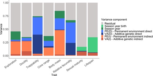
Proportion of phenotypic variance estimated from animal models (see Main text) in behaviors, morphology, and life-history traits, after accounting for variance explained by fixed effects. Note that for sexual maturity and life span, season-year of birth is fitted instead of season-year, and permanent environmental effects are not estimated.
where a trait y measured on individual i at time t results from the population mean accounting for the fixed effects μFi, a direct additive genetic effect , a direct, permanent environmental effect , the indirect additive genetic and permanent environmental effects of the four neighbors j interacting with i, a season-year term , and an individual residual term . A represents the matrix of relatedness, whereas PE is the matrix of identity for individual values. For dataset 3, was replaced by a season-year of birth term , whereas the permanent environmental effects and were not included.
COMPARING DIRECT AND INDIRECT GENETIC EFFECTS
To evaluate the contribution of direct and indirect genetic effects to the evolvability of different types of traits (Hansen et al. 2011; Bailey et al. 2018), we used two mean-standardized measures: the coefficient of additive genetic variation (CVa) and its squared version (Ia) (Houle 1992; Hansen et al. 2011), as well as their indirect genetic effects counterparts (CVige and Iige). While CV has been more widely used, I has a more straightforward interpretation as the expected percent change in a trait under a unit strength of selection (Hansen et al. 2011). To do so, we used raw variance estimates from the same set of models, without centering and standardizing the traits.
The correlation between the strength of selection and additive (direct and indirect) genetic variance could also contribute to the rate of evolutionary change in quantitative traits. We, thus, qualitatively compared the correlations between VAD and its association with fitness, with VAI and its association with fitness, across traits. To do so, we estimated the phenotypic covariance between each trait and LRS (total number of offspring) as a measure of selection strength, and correlated this to VAD and VAI in each trait. LRS was calculated as the total number of offspring produced by an individual in its lifetime; to avoid data censoring issues, we assigned NA to those still alive at the end of the study (see details above for lifespan).
SIMULATION ANALYSES
Some tools are available to perform simulation analyses in natural populations, including traits heritability (e.g., the package pedantics, Morrissey and Wilson 2010), but no universal tools exist to simulate indirect genetic effects. A handful of studies so far have simulated them with custom-built programs, or adapting existing ones for their needs (e.g., see McGlothlin and Brodie 2009, Bijma 2010, Lipschutz-Powell et al. 2012, Khaw et al. 2014). Here, we adapted the package pedantics to obtain simulations based on our dataset structure.
All variance components were normally distributed around 0. was always set to 1, and thus, was equal to the unexplained variance (i.e., ). As in equation (1), indirect genetic effects (i.e., and ) corresponded to the sum of the four neighbors. By default, all variance components, except , were set to 0.1. We then increased each variance component from 0.1 to 0.5 by a step of 0.1, while other variance components were kept fixed to 0.1 and the covariance terms were fixed to 0. Additionally, we then varied each covariance component (genetic, , and permanent environmental, ) by increasing the correlation terms from 0.2 to 0.8 by steps of 0.2, while keeping all variance components fixed to 0.1. The simulation of dataset #3 excluded direct and indirect permanent environmental variances (i.e., and ). All simulations were performed with a custom code in R version 3.6.1, and breeding values (i.e., direct and indirect genetic effects) were simulated with the package pedantics (Morrissey and Wilson 2009) and our empirical pedigrees. Each simulation scenario was repeated 100 times and analyses were performed with ASReml (version 4.1).
For each simulation scenario, we estimated the power of significantly detecting a specific variance component using the “rule of thumb” approach for which significance is assumed when estimates are two times larger than their standard error (Wilson et al. 2011; Bourret and Garant 2017). We also calculated the root mean square error and the imprecision (standard deviation of estimated values).
Results
ADDITIVE GENETIC AND DIRECT PERMANENT ENVIRONMENTAL EFFECTS
All traits were repeatable (where repeatability = Vindividual/VP) (Table 2), with individual repeatability estimates ranging from very low values for life-history traits (R = 0.03 ± 0.02 SE) to moderate for behaviors (R = 0.20 ± 0.2 SE to 0.29 ± 0.01 SE), and higher for body mass (R = 0.64 ± 0.03 SE). Traits showed little additive genetic variance and, thus, low heritabilities (0.00 ± 0.00 SE < h2 < 0.08 ± 0.03 SE), and docility was the only significantly heritable trait (h2 = 0.08 ± 0.03 SE). Direct permanent environmental effects (PED) varied considerably from one trait to another, representing most of the among-individual variation (Table 2, Fig. 1). PEDs were negligible for relative fecundity, small to moderate for behaviors (0.02 ± 0.01 SE to 0.24 ± 0.08 SE), and substantial in body mass (0.46 ± 0.03 SE).
Glossary of the abbreviations used in the text
| Abbreviation | Description |
|---|---|
| VP | Total phenotypic variance |
| VAD | Direct additive genetic variance |
| VPED | Direct permanent environmental variance |
| VAI | Indirect additive genetic variance (also known as IGEs) |
| VPEI | Indirect permanent environmental variance |
| VSY | Season-year variance |
| Ve | Residual variance |
| COVA | Additive genetic covariance |
| COVPE | Permanent environmental covariance |
| r AD,AI | Additive genetic correlation |
| r PED,PEI | Permanent environmental correlation |
| Vindividual | Among individual variance |
| Vsocial | Among individual social variance |
| h2 | Heritability; VAD/VP |
| ige2 | VAI/VP |
| CVa | Coefficient of additive genetic variation |
| Ia | VAD/m2 |
| CVige | Coefficient of indirect additive genetic variation |
| Iige | VAI/m2 |
Results of mixed animal models of increasing complexity in random effect structure fitted to partition variation in behaviors (a), morphology (b), and life-history (c) traits
| Variance/VP (SE) | Correlation | ||||||||||||||
|---|---|---|---|---|---|---|---|---|---|---|---|---|---|---|---|
| a. Trait | Model | Individual | VAD (h2) | VPED | Social | VAI (ige2) | VPEI | Season_year | Residual | r AD,AI | r PED, PEI | Loglik | Χ² | df | P |
| Exploration | 1. | – | – | – | – | – | – | – | – | – | – | −407.996 | – | – | – |
| 2. | – | – | – | – | – | – | 0.153 (0.059) | 0.847 (0.059) | – | – | −373.516 | 68.96 | 0/1 | <0.001 | |
| 3. | 0.257 (0.061) | – | – | – | – | – | 0.160 (0.060) | 0.582 (0.072) | – | – | −368.512 | 10.008 | 0/1 | <0.001 | |
| 4. | – | 0.074 (0.064) | 0.179 (0.085) | – | – | – | 0.160 (0.060) | 0.585 (0.072) | – | – | −367.751 | 1.522 | 0/1 | 0.11 | |
| 5. | – | 0.043 (0.063) | 0.233 (0.085) | 0.021 (0.040) | – | – | 0.158 (0.060) | 0.543 (0.075) | – | – | −365.391 | 4.72 | 1/2 | 0.04 | |
| 6. | – | 0.029 (0.061) | 0.242 (0.085) | – | 0.007 (0.084) | 0.023 (0.101) | 0.157 (0.060) | 0.539 (0.076) | 0.469 (6.542) | 0.789 (3.349) | −366.020 | −1.258 | 1/2 | 1.5 | |
| Docility | 1. | – | – | – | – | – | – | – | – | – | – | −5732.98 | – | – | – |
| 2. | – | – | – | – | – | – | 0.016 (0.006) | 0.983 (0.006) | – | – | −5678.03 | 109.9 | 0/1 | <0.001 | |
| 3. | 0.294 (0.012) | – | – | – | – | – | 0.019 (0.007) | 0.685 (0.013) | – | – | −4218.37 | 2919.32 | 0/1 | <0.001 | |
| 4. | – | 0.103 (0.031) | 0.191 (0.030) | – | – | – | 0.022 (0.008) | 0.682 (0.013) | – | – | −4211.57 | 13.6 | 0/1 | <0.001 | |
| 5. | – | 0.089 (0.030) | 0.188 (0.030) | 0.054 (0.009) | – | – | 0.016 (0.006) | 0.651 (0.013) | – | – | −4168.80 | 85.54 | 1/2 | <0.001 | |
| 6. | – | 0.084 (0.030) | 0.191 (0.030) | – | 0.005 (0.023) | 0.055 (0.025) | 0.016 (0.006) | 0.647 (0.013) | -0.799 (1.584) | 0.190 (0.211) | −4168.50 | 0.6 | 1/2 | 0.657 | |
| Trappability | 1. | – | – | – | – | – | – | – | – | – | – | −1342.02 | – | – | – |
| 2. | – | – | – | – | – | – | 0.096 (0.030) | 0.904 (0.030) | – | – | −1256.50 | 171.04 | 0/1 | <0.001 | |
| 3. | 0.205 (0.022) | – | – | – | – | – | 0.099 (0.031) | 0.695 (0.032) | – | – | −1193.28 | 126.44 | 0/1 | <0.001 | |
| 4. | – | 0.059 (0.029) | 0.144 (0.034) | – | – | – | 0.100 (0.031) | 0.695 (0.032) | – | – | −1189.91 | 6.74 | 0/1 | 0.004 | |
| 5. | – | 0.013 (0.008) | 0.023 (0.010) | 0.700 (0.020) | – | – | 0.018 (0.007) | 0.243 (0.017) | – | – | −783.703 | 812.414 | 1/2 | <0.001 | |
| 6. | – | 0.015 (0.009) | 0.021 (0.011) | – | 0.360 (0.103) | 0.328 (0.103) | 0.019 (0.007) | 0.256 (0.018) | 0.442 (0.320) | 0.363 (0.297) | −775.487 | 16.432 | 1/2 | <0.001 | |
| Core range area | 1. | – | – | – | – | – | – | 0.153 (0.059) | 0.847 (0.059) | – | – | −373.516 | 68.96 | 0/1 | <0.001 |
| 2. | 0.257 (0.061) | – | – | – | – | – | 0.160 (0.060) | 0.582 (0.072) | – | – | −368.512 | 10.008 | 0/1 | <0.001 | |
| 3. | – | 0.074 (0.064 | 0.179 (0.085) | – | – | – | 0.160 (0.060) | 0.585 (0.072) | – | – | −367.751 | 1.522 | 0/1 | 0.11 | |
| 4. | – | 0.043 (0.063 | 0.233 (0.085) | 0.021 (0.040) | – | – | 0.158 (0.060) | 0.543 (0.075) | – | – | −365.391 | 4.72 | 1/2 | 0.04 | |
| 5. | – | 0.029 (0.061 | 0.242 (0.085) | – | 0.007 (0.084) | 0.023 (0.101) | 0.157 (0.060) | 0.539 (0.076) | – | – | −366.020 | −1.258 | 1/2 | 1.5 | |
| 6. | – | 0.001 (0.081) | 0.151 (0.090) | – | 0.026 (0.083) | 0.099 (0.092) | 0.090 (0.036) | 0.630 (0.053) | −0.954 (1.830) | 0.278 (0.625) | −434.545 | −0.616 | 1/2 | 1.5 | |
| Variance/VP (SE) | Correlation | ||||||||||||||
| b. Trait | Model | Individual | VAD (h2) | VPED | Social | VAI (ige2) | VPEI | Season_Year/Season-Year birth* | Residual | r AD,AI | r PED, PEI | Loglik | Χ² | df | P |
| Body mass | 1. | – | – | – | – | – | – | – | – | – | – | −5337.58 | – | – | – |
| 2. | – | – | – | – | – | – | 0.149 (0.041) | 0.850 (0.041) | – | – | −4755.78 | 1163.6 | 0/1 | <0.001 | |
| 3. | 0.644 (0.026) | – | – | – | – | – | 0.119 (0.033) | 0.236 (0.011) | – | – | 1090.43 | 11692.42 | 0/1 | <0.001 | |
| 4. | – | 0.033 (0.023) | 0.611 (0.034) | – | – | – | 0.119 (0.034) | 0.235 (0.011) | – | – | 1090.17 | −0.52 | 0/1 | 0.5 | |
| 5. | – | 0.030 (0.020) | 0.453 (0.031) | 0.224 (0.018) | – | – | 0.138 (0.038) | 0.152 (0.008) | – | – | 1876.27 | 1572.2 | 1/2 | <0.001 | |
| 6. | – | 0.022 (0.024) | 0.460 (0.034) | – | 0.010 (0.012) | 0.214 (0.021) | 0.139 (0.039) | 0.152 (0.008) | −0.074 (1.135) | 0.175 (0.069) | 1876.57 | 0.6 | 1/2 | 0.657 | |
| Relative fecundity | 1. | – | – | – | – | – | – | – | – | – | – | −1242.82 | – | – | – |
| 2. | – | – | – | – | – | – | 0.095 (0.031) | 0.904 (0.031) | – | – | −1174.80 | 136.04 | 0/1 | <0.001 | |
| 3. | 0.033 (0.016) | – | – | – | – | – | 0.096 (0.031) | 0.869 (0.035) | – | – | −1171.61 | 6.38 | 0/1 | 0.005 | |
| 4. | – | 0.000 (0.000) | 0.033 (0.016) | – | – | – | 0.096 (0.031) | 0.869 (0.035) | – | – | −1171.61 | 0 | 0/1 | 0.5 | |
| 5. | – | 0.000 (0.000) | 0.009 (0.007) | 0.625 (0.025) | – | – | 0.042 (0.015) | 0.322 (0.022) | – | – | −936.658 | 469.904 | 1/2 | <0.001 | |
| 6. | – | 0.003 (0.010) | 0.007 (0.011) | – | 0.230 (0.122) | 0.385 (0.121) | 0.042 (0.015) | 0.330 (0.024) | −0.289 (84.537) | −0.368 (0.487) | −932.387 | 8.542 | 1/2 | 0.005 | |
| Sexual maturity | 1. | – | – | – | – | – | – | 0.078 (0.059) | 0.921 (0.059) | – | – | −153.297 | – | – | – |
| 2. | – | – | – | – | – | – | – | – | – | – | −150.164 | 6.266 | 0/1 | 0.006 | |
| 3. | – | 0.079 (0.126) | – | – | – | – | 0.077 (0.059) | 0.843 (0.136) | – | – | −149.868 | 0.592 | 0/1 | 0.220 | |
| 4. | – | 0.078 (0.126) | – | – | 0.011 (0.277) | – | 0.076 (0.062) | 0.833 (0.271) | −0.341 (60.808) | – | −150.033 | −0.33 | 1/2 | 1.5 | |
| Lifespan | 1. | – | – | – | – | – | – | – | – | – | – | −228.082 | – | – | – |
| 2. | – | – | – | – | – | – | 0.406 (0.130) | 0.593 (0.130) | – | – | −209.476 | 37.212 | 0/1 | <0.001 | |
| 3. | – | 0.086 (0.096) | – | – | – | – | 0.425 (0.130) | 0.487 (0.151) | – | – | −208.946 | 1.06 | 0/1 | 0.151 | |
| 4. | – | 0.022 (0.091) | – | – | 0.007 (0.143) | – | 0.408 (0.144) | 0.561 (0.173) | ‒0.082 9.465 | – | −209.340 | −0.788 | 1/2 | 1.5 | |
| Variance/VP (SE) | Correlation | ||||||||||||||
|---|---|---|---|---|---|---|---|---|---|---|---|---|---|---|---|
| a. Trait | Model | Individual | VAD (h2) | VPED | Social | VAI (ige2) | VPEI | Season_year | Residual | r AD,AI | r PED, PEI | Loglik | Χ² | df | P |
| Exploration | 1. | – | – | – | – | – | – | – | – | – | – | −407.996 | – | – | – |
| 2. | – | – | – | – | – | – | 0.153 (0.059) | 0.847 (0.059) | – | – | −373.516 | 68.96 | 0/1 | <0.001 | |
| 3. | 0.257 (0.061) | – | – | – | – | – | 0.160 (0.060) | 0.582 (0.072) | – | – | −368.512 | 10.008 | 0/1 | <0.001 | |
| 4. | – | 0.074 (0.064) | 0.179 (0.085) | – | – | – | 0.160 (0.060) | 0.585 (0.072) | – | – | −367.751 | 1.522 | 0/1 | 0.11 | |
| 5. | – | 0.043 (0.063) | 0.233 (0.085) | 0.021 (0.040) | – | – | 0.158 (0.060) | 0.543 (0.075) | – | – | −365.391 | 4.72 | 1/2 | 0.04 | |
| 6. | – | 0.029 (0.061) | 0.242 (0.085) | – | 0.007 (0.084) | 0.023 (0.101) | 0.157 (0.060) | 0.539 (0.076) | 0.469 (6.542) | 0.789 (3.349) | −366.020 | −1.258 | 1/2 | 1.5 | |
| Docility | 1. | – | – | – | – | – | – | – | – | – | – | −5732.98 | – | – | – |
| 2. | – | – | – | – | – | – | 0.016 (0.006) | 0.983 (0.006) | – | – | −5678.03 | 109.9 | 0/1 | <0.001 | |
| 3. | 0.294 (0.012) | – | – | – | – | – | 0.019 (0.007) | 0.685 (0.013) | – | – | −4218.37 | 2919.32 | 0/1 | <0.001 | |
| 4. | – | 0.103 (0.031) | 0.191 (0.030) | – | – | – | 0.022 (0.008) | 0.682 (0.013) | – | – | −4211.57 | 13.6 | 0/1 | <0.001 | |
| 5. | – | 0.089 (0.030) | 0.188 (0.030) | 0.054 (0.009) | – | – | 0.016 (0.006) | 0.651 (0.013) | – | – | −4168.80 | 85.54 | 1/2 | <0.001 | |
| 6. | – | 0.084 (0.030) | 0.191 (0.030) | – | 0.005 (0.023) | 0.055 (0.025) | 0.016 (0.006) | 0.647 (0.013) | -0.799 (1.584) | 0.190 (0.211) | −4168.50 | 0.6 | 1/2 | 0.657 | |
| Trappability | 1. | – | – | – | – | – | – | – | – | – | – | −1342.02 | – | – | – |
| 2. | – | – | – | – | – | – | 0.096 (0.030) | 0.904 (0.030) | – | – | −1256.50 | 171.04 | 0/1 | <0.001 | |
| 3. | 0.205 (0.022) | – | – | – | – | – | 0.099 (0.031) | 0.695 (0.032) | – | – | −1193.28 | 126.44 | 0/1 | <0.001 | |
| 4. | – | 0.059 (0.029) | 0.144 (0.034) | – | – | – | 0.100 (0.031) | 0.695 (0.032) | – | – | −1189.91 | 6.74 | 0/1 | 0.004 | |
| 5. | – | 0.013 (0.008) | 0.023 (0.010) | 0.700 (0.020) | – | – | 0.018 (0.007) | 0.243 (0.017) | – | – | −783.703 | 812.414 | 1/2 | <0.001 | |
| 6. | – | 0.015 (0.009) | 0.021 (0.011) | – | 0.360 (0.103) | 0.328 (0.103) | 0.019 (0.007) | 0.256 (0.018) | 0.442 (0.320) | 0.363 (0.297) | −775.487 | 16.432 | 1/2 | <0.001 | |
| Core range area | 1. | – | – | – | – | – | – | 0.153 (0.059) | 0.847 (0.059) | – | – | −373.516 | 68.96 | 0/1 | <0.001 |
| 2. | 0.257 (0.061) | – | – | – | – | – | 0.160 (0.060) | 0.582 (0.072) | – | – | −368.512 | 10.008 | 0/1 | <0.001 | |
| 3. | – | 0.074 (0.064 | 0.179 (0.085) | – | – | – | 0.160 (0.060) | 0.585 (0.072) | – | – | −367.751 | 1.522 | 0/1 | 0.11 | |
| 4. | – | 0.043 (0.063 | 0.233 (0.085) | 0.021 (0.040) | – | – | 0.158 (0.060) | 0.543 (0.075) | – | – | −365.391 | 4.72 | 1/2 | 0.04 | |
| 5. | – | 0.029 (0.061 | 0.242 (0.085) | – | 0.007 (0.084) | 0.023 (0.101) | 0.157 (0.060) | 0.539 (0.076) | – | – | −366.020 | −1.258 | 1/2 | 1.5 | |
| 6. | – | 0.001 (0.081) | 0.151 (0.090) | – | 0.026 (0.083) | 0.099 (0.092) | 0.090 (0.036) | 0.630 (0.053) | −0.954 (1.830) | 0.278 (0.625) | −434.545 | −0.616 | 1/2 | 1.5 | |
| Variance/VP (SE) | Correlation | ||||||||||||||
| b. Trait | Model | Individual | VAD (h2) | VPED | Social | VAI (ige2) | VPEI | Season_Year/Season-Year birth* | Residual | r AD,AI | r PED, PEI | Loglik | Χ² | df | P |
| Body mass | 1. | – | – | – | – | – | – | – | – | – | – | −5337.58 | – | – | – |
| 2. | – | – | – | – | – | – | 0.149 (0.041) | 0.850 (0.041) | – | – | −4755.78 | 1163.6 | 0/1 | <0.001 | |
| 3. | 0.644 (0.026) | – | – | – | – | – | 0.119 (0.033) | 0.236 (0.011) | – | – | 1090.43 | 11692.42 | 0/1 | <0.001 | |
| 4. | – | 0.033 (0.023) | 0.611 (0.034) | – | – | – | 0.119 (0.034) | 0.235 (0.011) | – | – | 1090.17 | −0.52 | 0/1 | 0.5 | |
| 5. | – | 0.030 (0.020) | 0.453 (0.031) | 0.224 (0.018) | – | – | 0.138 (0.038) | 0.152 (0.008) | – | – | 1876.27 | 1572.2 | 1/2 | <0.001 | |
| 6. | – | 0.022 (0.024) | 0.460 (0.034) | – | 0.010 (0.012) | 0.214 (0.021) | 0.139 (0.039) | 0.152 (0.008) | −0.074 (1.135) | 0.175 (0.069) | 1876.57 | 0.6 | 1/2 | 0.657 | |
| Relative fecundity | 1. | – | – | – | – | – | – | – | – | – | – | −1242.82 | – | – | – |
| 2. | – | – | – | – | – | – | 0.095 (0.031) | 0.904 (0.031) | – | – | −1174.80 | 136.04 | 0/1 | <0.001 | |
| 3. | 0.033 (0.016) | – | – | – | – | – | 0.096 (0.031) | 0.869 (0.035) | – | – | −1171.61 | 6.38 | 0/1 | 0.005 | |
| 4. | – | 0.000 (0.000) | 0.033 (0.016) | – | – | – | 0.096 (0.031) | 0.869 (0.035) | – | – | −1171.61 | 0 | 0/1 | 0.5 | |
| 5. | – | 0.000 (0.000) | 0.009 (0.007) | 0.625 (0.025) | – | – | 0.042 (0.015) | 0.322 (0.022) | – | – | −936.658 | 469.904 | 1/2 | <0.001 | |
| 6. | – | 0.003 (0.010) | 0.007 (0.011) | – | 0.230 (0.122) | 0.385 (0.121) | 0.042 (0.015) | 0.330 (0.024) | −0.289 (84.537) | −0.368 (0.487) | −932.387 | 8.542 | 1/2 | 0.005 | |
| Sexual maturity | 1. | – | – | – | – | – | – | 0.078 (0.059) | 0.921 (0.059) | – | – | −153.297 | – | – | – |
| 2. | – | – | – | – | – | – | – | – | – | – | −150.164 | 6.266 | 0/1 | 0.006 | |
| 3. | – | 0.079 (0.126) | – | – | – | – | 0.077 (0.059) | 0.843 (0.136) | – | – | −149.868 | 0.592 | 0/1 | 0.220 | |
| 4. | – | 0.078 (0.126) | – | – | 0.011 (0.277) | – | 0.076 (0.062) | 0.833 (0.271) | −0.341 (60.808) | – | −150.033 | −0.33 | 1/2 | 1.5 | |
| Lifespan | 1. | – | – | – | – | – | – | – | – | – | – | −228.082 | – | – | – |
| 2. | – | – | – | – | – | – | 0.406 (0.130) | 0.593 (0.130) | – | – | −209.476 | 37.212 | 0/1 | <0.001 | |
| 3. | – | 0.086 (0.096) | – | – | – | – | 0.425 (0.130) | 0.487 (0.151) | – | – | −208.946 | 1.06 | 0/1 | 0.151 | |
| 4. | – | 0.022 (0.091) | – | – | 0.007 (0.143) | – | 0.408 (0.144) | 0.561 (0.173) | ‒0.082 9.465 | – | −209.340 | −0.788 | 1/2 | 1.5 | |
Estimates of variance components are given with associated standard errors. Random effects are expressed as the proportion of total phenotypic variation not attributable to fixed effects explained by each effect. Individual (Vind) and social (Vsoc) variances are partitioned into environmental (VPED, VPEI) and genetic (VAD, VAI) components. For each model, variance terms are provided with a likelihood ratio test (LRT) between the given model and the previous model, with associated degrees of freedom (df) and values of P. Bolded terms are significant based on values of P obtained in the likelihood ratio test. When decomposing individual and social variance components into genetic and environmental effects, significance was considered from the standard error “rule of thumb,” that is, the estimate is two times larger than its standard error.
INDIRECT GENETIC AND INDIRECT PERMANENT ENVIRONMENTAL EFFECTS
In most traits, social partner effects were repeatable (where repeatability = Vsocial/VP) (Table 2), with social partner repeatability estimates ranging from almost negligible (exploration) to substantial values (0.70 ± 0.02 SE, trappability). Most traits showed little variance due to indirect genetic effects, except for trappability (0.36 ± 0.10 SE) and relative fecundity (0.23 ± 0.12 SE) (Table 2, Fig. 1). Indirect permanent environmental effects varied across traits (0.02 ± 0.12 SE, exploration, to 0.39 ± 0.10 SE, relative fecundity) (Table 2, Fig. 1) and were generally larger than indirect genetic effects.
CORRELATIONS
Correlations between additive genetic and indirect genetic effects were negative in most traits, and ranged across traits from strongly negative to positive (Table 2). Correlations between direct and indirect permanent environmental effects were positive for all traits except the relative number of offspring (Table 2). However, we note that our power of detecting correlations was very low (see “Power analyses” section) and, thus, these results should be interpreted qualitatively.
SEASON-YEAR AND SEASON-YEAR OF BIRTH EFFECTS
Season-year explained a significant amount of variance in all traits (Table 2, Fig. 1); estimates ranged from almost negligible to small (0.02 ± 0.01 to 0.16 ± 0.06). Season-year of birth, fitted instead of season-year for lifelong traits (sexual maturity and lifespan) explained a significant amount of variation in lifespan (0.40 ± 0.14) (Table 2, Fig. 1).
COMPARING DIRECT AND INDIRECT GENETIC EFFECTS
Mean standardized variance estimates for both additive and indirect genetic effects were negligible for several traits (Table 3). CVa estimates ranged from 0 in sexual maturity to 0.39 in docility, whereas CVige ranged from 0 in sexual maturity to 0.85 in trappability. Ia was largest in docility (0.15, more than threefold as the next trait), whereas Iige was largest in trappability and relative fecundity (0.71 and 0.32, respectively). Covariances between traits and LRS varied across traits (Table 3, Fig. 2), with life-history traits (range: 0.28-0.68) being more tightly associated with fitness than behavioral traits (range: −0.16-0.26), and body mass (0.29). However, no clear qualitative pattern emerged across different types of traits for the correlation between the trait's direct or indirect genetic effects, and their association with fitness (respectively r = −0.34, p > 0.05; r = 0.25, p > 0.05; Fig. 2).
Raw variances, coefficients of variation (CVa and CVige), mean standardized variances for additive genetic (Ia) and indirect genetic effects (Iige), and covariances of traits with lifetime reproductive success (LRS) in behaviors, morphology, and life-history traits
| Trait | μ | VAD (SE) | VAI (SE) | h2 | ige2 | CVa | CVige | Ia | Iige | COV trait-LRS |
|---|---|---|---|---|---|---|---|---|---|---|
| Exploration | 67.39 | 71.936 (97.211) | 12.301 (129.04) | 0.029 (0.061) | 0.007 (0.084) | 0.126 | 0.052 | 0.015 | 0.002 | -0.158 |
| Docility | 11.16 | 18.751 (7.239) | 2.281 (6.016) | 0.084 (0.030) | 0.005 (0.023) | 0.388 | 0.135 | 0.150 | 0.018 | 0.043 |
| Trappability | 7.852 | 1.867 (1.125) | 44.030 (13.257) | 0.015 (0.009) | 0.360 (0.103) | 0.174 | 0.845 | 0.030 | 0.714 | 0.262 |
| Core range Area | 0.3998 | 0.005 (0.024) | 0.007 (0.0241) | 0.001 (0.081) | 0.026 (0.083) | 0.183 | 0.220 | 0.033 | 0.048 | 0.130 |
| Body mass | 84.21 | 5.381 (5.724) | 2.436 (2.868) | 0.022 (0.024) | 0.010 (0.012) | 0.027 | 0.018 | 0.000 | 0.000 | 0.287 |
| Relative fecundity | 0.6728 | 0.000 (0.000) | 0.147 (0.888) | 0.003 (0.010) | 0.230 (0.122) | 0.025 | 0.571 | 0.000 | 0.326 | 0.567 |
| Sexual maturity | 324.2 | 0.065 (0.104) | 0.009 (0.231) | 0.078 (0.126) | 0.011 (0.277) | 0.000 | 0.000 | 0.000 | 0.000 | 0.284 |
| Lifespan | 704.8 | 557.521 (18584.0) | 15.662 (33190) | 0.022 (0.091) | 0.007 (0.143) | 0.033 | 0.005 | 0.000 | 0.001 | 0.746 |
Estimates of variance components, as well as h2 and ige2 are given with associated standard errors. Bolded terms are significant based on values of P obtained in the likelihood ratio test. For these analyses, variance components were estimated on unstandardized traits. Values of h2 and ige2 are reported from Table 2 to facilitate comparison.

Correlation plot of the additive genetic variance (VAD, A), indirect genetic variance (VAI, B), and a trait's link to fitness (covariance with LRS).
OTHER SOURCES OF VARIATION
Estimates of fixed effects from the animal models for each trait are presented in Table 4. Females produced more offspring, likely an artefact due to trapping and parentage assignment methods (Santostefano et al. 2019). Also, females were more easily trapped, reached sexual maturity later, and had smaller core ranges than males. Individuals tended to be more docile and have more offspring in the summer than in the spring. Age and age2 were significant for docility, body mass, relative fecundity, and trappability: these traits increased with age, reached a plateau, and declined again for older ages. We also detected differences between sites for docility, body mass, and lifespan. At higher densities, individuals explored more, were lighter, had fewer offspring, and tended to live longer than at lower densities. Summer-born individuals were faster explorers and less trappable, were lighter, had smaller core ranges, matured sexually earlier, and produced fewer offspring than spring-born individuals. These sources of variation are irrelevant to our hypotheses, and we will not discuss them further.
Parameter estimates (with SE) of fixed effects derived from animal models
| Fixed effects | Exploration β (SE) | Docility β (SE) | Trappability β (SE) | Core rangearea β (SE) | Body mass β (SE) | Rel # offspring β (SE) | Sexual maturity β (SE) | Lifespan β (SE) |
|---|---|---|---|---|---|---|---|---|
| Intercept | −0.221 (0.187) | 0.028 (0.060) | −0.444 (0.077) | 0.067 (0.145) | −0.191 (0.170) | −0.247 (0.109) | 0.196 (0.116) | 0.062 (0.083) |
| Sex (males ref) | −0.016 (0.056) | 0.022 (0.035) | 0.215 (0.031) | −0.445 (0.064) | 0.003 (0.033) | 0.115 (0.034) | 0.759 (0.092) | −0.017 (0.085) |
| Season (spring ref) | 0.192 (0.217) | 0.113 (0.058) | 0.010 (0.081) | −0.096 (0.151) | 0.270 (0.181) | 0.221 (0.122) | – | – |
| Age | −0.092 (0.073) | 0.217 (0.033) | 0.153 (0.037) | 0.082 (0.077) | 1.299 (0.026) | 0.587 (0.043) | – | – |
| Age2 | 0.051 (0.066) | −0.124 (0.030) | −0.123 (0.035) | −0.073 (0.063) | −0.882 (0.021) | −0.346 (0.040) | – | – |
| Site 2 (site 1 ref) | 0.443 (0.273) | −0.221 (0.094) | −0.019 (0.096) | −0.082 (0.181) | −0.134 (0.198) | 0.014 (0.133) | −0.104 (0.183) | 0.037 (0.228) |
| Site 3 (site 1 ref) | 0.104 (0.334) | −0.264 (0.096) | −0.089 (0.097) | 0.101 (0.179) | −0.131 (0.200) | 0.001 (0.133) | −0.297 (0.221) | 0.528 (0.254) |
| Site 4 (site 1 ref) | 0.421 (0.317) | −0.201 (0.114) | −0.019 (0.096) | 0.024 (0.240) | 0.161 (0.210) | 0.118 (0.156) | −0.141 (0.187) | −0.230 (0.229) |
| Density | 0.409 (0.135) | −0.034 (0.044) | −0.015 (0.024) | −0.027 (0.047) | 0.168 (0.048) | −0.064 (0.028) | −0.118 (0.139) | 0.271 (0.152) |
| Birth cohort (spring ref) | 0.159 (0.077) | −0.012 (0.046) | −0.194 (0.042) | −0.175 (0.081) | −0.198 (0.058) | −0.100 (0.045) | −0.634 (0.190) | −0.034 (0.375) |
Values printed in bold face represent significant effects (P < 0.05) and values in gray and italics represent marginally nonsignificant effects (P < 0.1) based on Wald F-tests.
POWER ANALYSES
Power, accuracy, and precision of all (co)variance components (Fig. 3 and Supporting information Figs. S1 to S11) varied substantially across the three datasets: dataset 1 (repeated measurements per individual within a season: body mass, exploration, and docility) performed better, followed by dataset 2 (one measure per individual within a season, across seasons: relative fecundity, core range area, trappability), and dataset 3 (one measure per individual in a lifetime: lifespan and age at sexual maturity).
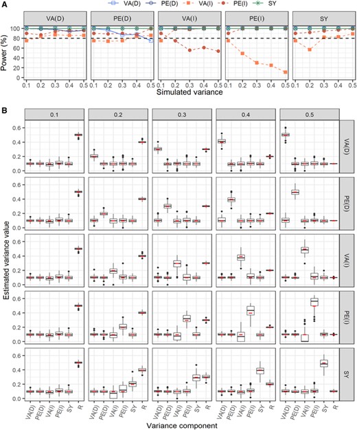
Power (A) of variance components estimated from animal models for dataset 1 (body mass, exploration, and docility) detailed in the Main text. Power of detecting significant variance components over 100 simulations is presented in each panel when one variance component (specified on top) increases in steps of 0.1 while the others are fixed to 0.1, excluding . Power significance is assumed when estimates are two times larger than their standard error. Distributions of these estimates are represented by boxplots (B) (first quartile, median, third quartile). Each horizontal panel shows the distribution of estimates of all variance components while one variance component changes in steps of 0.1 and the others are fixed to 0.1, excluding . Red lines represent the simulated values. and are respectively the direct and the indirect additive genetic variances, and are the direct and the indirect permanent environmental variance, is the season-year variance and is the residual variance.
In all simulated scenarios with dataset 1 (Fig. 3, Supporting information Figs. S1 to S3), all effects tended to have a power higher than or relatively close to 80% (>70%). The power of the indirect genetic (VAI) and environmental (VPEI) effects decreased below 80% as the variance of the other effect increased (VAI: from ∼75 to ∼10% and VPEI: from ∼90 to ∼55%). The power of VAI was always lower than the power of VPEI except when we varied VAI to values higher than 0.1.
In dataset 2 (Supporting information Figs. S4 to S7), the power of indirect effects (VAI and VPEI) varied similarly for both effects from approximately 30% to approximately 60% as the VAD, VPED, and VSY increased. When one of the indirect effect variances (VAI or VPEI) increased, the power of that effect increased and was higher than 80% for variances higher than 0.2 while the power of the other effect stabilized around approximately 20%. In all scenarios, the power of VPED was lower than the power of VAD and was lower than 80% (from ∼70 to ∼60%) when we varied VAD.
Finally, in dataset 3 (Supporting information Figs. S8 to S11), direct and indirect genetic effects had less power than in the two other datasets. However, VAD had a power higher than 80% for variances higher than 0.1 but varied from ∼30 to 90% as VAI and VSY increased (from 0.1 to 0.5). The power of VAI was stable (∼10−20%) when varying VAD, increased (from ∼10 to ∼45%) when varying VSY and was higher than 80% when its variance was higher than 0.2.
The power of the season-year effect was higher than 90% for all scenarios with all three datasets.
In simulations with dataset 1 (Fig. 3 and Supporting information Figs. S1 to S3) and 2 (Supporting information Figs. S4 to S7), the estimates of indirect effects (VAI and VPEI) were generally less accurate and precise than other components and that was more visible when we increased the variance value of one of those components.
In all scenarios, the covariances between direct and indirect effects (both genetic and permanent environmental) were poorly estimated. However, covariances had a power higher than 80% for correlation values larger than 0.6 when using dataset 1 (Supporting information Figs. S3, S7, S11).
Discussion
In this article, we addressed how social interactions contribute to variation of different types of traits through indirect genetic and permanent environmental effects in a wild chipmunk population. We implemented a novel approach (but see Fisher et al. 2019 for a first application in wild populations) that integrates the spatial structure of multiple interactions with neighbors in a quantitative genetic analysis. We found indirect genetic variance for trappability and relative fecundity, indicating that individuals’ genotypes shape the phenotypic expression of these traits in conspecifics. However, our analyses also revealed low heritability of traits and a large role for permanent environmental and social permanent environmental effects. Our study, thus, highlights how nongenetic sources of similarity between individuals (PED) and their effects on conspecifics’ phenotypes (PEI) are important in their own right, and underlines their potential adaptive value.
DIRECT AND INDIRECT GENETIC EFFECTS
Heritability estimates in our study were surprisingly low (0.01 to 0.08) and statistically nonsignificant, except for docility (Table 2; Fig. 1; see also St-Hilaire et al. 2017). Our results, thus, did not support our expectations for a higher h2 in morphological, behavioral, and physiological traits than in life-history traits (Mousseau and Roff 1987; Houle 1992; Stirling et al. 2002; Postma 2014). Furthermore, contrary to predictions (Merilä et al. 2001; Teplitsky et al. 2009; Postma 2014), we found no negative association between VAD and the covariance between the trait and fitness. The negative result may be caused by the small VAD of traits, or because the proportion of LRS explained by a trait calculated over a few years may not be representative of past selection pressures.
Traits showed little variance due to indirect genetic effects, except for trappability (0.36) and relative fecundity (0.23, marginally nonsignificant) (Table 2). Neighbors’ genotypes, thus, seem to affect the focal individual's phenotype for these two traits more than for other traits. Indirect genetic effects capture the genetic variance of “performance,” that regroups a whole set of unmeasured traits affecting a conspecific's phenotype (Moore et al. 1997; McGlothlin et al. 2010). For example, a large chipmunk may engage in more fights, which may in turn affect its neighbors growth and body mass (Santostefano et al. 2019). Further work in this area could focus on identifying which heritable traits underlie indirect genetic effects by adopting the trait-based approach (Moore et al. 1997; McGlothlin et al. 2010) which includes fitting the putative trait generating indirect genetic effects in the model. The low repeatability of fecundity (0.03) and trappability (0.21) may be caused by social effects representing more than 63 and 70% of the phenotypic variance, respectively (Table 2). In the absence of correlations between the phenotypes of focal individuals and those of their neighbors (low assortative neighboring; Santostefano et al. 2019), strong social effects can only create very strong within-individual variance and, thus, decrease repeatability and heritability.
We found no link between the magnitude of indirect genetic variance and the covariance between traits and fitness in chipmunks (Fig. 3). Indirect genetic variance in a trait may reflect direct genetic variance of traits underlying conspecific performance. For example, if body mass has small heritability, the indirect genetic variance on traits affected by conspecific body mass should also be small. Furthermore, we expect small indirect genetic effects for traits affected by performance, if traits underlying performance are highly linked to fitness and, thus, show little additive genetic variance. Further theoretical and empirical work is needed to confirm these predictions. An interesting question related to this is whether indirect genetic effects can evolve themselves. For example, maternal genetic effects occur to compensate for direct genetic effects on the phenotype and are strongest at the most important life stages (Wilson and Rèale 2006). Finding a link between selection and indirect genetic effects might give insights into the adaptive value of indirect genetic effects and be an element in favor of this hypothesis.
COMPARING CONTRIBUTIONS OF DIRECT AND INDIRECT GENETIC EFFECTS TO TRAITS EVOLVABILITY
Our results did not support the prediction for high evolvabilities of life-history traits and fitness components (Price and Schluter 1991; Houle 1992; Kruuk et al. 2000; Hansen et al. 2011). Estimates of CVa were smaller than the mean values found across studies in morphology (mean ± SE: 4.48 ± 1.46), life history (15.54 ± 1.83), behavior (13.35 ± 5.32), and physiology (10.69 ± 3.88) (Postma 2014). Overall, CVa compared to Ia, and CVige compared to Iige, provided very similar information. We also found no qualitative differences between trait types in the contribution of indirect genetic effects to evolvabilities (CVige and Iige). Thus, we found no support for the prediction that indirect genetic effects are of greater magnitude for behavioral traits, and indirect genetic effects may not provide a mechanism underlying a unique role for behavior in evolution, as suggested by Bailey et al. (2018). Because direct and indirect genetic variances in our study were mostly low and nonsignificant, we should consider our conclusions with caution. Comparing the two will be nonetheless valuable to test predictions in populations where the range of VAD and VAI is larger and therefore differences between traits detectable.
Using mean-standardized measures and comparing them to phenotypic variance-standardized measures, however, did provide insights into the evolutionary potential in response to selection of single traits. For example, sexual maturity and docility have similar point estimates for VAD, the highest in our study; however, the CVa for docility is the highest whereas it is zero for sexual maturity. This is contrary to predictions that life-history traits have low heritabilities but high evolvability, and indicates a higher evolutionary potential for a behavioral trait. In our study, traits with larger indirect genetic effects (trappability, relative fecundity) also have large CVige and Iige. Higher contribution of indirect genetic effects to evolvabilities can, thus, be due to both relative and absolute magnitude of indirect genetic effects for those traits, that is, indirect genetic effects are large also compared to other sources of variation. However, another trait (core range) with large CVige had very low (but significant) indirect genetic effects. This indicates a potential contribution of indirect genetic effects to evolvability that is masked by a larger contribution of other variance components when looking at ige2 (i.e., VAI/VP) alone. Last, we can qualitatively compare the absolute and relative importance of direct and indirect genetic effects for the evolutionary potential of a trait, by comparing within each trait the values of h2 with ige2, and CVa with CVige (or the almost equivalent Ia and Iige). Here, no clear patterns emerged, with an equal number of traits having either larger indirect genetic effects, larger direct genetic effects, or similar in magnitude.
DIRECT AND INDIRECT PERMANENT ENVIRONMENT EFFECTS
Permanent environmental effects greatly varied across types of traits, being negligible for relative fecundity, small to moderate for behaviors (0.02-0.24), and substantial for body mass (0.46; Table 2; Fig. 1). Season-year and year-of-birth effects, which we estimated separately from permanent environmental effects, also constitute sources of permanent environmental effects on individual phenotypic variation. Season-year and year-of-birth effects partly account for data censoring in life-history traits. Large permanent environmental effects can be explained by the strong ecological, behavioral, and life-history dependence of Eastern chipmunks on pulsed resources, which vary across years (Bergeron et al. 2011b; Montiglio et al. 2014; Tissier et al. 2020). When generations overlap, a highly fluctuating environment should favor the evolution of developmental plasticity instead of genetic polymorphism (Svanbäck et al. 2009). It is, therefore, not surprising to find relatively large VPED compared to the relatively negligible VAD in this chipmunk population. VPED may reflect strong developmental plasticity related to early life conditions, including nongenetic and genetic maternal effects (Kruuk and Hadfield 2007), as well as long-term effects of conditions experienced at a critical stage of life such as resource availability or population density during early development. For example, differences in population density affect parturition dates in North American red squirrels (Tamiasciurus hudsonicus) (Fisher et al. 2019). Additionally, VPED may be due to consistent differences in conditions experienced by different individuals throughout their lives (e.g., in individual territory quality and spatial distribution of resources in the environment). These effects may be generated by matching habitat choice, where phenotypically similar individuals choose similar environments (Edelaar et al. 2008). Phenotype-dependent use of microhabitats by individual chipmunks confirms those potential effects: in our study population, individual phenotypes (exploration, docility, and boldness) are nonrandomly distributed in respect to microhabitat characteristics (Gharnit et al. unpubl. ms). This distribution, however, differs depending on the grid, as the four field sites are all different and the grid is arbitrarily built in a larger patch of forest (i.e., it does not follow natural edges such as trees or rivers). Furthermore, Eastern chipmunks’ short dispersal distances (Dubuc-Messier et al. 2012) may inflate shared environmental effects, and will appear as VPED in our models. If a strong G × E correlation is present, VAD and VPED could be highly confounded and hard to interpret (Thomson et al. 2018). Furthermore, traits with large VPED relative to VAD could show strong I × E or G × E effects, as these effects are captured by VPED when they are not explicitly included in the model (Stirling et al. 2002). It is, thus, possible that part of what we estimated as VPED was caused by additive genetic effects instead.
DIRECT AND INDIRECT PERMANENT ENVIRONMENTAL EFFECTS
Indirect permanent environmental effects (VPEI) varied from negligible (0.02) for exploration, to moderate (0.39) for relative fecundity. PEI were generally larger than their genetic counterpart, as was the case for nonsocial effects (Table 2; Fig. 1). This is reasonable because we may expect the sources of VPED and VPEI to be similar. VPEI reflect effects of the social environment on the focal individual's phenotype that are not underpinned by genetic variation (see above discussion). For example, body mass variation is mostly caused by VPEI, and large neighbors decrease the fitness of chipmunks (Santostefano et al. 2019). Again, large VPEI in this population may be caused by shared environmental effects between neighbors, amplified by short dispersal distances and high relatedness between them. Thus, while indirect genetic effects only have a minor role in most of the traits considered in our study, social partners can greatly influence a trait's phenotypic expression through environmental effects. Despite this plasticity to the social environment, large VPEI compared to VAI may make a traditional evolutionary response more difficult.
Differences in magnitude of VPEI across traits may be caused by different roles played by traits in competition, as it has been proposed for indirect genetic effects (Wilson 2014), but the source of variation of these effects is nongenetic. Indeed, we found large VPEI for the two traits that also have largest indirect genetic effects, trappability, and relative fecundity. Other studies have found substantial VPEI in mammals. For example, in female North American red squirrels, timing of spring breeding, which may be a resource-limited trait, depends on the identities of their nearest neighbors (Fisher et al. 2019) whereas in domestic pigs, early-life social environment effects can in turn affect the phenotypes of social partners later in life (Canario et al. 2017). Competition over mates or food, may explain the large VPEI on fecundity or body mass, for example, an individual may monopolize mates and, therefore, impact the reproductive success and resource acquisition of its neighbors.
VPED have often been overlooked in quantitative genetics or have been only considered because they can cause upward bias estimates in VA, if not accounted for (Kruuk and Hadfield 2007). Similarly, omitting VPEI may overestimate indirect genetic effects and consequently traits heritabilities (Wilson et al. 2011; Canario et al. 2017; Kruuk and Wilson 2018). However, VPED and VPEI are an important source of nongenetic variation because they may reflect adaptive developmental plasticity. VPEI can also be interpreted as a social form of phenotypic plasticity or “social responsiveness” (Webster and Ward 2011; Taborsky and Oliveira 2012; Wolf and McNamara 2013; Wolf and Krause 2014; Dingemanse and Araya-Ajoy 2015; Santostefano et al. 2016). Plasticity may both limit evolutionary responses by shielding genotypes from selection, or facilitate evolution by generating novel phenotypes and altered selective regimes (West-Eberhard 2003; Ghalambor et al. 2007). Adaptive plasticity can also buffer effects of environmental heterogeneity (and thus strong directional selection) by allowing individuals to survive and persist in changed or novel environments (Baldwin 1896; Robinson and Dukas 1999; Ghalambor et al. 2010). Developmental plasticity could, thus, be an adaptive response to the fluctuating environmental conditions experienced by this population, which should be further tested.
VALIDITY OF THE STUDY AND ITS LIMITATIONS
The power analysis was a valuable tool to confirm that we had high power to detect indirect genetic effects at least for dataset 1 (exploration, docility, body mass) and moderate power for dataset 2 (core range area, trappability, relative fecundity), likely due to having repeated measurements per individual, whereas we should be cautious with conclusions drawn from dataset 3 (lifespan, sexual maturity). We are, thus, confident that our results support negligible indirect genetic effects for most traits. We had identifiability problems between VAI and VPEI across all datasets, as indicated by the power of detecting one effect decreasing as the variance of the other effect increased (similar as VPED being confounded with VAD, see Bourret and Garant 2017), which may also explain the large VPEI we found across traits. Our power analyses also indicate that VPEI may be overestimated, at least in dataset 1. Identifiability problems and overestimation of VPEI may, thus, partially mask VAI. In our analyses, we needed to consider the limitations of the available data, which prevented us from including maternal or common environmental effects; not explicitly modeling these effects likely increases permanent environmental effects (Kruuk and Hadfield 2007). Furthermore, not accounting for shared environmental effects between neighbors may bias heritabilities, if neighbors are clustered in time or space (Kruuk and Hadfield 2007; Thomson et al. 2018). Spatial autocorrelation also potentially contributes to the estimates of nongenetic sources of variation (Kruuk and Hadfield 2007; Regan et al. 2016), such as permanent (direct and indirect) environmental effects, if spatially close environments have similar characteristics and affect phenotypes of neighbors similarly. Implementing spatial autocorrelation in an animal model requires high power and large datasets (e.g., Stopher et al. 2012; Germain et al. 2016; Regan et al. 2016; Fisher et al. 2019, see Thomson et al. 2018 for an overview of current methods). In our case, accounting for space sharing ended up overparameterizing the models with convergence issues in all but two traits (results not shown). In the two models that did converge, spatial autocorrelation explained around 7% of the variance in body mass, and 33% in trappability. Results on these two traits suggest variance caused by spatial effects that may reduce the estimate of VPEI, which can be explained by neighbors sharing similar environments. Additionally, due to the intrinsic incompleteness of wild population data, we might have missed capturing individuals or misassigning neighbor identities, which may also have inflated VPEI.
According to our simulations, the covariances between direct and indirect effects (both genetic and permanent environmental) were poorly estimated, with high uncertainty. The requirement to phenotype, genotype, and assess the social relationships of many individuals within a population greatly limits the range of study systems where this approach can be used (Wade et al. 2010; Kruuk and Wilson 2018, e.g., see similar considerations in Fisher et al. 2019 with a larger dataset). Although we can make qualitative inferences based on the sign of correlations, our results cannot conclusively inform us on how indirect genetic effects affect the evolution of the traits considered, because we cannot reliably estimate the total breeding value (Bijma 2011), and therefore, we do not discuss them further here.
Conclusions
Our study emphasizes the role of nongenetic sources of similarity between individuals, and their effects on the expression of traits in conspecifics through a response to the social environment. This study is the first to explicitly assess the contribution of indirect genetic effects and direct genetic effects to phenotypic variation and evolvability in different trait types, a gap recently highlighted in the literature (Bailey et al. 2018). Although no clear pattern emerged, we hope this stimulates more studies to provide estimates of direct and indirect genetic effects on different types of traits to test and improve the current predictions. By relating direct and indirect genetic effects to selection strength in different types of traits, we also assessed whether genetic variability of traits assumed to be under strong directional selection (e.g., life-history traits, fitness traits), is fundamentally different from that of traits assumed to be under weak stabilizing selection (e.g., morphological traits, behavioral traits) (Merilä and Sheldon 1999). We suggest this as a fruitful area to develop new hypotheses. Finally, our study also highlighted some methodological challenges in estimating indirect genetic effects in wild populations by incorporating a simulation analysis. We emphasize the usefulness of such analyses for future studies, to assess whether the patterns uncovered are reliable. Power analyses will also help researchers to understand which structure of dataset and pedigrees is needed to answer key questions in evolutionary ecology.
AUTHOR CONTRIBUTIONS
FS and DR conceived the study. DR, DG, and PB manage the long-term chipmunk dataset.
Field assistants and undergraduate and graduate students collected the data under the supervision of DR, DG, and PB. FS and HA analyzed the data with input from DR. FS wrote the first draft of the manuscript. All authors contributed to revisions and approved the most recent version of the manuscript.
ACKNOWLEDGMENTS
We thank Nature Conservancy of Canada and Ruiter Valley Land Trust, as well as the Nature Conservancy and the Réserve Naturelle des Montagnes Vertes for access to the study sites. We are grateful to all students and research assistants who have contributed to the data collection within the Chipmunk Project since 2005. We thank David Fisher for help with statistical analyses, coding, and discussion of ideas, and Alastair Wilson for statistical advice. We thank Associate Editor Joel McGlothlin and two anonymous reviewers for feedback who greatly improved the manuscript. This work was funded by Natural Sciences and Engineering Research Council of Canada (NSERC) Discovery grants between 2005 and 2018 to DR, DG, and PB, M. Humphries, D. Kramer, F. Pelletier, and D. Thomas, and by Fonds de Recherche du Québec–Nature et technologies (FRQNT) team grants to DR, DG, PB, MH, DK and DT (2006-2009; 2011–2014; 2018–2021). FS was supported by a Deutsche Forschungsgemeinschaft individual postdoctoral fellowship, and HA by a NSERC PhD scholarship.
CONFLICT OF INTEREST
The authors declare no conflict of interest.
DATA ARCHIVING
Data is available at: https://doi.org/10.5061/dryad.000000039
LITERATURE CITED
Associate Editor: J. W. McGlothlin
Handling Editor: M. L. Zelditch
