


Abstract
Spatiotemporal variation in natural selection is expected, but difficult to estimate. Pollinator-mediated selection on floral traits provides a good system for understanding and linking variation in selection to differences in ecological context. We studied pollinator-mediated selection in five populations of Dalechampia scandens (Euphorbiaceae) in Costa Rica and Mexico. Using a nonlinear path-analytical approach, we assessed several functional components of selection, and linked variation in pollinator-mediated selection across time and space to variation in pollinator assemblages. After correcting for estimation error, we detected moderate variation in net selection on two out of four blossom traits. Both the opportunity for selection and the mean strength of selection decreased with increasing reliability of cross-pollination. Selection for pollinator attraction was consistently positive and stronger on advertisement than reward traits. Selection on traits affecting pollen transfer from the pollinator to the stigmas was strong only when cross-pollination was unreliable and there was a mismatch between pollinator and blossom size. These results illustrate how consideration of trait function and ecological context can facilitate both the detection and the causal understanding of spatiotemporal variation in natural selection.
Environmental variation in time and space is expected to generate variation in the strength and mode of natural selection (Thompson 2005; Gosden and Svensson 2008; Hereford 2009; Bell 2010; Calsbeek et al. 2012; Thompson 2013; Hendry 2017; Siepielski et al. 2017). These fluctuations may preserve genetic variation and enhance the adaptive potential of populations (Bürger 1999; Le Rouzic et al. 2013). Fluctuating selection over time and selection mosaics across space may therefore influence the resilience and persistence of biodiversity in the face of environmental change. Understanding how variation in selection affects biodiversity requires assessing the temporal and spatial scales at which selection varies (Calsbeek et al. 2012). This involves understanding the often complex links between phenotypic traits and fitness components, and overcoming uncertainties in selection estimates (Morrissey and Hadfield 2012; Morrissey 2016). The latter is important because selection is estimated with error, which must be accounted for when assessing spatiotemporal variation in selection. The challenge of distinguishing true variation in selection from sampling error is illustrated by the contradictory views provided by recent meta-analyses of temporal and spatial variation in selection (Hereford 2009; Siepielski et al. 2009, Siepielski et al. 2013; Morrissey and Hadfield 2012; Morrissey 2016; Caruso et al. 2017). Here, we argue that this problem can be mitigated by identification of ecological factors that cause variation in selection. If patterns of selection can be related to variation in ecological context, this provides additional support for the existence of biological variation in selection and, in turn, contributes to a more predictive understanding of natural selection (Arnold and Wade 1984; Wade and Kalisz 1990; Herrera et al. 2006; Calsbeek et al. 2012; Chevin et al. 2015; Siepielski et al. 2017; Gamelon et al. 2018; Clark et al. 2020).
Studies of flowering plants and their biotic interactors have yielded insights into geographic and temporal variation in phenotypic selection (Wilson 1995; Maad and Alexandersson 2004; Herrera et al. 2006; Rey et al. 2006; Gómez et al. 2009; Hereford 2009; Reynolds et al. 2010; Benitez-Vieyra et al. 2012; Benkman and Mezquida 2015; Sun et al. 2016; Emel et al. 2017). Despite their complexity, plant-animal interactions often provide tractable study systems in which both the agents of selection and the traits important for pollination success or other fitness components can be identified. For example, the opportunity for selection on floral advertisement depends on the intensities of mutualistic and antagonistic interactions (Benkman 2013; Vanhoenacker et al. 2013). Accordingly, the strength of selection on pollination traits generally increases with increasing pollen limitation (Fenster and Ritland 1994; Sletvold and Ågren 2014, 2016; Bartkowska and Johnston 2015; Trunschke et al. 2017), which may result from infrequent visitation by pollinators or inefficient pollen transfer (Harder and Aizen 2010). Pollen limitation is therefore expected to affect selection on traits influencing attraction or efficiency of pollinators. (Armbruster 1988; Solís-Montero and Vallejo-Marín 2017). Similarly, pollen limitation due to lack of pollinator service or reproductive interference from other plant species can generate selection for autonomous self-pollination (Fishman and Wyatt 1999; Moeller and Geber 2005; Opedal et al. 2016).
These arguments suggest that selection on floral phenotypes may be easier to understand by considering the ecological context in which selection is generated, such as local climate and “interactor communities” of local pollinators, antagonists, and competitors, and by making predictions about how changes in each ecological variable will influence selection on floral traits. In this respect, it is useful to distinguish among functional classes of floral traits involved in attraction (e.g., corolla size, fragrance chemistry, color patterns, quantity and quality of rewards), pollinator fit (e.g., spur length, corolla-tube dimensions, distances of rewards from anthers and stigmas), and reproductive assurance (herkogamy, dichogamy). The causes of selection may differ between functional classes, and hence the strength of selection on traits in different functional classes may covary with different ecological variables.
Pollination is one of many processes that affect plant fitness. Pollinator-mediated selection can be counteracted by selection mediated by herbivores and seed predators (Gómez et al. 2009; Pérez-Barrales et al. 2013; Vanhoenacker et al. 2013; Sun et al. 2016), and the nature and intensity of biotic interactions may depend on spatial or temporal variation in local climate or other physical factors (Thompson 2005, 2013; Campbell and Powers 2015; Hendry 2017; Siepielski et al. 2017). To estimate pollinator-mediated selection, it is therefore necessary to isolate the fitness consequences of pollination from other sources of variation in fitness. One approach is to reduce the opportunity for pollinator-mediated selection experimentally by pollen saturation and subtract the selection gradients so obtained from those obtained from open-pollinated flowers (e.g., Sletvold and Ågren 2014, 2016; Trunschke et al. 2017). An alternative approach is to isolate the process of pollen transfer statistically by defining fitness as a direct function of pollen arrival (a fitness-linked performance, see Arnold 1983), thus decoupling the fitness estimate from other (nonpollination) sources of variation (Cariveau et al. 2004; Armbruster et al. 2005; Bolstad et al. 2010; Pérez-Barrales et al. 2013).
Here, we quantify spatiotemporal variation in selection on blossom traits of the neotropical vine Dalechampia scandens. We estimate several functional components of selection using the nonlinear, path-analytical fitness-function approach developed by Bolstad et al. (2010) and Pérez-Barrales et al. (2013). To isolate pollinator-mediated selection on floral traits, we assume that the fitness component of interest is a direct function of pollen arrival. We will refer to this fitness component as “pollination fitness.” Using pollination fitness and spatiotemporal variation in selection across populations, we test (H1) if the opportunity for selection declines with increasing reliability of cross-pollination, (H2) if the mean magnitude and variance of selection gradients on traits involved in attraction and fit to the pollinators decline with increasing reliability of cross-pollination, (H3) if selection for reduced herkogamy, a trait favoring self-pollination, increases with decreasing reliability of cross-pollination, and (H4) if the strength of selection on a blossom-pollinator fit trait increases with blossom-pollinator mismatch.
Methods
STUDY SYSTEM
Dalechampia scandens L. (s.l.) (Euphorbiaceae) is a species complex of tropical vines with mixed mating systems, native to lowland Central and South America (Armbruster 1985). Plants are monoecious, but male and female flowers are aggregated into functionally integrated bisexual inflorescences, “blossoms” (Fig. 1; Webster and Webster 1972). The male subinflorescence consists of a cluster of 10 staminate flowers and a gland composed of tightly packed bractlets secreting a terpenoid resin collected by bees for nest construction, primarily female Hypanthidium (Megachilidae: Anthidiini), Euglossa, Eufriesea, and Eulaema (Apidae: Euglossini) (Armbruster 1984). The female subinflorescence consists of three pistillate flowers, each containing three ovules, resulting in a maximum of nine seeds per blossom. The male and female subinflorescences are subtended by a pair of petaloid bracts that open during the day to allow pollination and close at night. Blossoms are protogynous, with a female phase lasting two-to-three days, during which female flowers are receptive, whereas male flowers are closed. A bisexual phase of approximately six days follows, during which one-to-three male flowers elongate and open daily, whereas pistillate flowers remain receptive (Webster and Webster 1972; Armbruster and Herzig 1984; Hildesheim et al. 2019a).
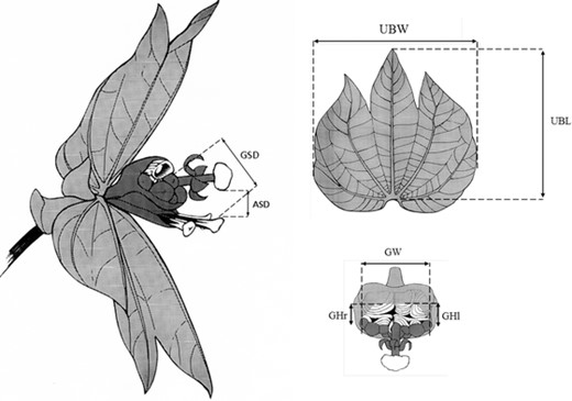
Traits measured on Dalechampia scandens blossom inflorescences. Gland-stigma distance (GSD) is the minimum distance between the resin gland and the central stigma, anther-stigma distance (ASD) is the minimum distance between the terminal male flower and the closest stigma, upper bract area (UBA) is the product of the upper bract length and width, and gland area (GA) is the product of the total gland width and the average height of the left and right gland halves. Drawings by M. Carlson.
Previous studies have identified several blossom traits of importance in pollinator attraction and pollen transfer (Fig. 1). Pollinator attraction may depend on the size of the resin-secreting surface of the gland (gland area [GA]), which reflects the amount of resin offered to the pollinator (Bolstad et al. 2010; Pélabon et al. 2012b), and on the size of the bracts (measured here as upper bract area [UBA]), which provides an honest signal of the amount of resin and functions as an advertisement to pollinators (Armbruster et al. 2005; Pélabon et al. 2012b; Pérez-Barrales et al. 2013). The fit between blossoms and visiting bees is determined by the distance between the gland and the stigmas (gland-stigma distance [GSD]), which establishes the minimum size of bees that can efficiently transfer pollen to the stigmas (Armbruster 1985, 1988; Armbruster et al. 2009b). Finally, rates of autonomous and pollinator-facilitated selfing depend on the distance between the anthers and the stigmas (anther-stigma distance [ASD]) (Armbruster 1988, 1993; Pérez-Barrales et al. 2013; Opedal et al. 2015).
DATA RECORDED
We studied phenotypic selection on the blossom traits in five populations, three in Costa Rica and two in Mexico. Both Mexican populations and one Costa Rican population were studied in two consecutive years (Table 1). The data from the La Mancha population in 2007 were from Pérez-Barrales et al. (2013). In each population, we identified distinct patches, 1-50 m apart, of one to several intertwined individuals. For the larger patches, it was sometimes difficult to distinguish individual plants, and we refer here to a patch as a collective unit of blossoms situated close to each other. The plants flower for an extended period, and we selected multiple blossoms per patch as they came into flower (median n = 4 blossoms per patch, range = 1-29).
Environmental, community, and trait characteristics of the Dalechampia scandens study populations in Costa Rica and Mexico
| La Mancha | La Mancha | Puerto Morelos | Puerto Morelos | Puente la Amistad | Palo Verde | Palo Verde | Horizontes | |
|---|---|---|---|---|---|---|---|---|
| Country (Coordinates) | Mexico N19°35′, W96°28′ | Mexico N19°35′, W96°28′ | Mexico N20°50′, W86°54′ | Mexico N20°50′, W86°54′ | Costa Rica N10°14′, W85°15′ | Costa Rica N10°23′, W85°19′ | Costa Rica N10°23′, W85°19′ | Costa Rica N10°42′, W85°35′ |
| Measurement dates | Aug 12-Sept 2, 2006 | Aug 2-31, 2007 | Sept 14-Nov 2, 2006 | Sept 15-Oct 21, 2007 | Nov 18-25, 2014 | Nov 7-15, 2014 | Oct 25-Nov 14, 2015 | Nov 15-28, 2015 |
| Sample size (# blossoms/#patches) | 135/22 | 196/33 | 211/32 | 133/26 | 99/17 | 59/20 | 132/34 | 145/39 |
| Pollinator observations | Observations (26 h) | Observations (200 h) | Observations (29 h) | Observations (21 h) | Opportunistic (∼27 h) | Opportunistic (∼24 h) | Opportunistic/ transects (∼57 h) | Opportunistic/ transects (∼42 h) |
| Pollinator genera (% observed) | Hyp. (100%) | Hyp. (72%) Eug. (28%) | Hyp. (81%) Eug. (19%) | Eug. (100%) | Euf. (61%) Eug. (26%) Hyp. (13%) | Eug. (77%) Hyp. (23%) | Euf. (50%) Eug. (31%) Hyp. (19%) | Eug. (57%) Hyp. (43%) |
| Weighted mean pollinator length (mm) | 7.00 | 8.12 | 7.76 | 11.0 | 14.7 | 10.1 | 13.7 | 9.27 |
| Proportion visited | 0.73 | 0.48 | 0.36 | 0.74 | 0.48 | 0.98 | 0.88 | 0.93 |
| Mean pollen load: female phase (SD) | 18.1 (24.9) | 11.5 (23.8) | 2.71 (9.70) | 3.24 (10.5) | 5.67 (17.6) | 25.5 (34.4) | 18.4 (23.9) | 48.8 (58.9) |
| Mean pollen load: bisexual phase (SD) | 34.1 (36.9) | 28.7 (44.3) | 5.31 (11.3) | 9.01 (14.1) | 13.4 (26.5) | 11.5 (13.9) | 11.6 (18.6) | 36.5 (49.9) |
| Mean pollen load: total (SD) | 50.9 (41.1) | 39.5 (49.0) | 7.45 (15.5) | 12.8 (18.4) | 19.0 (32.4) | 37.1 (39.2) | 29.7 (29.8) | 85.8 (72.6) |
| Mean UBA mm2 (SD) | 334 (99.0) | 488 (106) | 246 (81.6) | 264 (86.5) | 387 (106) | 495 (140) | 461 (136) | 432 (104) |
| Mean GA mm2 (SD) | 17.8 (5.69) | 13.1 (4.70) | 21.3 (7.30) | 19.8 (5.22) | 25.7 (5.69) | 29.9 (7.30) | 35.9 (8.07) | 24.0 (4.42) |
| Mean GSD mm (SD) | 4.63 (1.01) | 5.52 (0.77) | 4.84 (0.83) | 4.24 (0.81) | 4.32 (0.89) | 4.78 (0.91) | 4.94 (0.80) | 5.24 (0.95) |
| Mean ASD mm (SD) | 1.96 (1.09) | 1.22 (0.86) | 4.02 (0.96) | 4.28 (1.26) | 3.33 (1.33) | 4.91 (1.32) | 4.50 (1.11) | 2.91 (1.20) |
UBA = upper-bract area; GA = gland area; GSD = gland-stigma distance; ASD = anther-stigma distance; SD = standard deviation; Hyp = Hypanthidium; Eug = Euglossa; Euf = Eufriesea.
We followed each focal blossom throughout the female phase and for the first day of the bisexual phase. Each day, we recorded the number of pollen grains on the three stigmas with the aid of a LED light and a 10× hand lens, and whether resin had been collected. Dalechampia scandens pollen grains are large (c. 75-85 μm) and have a characteristic shape and exine, making them easy to discriminate from heterogeneric pollen. The resin is replenished daily, but its surface has an uneven texture after collection by bees. On the first day of the bisexual phase, when the first male flower was open, we counted pollen on the stigmas one last time, and we measured gland-stigma distance (GSD), anther-stigma distance (ASD), gland area (GA), and upper bract area (UBA). All distance traits were measured in millimeters using digital calipers. For the Costa Rican populations, we also measured the height of the blossom above the ground. After completing the measurements, we marked the blossoms with a small tag tied around the peduncle. We collected the marked blossoms three to four weeks later and recorded the number of seeds set (seed set). For logistical reasons, we could not collect seeds at the Puerto Morelos site.
ECOLOGICAL VARIABLES
We characterized the ecological context of pollinator-mediated selection through the reliability of cross pollination and the population-level mismatch between blossom and pollinator size.
We define cross-pollination as any pollinator-mediated pollen transfer between blossoms, including geitonogamy. We treated the mean pollen load at the end of the female phase in each population and year as a measure of cross-pollination reliability, assuming that it is inversely related to cross-pollen limitation (Opedal et al. 2016).
The methods of observing pollinator visits to blossoms varied somewhat across sites and years (Table 1). Timed observation bouts were conducted in La Mancha and Puerto Morelos when blossoms were fully open (∼1500h to 1800h). At the Costa Rican sites, we noted all pollinators observed during the collection of other data. In 2015, we supplemented these opportunistic observations with observations made along systematic pollinator transects. All bee species observed visiting blossoms were recorded. When possible, we observed whether blossom visitors contacted the stigmas. Only species observed contacting the stigmas were considered pollinators. This is a reasonable simplification, because the population mean gland-stigma distance is usually larger than the population mean gland-anther distance in D. scandens (e.g., Armbruster 1985), and, as a result, any pollinator large enough to contact stigmas will likely also have contacted anthers and carry pollen. Mean pollinator size in each population was computed by weighting the mean body length of each pollinator species, based on Michener (2000) and Roubik and Hanson (2004), by its relative proportion of visits. As an estimate of blossom-pollinator mismatch at the population level, we calculated the difference between the weighted average length of the pollinators and the average gland-stigma distance in each population and year. Note that this ignores individual variation in both blossom size and pollinator size, and is thus an incomplete measure of adaptive inaccuracy (Armbruster et al. 2004, 2009a; Pélabon et al. 2012a). Pollination efficiency is reduced when pollinators are smaller than the gland-stigma distance (Armbruster 1988, 1990), and if blossom-pollinator mismatch is the main driver of pollen limitation in the population, we might expect a correlation between pollination reliability and mismatch. We also hypothesized that pollination efficiency is reduced when pollinator size substantially exceeds gland-stigma distance. Therefore, if blossom-pollinator mismatch generates selection, we predict an increase in the strength of selection on gland-stigma distance with increasing blossom-pollinator mismatch.
PHENOTYPIC-SELECTION ANALYSIS
Levels of pollinator-mediated selection
Due to the difficulties in obtaining data on male reproductive success in natural populations (see Opedal et al. 2017), our fitness currency was based on the female reproductive success measured as the number of seeds produced by a blossom. This fitness estimate is only a component of the total fitness of the plant, and we refer to this as “pollination fitness.” Although partly imposed by the biology of a perennial plant with intertwined individuals, the choice of estimating fitness and therefore selection at the level of the single blossom also entails some advantages.
Pollinators may make foraging decisions at different levels, for example, by first choosing the plant or patch of plants to visit and then which flowers to visit on a multi-flowered plant or patch. This complicates studies of pollinator-mediated selection. We chose to focus on the average pattern of selection within patches because we were interested in the foraging decisions that generated selection on blossom traits involved in pollinator attraction, that is, traits representing advertisement (bract area) and reward (gland area). Furthermore, selection on pollination efficiency involving anther-stigma and gland-stigma distances will result from variation in the efficiency of pollen transfer within blossoms and from pollinator bodies to individual flowers, not pollinator behavior at the among-patch level.
The fitness component and the selection we infer are on the level of the individual blossom. As in any study based on fitness components, and not total fitness, the inferred selection is partial, and our measured phenotypes may be correlated with unmeasured fitness components either on the level of the blossom or on the level of the whole plant. For example, positive direct selection on blossom size may be counteracted by a negative correlation between blossom size and the number of blossoms the plant can produce. Nevertheless, by including patch as a random effect in our analysis (see below) we correct for residual correlations due to local environment and plants, and our inferences about direct selection on the blossom level should be accurate.
Selection analysis
We estimated selection gradients following Lande and Arnold (1983). Instead of analyzing observed fitness (seed set) directly, we developed a fitness function to predict the seed set for each blossom as a function of the blossom traits, that is, the number of seeds that a blossom was predicted to produce given its phenotype. This means that we first establish a set of functions describing the relationships between blossom traits and pollen load. We then obtain the predicted pollination fitness by converting the pollen load into seed set using an independently established deterministic function. The pollination-fitness function describes how phenotypic traits affect pollen deposition and incorporates functional relationships between each phenotypic trait and three sequential components: pollinator visitation, pollen load, and seed set (Fig. 2). These relationships are combined into a single predicted pollination fitness value following the methods developed by Bolstad et al. (2010) and Pérez-Barrales et al. (2013). All parameters of the path-analytical function were estimated jointly (see below). We then calculated selection gradients using the observed phenotypes and the predicted relative fitness of each blossom.
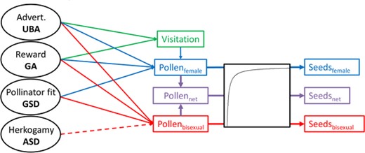
Graphical illustration of the pollination fitness function linking each D. scandens blossom trait to pollination fitness (see eqs. 1–3). The solid arrows represent hypothesized positive effects, and dashed arrows hypothesized negative effects. The number of seeds produced can increase through attraction of pollinators responding to the advertisement (UBA) or reward (GA) traits. During visitation, pollination efficiency is determined by the fit of the pollinator to the flower (GSD interacting with pollinator length). Last, pollen may be deposited onto the stigmas of the same blossom depending on the degree of herkogamy (ASD), with greater herkogamy hypothesized to reduce self-pollen load. The three pollination fitness measures, Seedsfemale, Seedsbisexual, and Seedsnet, used to estimate female-phase, bisexual-phase, and net selection are shown in blue, purple, and red, respectively.
Because pollination fitness as defined here is a direct function of pollen arrival onto stigmas, it screens off all other sources of variation in pollination-related female fitness. Pollen arriving during the female phase is deposited only by pollinators. Thus, variation in pollen load during this phase reflects variation in visitation rate and pollinator efficiency. The female-phase selection gradients obtained from the fitness function can therefore be interpreted as pollinator-mediated selection. Pollen arriving during the bisexual phase may also result from autonomous or pollinator-facilitated autogamy. Thus, the bisexual-phase and net selection gradients can be interpreted as pollination-mediated, but not necessarily as pollinator-mediated, selection.
We estimated the effects of the traits on each component of the fitness function using generalized linear mixed-effects models. For all models, patch and measurement date were included as random factors. The trait values were centered on their patch mean (), and then standardized on the population grand mean as . By centering traits on the patch means, we removed among-patch differences and fitness-trait correlations resulting from local variation in pollinator abundance and other environmental variables. Standardization by the population grand mean yields mean-scaled selection gradients that can be interpreted as the strength of selection relative to selection on fitness itself, as a trait, a useful benchmark for comparison across traits and populations (Hansen et al. 2003; Hereford et al. 2004).
STIGMATIC POLLEN LOADS
Pollen arrival during the female phase
Pollen arrival during the bisexual phase
Seed set
Because the relationship between pollen load and seed set is nonlinear, and seed set is bounded between zero and nine (Fig. 2), pollination during the bisexual phase may produce different numbers of seeds depending on the pre-existing, female-phase pollen load. The bisexual-phase selection gradients thus represent potential selection during the bisexual phase, assuming no prior pollination. In the Supporting Information, we estimate realized bisexual selection by predicting seed set resulting from bisexual-phase pollination, SB, as the difference between predicted net, S, and female-phase seed set, SF, that is, SB = S – SF (Fig. S1).
Model selection for pollination fitness components
We considered models including all blossom traits as well as all combinations of pairwise interaction terms. For parameter estimation, we retained all linear terms from equations 1–3 and used AICc (small-sample-corrected Akaike criterion) to choose which pairwise interaction terms to include in the model (Tables S1-S3). For the Costa Rican populations, we also included the height of the blossom above ground.
In a second step, we evaluated the support of the complete pollination fitness model by comparing the sum of the standard AIC (i.e., not AICc) of the component submodels (i.e., , and ), with the AIC of a model including only the intercept. This assumes that the pollination data are independent across submodels. We also computed the R2 for each component of the pollination fitness function by calculating the residual variance between the predicted and the observed value for each component of the fitness function (i.e., , and ) for each blossom, and compared this to the total variance of the pollination fitness component, , as .
Estimating strength and variation in selection
All parameters of the path-analytical fitness function were estimated jointly using the template model builder (TMB) R package (Kristensen et al. 2016), which fits nonlinear mixed-effects models with maximum likelihood. The template model builder allows estimation of derived parameters, and we obtained mean-scaled selection gradients, βnet, βfemale, and βbisexual, with standard errors by including the derived parameter, where is the phenotypic variance matrix and S is the (vector) selection differential.
To assess whether the observed variation in selection across populations and years exceeded that expected from estimation variance, we computed the spatiotemporal variance of the partial selection gradients on each trait as , where Var(β) is the observed variance of the selection-gradient estimates among populations and years, and is their average squared standard error. We subtracted the average sampling variance because variances are additive, but to express variation in selection on the same scale as the mean-scaled selection gradients, we report this as a standard deviation, , which can be interpreted as the mean dispersion of the selection estimates in units of the strength of selection on pollination fitness itself. The weighted mean of the selection gradients was calculated as , where ui is the inverse squared standard error () and n is the number of selection estimates.
Results
STRENGTH AND VARIATION IN SELECTION
The component models in the path analysis explained little variance within populations, with R2 ranging from 0% to 24% (mean: 5%, median: 3%; Table 2). Nevertheless, there was still evidence that some floral traits affected net pollination fitness in five out of the eight replicate studies (Table 2). The three exceptions were La Mancha and Puerto Morelos in 2007 and Palo Verde in 2014, where we did not detect net selection on floral traits.
Parameter estimates (± SE) from the highest ranked models for each component of the pollination fitness function. All traits were centered on the patch mean and standardized by the grand mean . Thus, the units are the change in log odds of being visited per change in trait mean or the change in log pollen per change in trait mean . The R2 is the proportion of variance explained by the model. Model selection was based on AICc, but AIC was used to obtain the summed AIC for the full pollination fitness function and is reported as (minus) the difference, ∆AIC, from the intercept-only model
| Model | Parameters | La Mancha 2006 | La Mancha 2007 | Puerto Morelos 2006 | Puerto Morelos 2007 | Puente la Amistad 2014 | Palo Verde 2014 | Palo Verde 2015 | Horizontes 2015 |
|---|---|---|---|---|---|---|---|---|---|
| Visitation | Intercept (a1), log odds | 1.28 ± 0.26 | 0.06 ± 0.19 | −0.53 ± 0.31 | 1.96 ± 0.79 | 0.01 ± 1.19 | – | 3.16 ± 1.04 | 2.69 ± 0.52 |
| 1.64 ± 1.27 | 0.79 ± 0.88 | 0.89 ± 0.79 | –0.87 ± 1.92 | 6.08 ± 2.50 | – | 4.82 ± 3.57 | 1.95 ± 2.62 | ||
| GA (b12), | 1.79 ± 0.98 | 0.13 ± 0.53 | 2.09 ± 0.77 | 0.56 ± 2.79 | –3.34 ± 2.89 | – | –0.18 ± 3.40 | –2.68 ± 3.31 | |
| Height (b13), | NA | NA | NA | NA | 8.84 ± 3.00 | – | 2.61 ± 2.12 | – | |
| UBA:GA, | – | – | – | – | – | – | –18.6 ± 11.7 | – | |
| GA:Height, | NA | NA | NA | NA | –40.1 ± 18.5 | – | – | – | |
| R2 | 4% | 1% | 11% | 0% | 12% | – | 4% | 1% | |
| # parameters | 5 | 5 | 5 | 5 | 7 | – | 7 | 5 | |
| ∆AIC | 3.4 | –2.7 | 13.0 | –3.5 | 20.9 | – | –0.2 | –2.5 | |
| Pollen (PF) | Intercept (a2), log PF | 3.06 ± 0.12 | 3.09 ± 0.19 | 1.22 ± 0.54 | 0.46 ± 0.34 | 2.02 ± 0.63 | 2.88 ± 0.23 | 2.85 ± 0.17 | 3.74 ± 0.21 |
| UBA (b21), | 1.30 ± 0.49 | 0.42 ± 1.01 | 0.60 ± 1.20 | 2.97 ± 1.21 | –4.58 ± 1.50 | 1.80 ± 1.02 | 2.17 ± 0.80 | 2.06 ± 0.84 | |
| GA (b22), | –0.47 ± 0.40 | –0.38 ± 0.66 | –0.56 ± 1.34 | –3.15 ± 1.70 | 3.00 ± 2.81 | –2.40 ± 1.07 | 0.27 ± 0.91 | 1.38 ± 0.92 | |
| GSD (b23), | –0.39 ± 0.54 | –1.27 ± 1.52 | –2.04 ± 1.86 | 5.73 ± 2.79 | –6.90 ± 2.50 | –1.50 ± 1.43 | –1.75 ± 0.95 | –0.90 ± 0.93 | |
| Height (b24), | NA | NA | NA | NA | –0.12 ± 1.88 | – | – | – | |
| UBA:GA, | – | – | 6.86 ± 3.94 | – | – | – | – | – | |
| UBA:GSD, | – | – | – | – | –22.3 ± 9.31 | – | – | –11.2 ± 4.69 | |
| UBA:Height, | NA | NA | NA | NA | 32.0 ± 8.67 | – | – | – | |
| GA:GSD, | 4.65 ± 2.37 | – | – | – | – | – | – | – | |
| GSD:Height, | NA | NA | NA | NA | 54.8 ± 16.2 | – | – | – | |
| R2 | 1% | 0% | 0% | 0% | 0 | 7% | 2% | 6% | |
| # parameters | 7 | 6 | 7 | 6 | 9 | 6 | 6 | 7 | |
| ∆AIC | 4.1 | –4.9 | –3.3 | 7.5 | 5.8 | –1.5 | 4.8 | 6.2 | |
| Pollen (PB) | Intercept (a3), log PB | 3.45 ± 0.13 | 3.31 ± 0.14 | 1.42 ± 0.3 | 1.83 ± 0.25 | 1.62 ± 0.48 | 2.42 ± 0.21 | 2.38 ± 0.24 | 3.48 ± 0.17 |
| UBA (b31), | –0.24 ± 0.54 | 0.09 ± 0.96 | 0.78 ± 0.77 | –1.14 ± 0.94 | –0.86 ± 1.03 | 0.06 ± 1.69 | 0.59 ± 1.38 | –0.41 ± 0.98 | |
| GA (b32), | –0.03 ± 0.45 | 0.55 ± 0.49 | 0.01 ± 0.75 | 4.33 ± 1.61 | –1.13 ± 1.62 | 1.79 ± 1.85 | –0.37 ± 1.96 | –0.74 ± 1.32 | |
| GSD (b33), | 0.04 ± 0.69 | –0.5 ± 1.4 | 1.37 ± 1.21 | 1.43 ± 1.99 | 6.03 ± 1.68 | 0.29 ± 1.79 | 3.01 ± 1.81 | 2.89 ± 1.30 | |
| ASD (b34), | –0.53 ± 0.29 | 0.18 ± 0.27 | –0.49 ± 1.08 | –1.18 ± 0.98 | 0.07 ± 0.55 | –1.22 ± 1.29 | 0.52 ± 1.02 | –1.07 ± 0.51 | |
| Height (b35), | NA | NA | NA | NA | – | –2.22 ± 1.71 | 1.4 ± 0.82 | – | |
| UBA:GSD, | – | – | – | – | – | – | –26.3 ± 7.31 | – | |
| UBA:Height, | NA | NA | NA | NA | – | –28.8 ± 9.83 | – | – | |
| GA:ASD, | – | –1.52 ± 0.83 | – | – | – | – | – | – | |
| GA:Height, | NA | NA | NA | NA | – | 16.8 ± 6.46 | – | – | |
| GSD:ASD, | – | – | –6.28 ± 5.87 | – | – | – | 19.7 ± 8.63 | – | |
| R2 | 1% | 0% | 9% | 14% | 3% | 6% | 24% | 20% | |
| # parameters | 7 | 8 | 8 | 7 | 7 | 10 | 10 | 7 | |
| ∆AIC | –4.9 | –5.1 | –3.8 | –3.8 | 3.3 | –2.1 | 2.1 | 2.8 | |
| SUM | ∆AIC | 2.6 | –12.7 | 5.9 | 0.2 | 30.0 | –3.6 | 6.7 | 6.5 |
UBA = upper-bract area; GA = gland area; GSD = gland-stigma distance; ASD = anther-stigma distance; ∆AIC = subtract AIC of the best ranking model from AIC of the intercept-only model; NA = height not recorded in the study.
The median magnitude of the net selection gradients in Table 3 taken over all traits, sites, and years was 11% of unit selection. This is weak when compared to the median magnitude selection gradient of 54% found in a meta-analysis of 340 multivariate selection gradients (Hereford et al. 2004). Selection varied across sites and years, but most of the spatiotemporal variation could be attributed to estimation errors in the gradients. After correcting for this, evidence for moderate spatiotemporal variation in selection remained for two of four traits (Table 3). For these two traits, gland area and gland-stigma distance, the average net selection gradients were close to zero, and their standard deviations were 13% and 17% of unit selection, respectively. In contrast, bract area, an advertisement trait, was under consistent positive directional selection across years and study sites, with an average selection gradient of 9% of unit selection. Anther-stigma distance was under negative selection at La Mancha in 2006 and at Horizontes in 2015, but overall there was no consistent evidence of directional selection on this trait.
Mean-scaled multivariate net , female-phase , and bisexual-phase selection gradients given in % (± SE), where 100% is the strength of selection on pollination fitness as a trait. The parameter is the weighed-average selection gradient, and is the standard deviation of the selection gradients across sites and years, controlled for estimation variance in the individual gradients
| La Mancha 2006 | La Mancha 2007 | Puerto Morelos 2006 | Puerto Morelos 2007 | Puente la Amistad 2014 | Palo Verde 2014 | Palo Verde 2015 | Horizontes 2015 | σβc | |||
|---|---|---|---|---|---|---|---|---|---|---|---|
| βnet | UBA | 6.15 ± 5.21 | 3.75 ± 12.0 | 57.2 ± 36.6 | 1.19 ± 29.4 | 5.28 ± 37.4 | 24.3 ± 20.2 | 29.1 ± 15.0 | 9.86 ± 6.13 | 9.41 | 0 |
| GA | 0.24 ± 4.79 | 4.87 ± 6.81 | 12.1 ± 38.3 | 94.7 ± 47.5 | 8.58 ± 62.9 | –29.9 ± 18.6 | 12.7 ± 22.2 | 4.71 ± 8.09 | 2.06 | 13.4 | |
| GSD | –1.30 ± 6.97 | –12.2 ± 17.5 | 33.5 ± 56.0 | 114 ± 69.2 | 65.9 ± 66.6 | –4.15 ± 24.2 | –13.1 ± 20.4 | 14.0 ± 9.41 | 2.57 | 17.4 | |
| ASD | –4.51 ± 2.44 | 3.14 ± 2.95 | –22.6 ± 40.9 | –35.2 ± 31.9 | 11.5 ± 15.8 | –10.3 ± 10.6 | 5.67 ± 8.25 | –5.22 ± 2.51 | –2.62 | 0 | |
| βfemale | UBA | 46.3 ± 17.1 | 32.4 ± 44.4 | 117 ± 87.6 | 221 ± 82.2 | –12.2 ± 115 | 55.2 ± 32.9 | 71.7 ± 26.7 | 35.8 ± 16.2 | 48.9 | 32.2 |
| GA | 3.51 ± 15.0 | –13.0 ± 29.0 | 76.2 ± 99.9 | –243 ± 104 | 164 ± 136 | –73.0 ± 33.5 | 17.4 ± 32.3 | 33.2 ± 17.7 | 4.75 | 93.2 | |
| GSD | –8.22 ± 17.2 | –51.0 ± 61.1 | –113 ± 127 | 366 ± 141 | –227 ± 123 | –48.0 ± 46.5 | –65.6 ± 31.9 | –8.44 ± 20.1 | –19.6 | 148 | |
| βbisexual | UBA | –5.50 ± 11.4 | –1.27 ± 20.9 | 50.2 ± 49.6 | –55.9 ± 47.9 | –37.2 ± 47.7 | –26.6 ± 57.4 | 1.14 ± 52.7 | –11.4 ± 21.0 | –6.98 | 0 |
| GA | –0.27 ± 8.92 | 14.4 ± 11.2 | –1.71 ± 48.5 | 207 ± 66.4 | –61.0 ± 85.9 | 13.5 ± 56.4 | 20.3 ± 79.3 | –10.2 ± 25.8 | 6.08 | 56.2 | |
| GSD | 1.18 ± 14.2 | –9.98 ± 31.0 | 92.6 ± 75.2 | 70.6 ± 96.6 | 306 ± 84.9 | 87.6 ± 72.1 | 25.0 ± 61.8 | 60.6 ± 30.3 | 18.9 | 75.4 | |
| ASD | –10.5 ± 5.98 | 7.18 ± 5.89 | –38.3 ± 65.6 | –59.1 ± 48.7 | 4.45 ± 29.0 | –37.6 ± 51.2 | 7.96 ± 39.5 | –18.2 ± 9.81 | –4.49 | 0 |
Decomposing selection into female- and bisexual-phase components revealed a different picture, with much stronger and more variable selection within each phase. The average magnitude of selection gradients for the female and bisexual phases were 88% and 42% of unit selection, respectively, compared to 21% for net selection. Part of the variation across time and space was again due to estimation error, but substantial variation remained in female-phase selection after correcting for estimation error (Table 3). For gland-stigma distance, directional selection tended to change sign between the female and bisexual phases with average selection gradients of −20% and 19% of unit selection in the female and bisexual phases, respectively (Fig. 4; Table 3).
ECOLOGICAL CONTEXT AND SELECTION
Cross-pollination reliability as measured by the mean female-phase pollen load varied across populations from 3.2 pollen grains per blossom at Puerto Morelos in 2006 to 48.8 pollen grains per blossom at Horizontes in 2015, whereas variation across years was more limited. This range translates into considerable variation in predicted seed set. The shape parameter of the diminishing-return function that translates the number of pollen grains into number of seeds (eq. 4) was estimated at α = 0.138 odds of producing a seed per pollen grain. Because the maximum number of seeds is nine, this translates 5 pollen grains into 3.67 seeds, and 50 pollen grains into 7.86 seeds.
The spatiotemporal variation in pollination reliability was related to the strength and opportunity for selection. As expected from hypothesis H1, the opportunity for pollinator-mediated selection during the female phase declined with increasing cross-pollination reliability (Fig. 3A). Furthermore, both the mean magnitude and variation in selection during the female phase decreased with increasing cross-pollination reliability, as predicted from hypothesis H2 (Fig. 3B). We observed a similar pattern for selection during the bisexual phase and for net selection on those traits for which selection varied (Figs. 3C-F). In contrast, we found no evidence for hypothesis H3; selection on anther-stigma distance, which affects self-pollination, was not clearly related to the reliability of cross pollination.
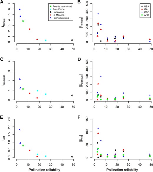
Population-level effects of cross-pollination reliability, measured as average pollinator-mediated pollen load, on the predicted opportunity for selection and on the magnitude of selection gradients . Opportunity for selection is the variance in relative pollination fitness (relative number of seeds). The mean-standardized selection gradients are given in %, where 100% is the strength of selection on pollination fitness as a trait.
The diversity and composition of pollinator assemblages varied across years and populations, with the number of visiting pollinator species ranging from one (either Euglossa cf. dilemma or Hypanthidium cf. melanopterum) to three (E. cf. dilemma, H. cf. melanopterum, and Eufriesea sp.; Table 1). This generated differences in average pollinator lengths among study sites, with a maximum difference of 7.7 mm between La Mancha 2006 and Puente la Amistad 2014, and between years within study sites ranging from 1.1 mm at La Mancha to 3.6 mm at Palo Verde. Blossom-pollinator mismatch ranged from pollinators being 2.6 to 10.4 mm longer than the average gland-stigma distance (Table 1). Given these differences, we expected to see a positive relationship between mismatch and the strength of selection on gland-stigma distance (hypothesis H4). Net selection on gland-stigma distance to decrease mismatch tended to be stronger when substantial mismatch occurred in combination with low pollination reliability, as at Puerto Morelos in 2006 and Puente la Amistad in 2014 (Fig. 4B). This result held also for realized bisexual-phase selection (Fig. S3), and the combined effect indicates that blossom-pollinator mismatch is unlikely to be the main driver of pollination reliability. This is further supported by our failure to detect consistent negative correlations between mismatch and pollen arrival onto stigmas during either the female phase (correlation = –0.15, 95% CI = (−0.77, 0.62); Fig. 4A) or the bisexual phase (correlation = −0.46, 95% CI = (−0.88, 0.36); Fig. 4A).
![Population-level relationships between blossom-pollinator mismatch (quantified as the difference between the average gland-stigma distance [mm] and the weighted average pollinator length [mm]) and (A) net (black squares), bisexual-phase (blue circle), and female-phase pollen loads (red triangles), and (B) selection on gland-stigma distance. The mean-standardized selection gradients are given in %, where 100% is the strength of selection on pollination fitness as a trait. The dotted line indicates no selection and each point represents a population estimate. Error bars indicate ± one standard error.](https://oup.silverchair-cdn.com/oup/backfile/Content_public/Journal/evolut/75/2/10.1111_evo.14136/2/m_evo14136-fig-0004.jpeg?Expires=1747932528&Signature=JaWEBTcKZ5GAPyPcYHe-TvQP92yoTU~Ng2DEln5cDjcGgF445LY4o8hO41zValTQrkDJ79eDn4TNu-1uB9f1QYhRCyJCucNy55JgeJonHybBGwqhs5C1B2Q3SjgpcBQ1iBRv~XDpYJowY1YdwFE3wUMJ5V8KbzWV8uoCKFJApGO47~revYNzXI-FrYnUclgKC6MxVS-EQ-ZaVfIQKr7l9A1p-I8dFZ--DxIIJdDEA8riFWA0lrna9QJhPcPVSkHTPD988T8z5i4Bb4Xu6lmb7~IYC~h7p-4VQcFVpiB9oKN33rbxry2Xiw47x0yxAu~~f8yebmA97wpwslN9etHmFg__&Key-Pair-Id=APKAIE5G5CRDK6RD3PGA)
Population-level relationships between blossom-pollinator mismatch (quantified as the difference between the average gland-stigma distance [mm] and the weighted average pollinator length [mm]) and (A) net (black squares), bisexual-phase (blue circle), and female-phase pollen loads (red triangles), and (B) selection on gland-stigma distance. The mean-standardized selection gradients are given in %, where 100% is the strength of selection on pollination fitness as a trait. The dotted line indicates no selection and each point represents a population estimate. Error bars indicate ± one standard error.
Discussion
Geographical and temporal variation in natural selection is expected to be common, but is difficult to detect due to the uncertainty associated with estimates of selection (Herrera et al. 2006; Bell 2010; Calsbeek 2012; Calsbeek et al. 2012; Morrissey and Hadfield 2012; Siepielski et al. 2013, Chevin et al. 2015; Morrissey 2016; Siepielski et al. 2017). We argue here that the reliability of selection estimates can be assessed and improved by considering how selection covaries with local ecological factors likely to affect fitness and trait-fitness relationships. In the present study, we were able to link variation in pollinator-mediated selection to variation in ecological context across time and space, and by decomposing the selection into ecological components, we were able to estimate and test hypotheses about subcomponents of selection, even when they balanced out so that the net selection was too weak to be statistically detectable.
The opportunity for pollinator-mediated selection is expected to increase with decreasing rates (reliability) of pollination, because average seed set will increase at a diminishing rate with the number of pollen grains deposited onto stigmas. When all ovules are fertilized, there is no more room for variation in female fitness, at least in terms of seed quantity, and, consequently, no opportunity for pollinator-mediated selection through seed number. Thus, if specific floral traits affect pollinator attraction or the efficiency of pollen transfer, low rates of cross-pollination will be associated with greater opportunity for selection (Vanhoenacker et al. 2013). Our results are largely consistent with these expectations, because both the opportunity for selection and the average strength of pollinator-mediated selection decreased with increasing reliability of cross-pollination at the population level.
Most studies demonstrating relationships between pollen limitation and the strength of pollinator-mediated selection are based on cross-species comparisons (Sletvold and Ågren 2014; Bartkowska and Johnston 2015; Trunschke et al. 2017). Except under experimental conditions (Sletvold and Ågren 2016; Panique and Caruso 2020), studies comparing conspecific populations have rarely detected the expected patterns, possibly due to limited variation in pollen limitation among populations (Sletvold and Ågren 2014; Bartkowska and Johnston 2015). Our study is the first to examine pollinator-mediated selection across a large natural gradient in cross-pollination reliability within a species. This large range of cross-pollination reliability also increases variation in seed production among populations and, thus, our ability to detect a relationship between cross-pollination reliability and strength of selection.
We also observed increased variation in selection strength when cross-pollination reliability was low. Similar patterns have been observed in orchids (Sletvold and Ågren 2014; Trunschke et al. 2017) and in comparisons across more disparate taxa (Ashman et al. 2004; Bartkowska and Johnston 2015), suggesting a general relationship between ecological context and variation in selection on floral traits. Specifically, selection is always weak when pollination reliability is high, whereas selection at low pollination reliability may or may not be strong, depending on factors such as variation in the functional relationships between traits and fitness (Sletvold and Ågren 2014). Indeed, low cross-pollination reliability, as captured by low conspecific pollen loads on stigmas at the end of the female phase, integrates two semi-independent processes, pollinator-visitation rate and pollination efficiency (e.g., Armbruster 1988).
Unsurprisingly, we found that variation in pollination reliability influenced variation in selection on traits related to attraction and efficiency of pollinators. To disentangle these effects, we further assessed the role of fit to the pollinator by relating selection to variation in blossom-pollinator mismatch. As expected, we detected net selection in populations with low rates of pollination and poor match between pollinator size and blossom morphology; for example, at Puente la Amistad in 2014 and Puerto Morelos in 2007. Interestingly, at Puente la Amistad positive net selection on gland-stigma distance was driven primarily by positive selection during the bisexual phase, whereas at Puerto Morelos it was driven by positive selection during the female phase. We can only speculate about the causes of this difference, but field observations suggest that the pollinator species differed in their relative preference for bisexual blossoms. In particular, 86% of the foraging bouts of Eufriesea, the largest pollinator, were initiated on bisexual blossoms, which could explain the positive bisexual-phase selection for larger gland-stigma distances in the Eufriesea-pollinated Puente la Amistad population. Indeed, open male flowers of D. scandens are comparatively showy, relative to other blossom parts, with ample pollen of a pale yellow hue, a color known to elicit landing responses in pollinators as diverse as bumblebees and syrphid flies (Lunau 1991, 1992, 2000). Differences in selection to match pollinators have also been documented in other systems in which pollinator identity varies over time or space (Sahli and Conner 2011; Kulbaba and Worley 2013; Campbell and Powers 2015; Chapurlat et al. 2015). More data on how selection to fit the size, shape, and behavior of pollinators relates to the composition of the pollinator community are needed both for understanding pollinator-mediated selection and for predicting the consequences of local extinctions in pollinator communities (Opedal 2019).
Lack of pollinator service can also generate selection for autonomous self-pollination (Fishman and Wyatt 1999; Moeller and Geber 2005; Opedal et al. 2016), and therefore we expect negative selection on anther-stigma distance when cross-pollination is unreliable. Given that autonomous selfing is more likely to occur during the end of the bisexual phase, our focus on pollen arrival during the early bisexual phase may be the reason we were unable to detect the expected pattern.
The arguments above assume that seed quality is independent of pollen quality, but this is unlikely to be the case (Aizen and Harder 2007; Harder et al. 2016). In D. scandens, seed size tends to increase at larger pollen loads, suggesting an effect of sampling from pollen grains of unequal quality (Hildesheim et al. 2019b). Thus, the common use of seed number as a proxy for female fitness may underestimate the strength of selection for pollinator attraction and efficiency. Variation in post-pollination selection of pollen may further add to spatiotemporal variation in natural selection.
The causal basis of selection on flowers can be studied experimentally with trait manipulation (e.g., Armbruster et al. 2005), pollinator exclusion (Fishman and Willis 2008), or supplemental pollination (e.g., Caruso et al. 2019). As an alternative to experimental manipulations, one can also test causal hypotheses by studying how selection gradients change with environmental variables (Wade and Kalisz 1990). A variety of methodological tools to conduct such analyses are now available, including path-analytical approaches (Schemske and Horvitz 1988; Crespi and Bookstein 1989; Mitchell-Olds and Bergelson 1990; Mitchell 1994; Scheiner et al. 2000; Morrissey 2014) and other methods that partition selection among hierarchical levels or functional components (Heisler and Damuth 1987; Armbruster 1988, 1991; Arnold 2003; Ridenhour 2005; Walker 2007; see also Chenoweth et al. 2012; Frank 2013). In our study, we have used the nonlinear causal fitness-modelling approach developed by Bolstad et al. (2010) and Pérez-Barrales et al. (2013). This approach allowed us to integrate knowledge of trait function with observational data to understand how the strength and mode of selection varied across sites and years. Compared with experimental approaches, this approach is more flexible in combining quantitative results across selection events, which may be difficult in face of the context specificity of experimental results. See also Shaw and Geyer (2010) and Morrissey and Sakrejda (2013) for related approaches.
A predictive understanding of adaptive evolution requires the identification of general factors associated with variation in the strength and mode of natural selection. For example, a recent global-scale meta-analysis found that variation in precipitation explained a substantial proportion of variation in selection gradients (Siepielski et al. 2017). Regarding selection on floral traits, effects of climate may often be mediated by variation in the communities of interacting species. For example, if a pollinator responds to variation in climate, an effect of climate on selection might appear. Our study of selection on D. scandens blossoms has revealed temporal and spatial variation in selection that can be partly explained by ecological variation in biotic interactions. These results support the hypothesis that cross-pollen limitation is a key modifier of selection on floral traits at the level of the blossom. They further suggest that spatiotemporal variation in pollinator-assemblage composition, as well as pollinator abundance, may drive variation in pollen limitation and pollinator-mediated selection on floral traits. This demonstrates that explicit consideration of ecological and functional contexts can facilitate identification of the causes of variation in natural selection.
AUTHOR CONTRIBUTIONS
The project was initiated by CP, WSA, TFH, ØHO, and EA. RPB handled research permits. RPB, EA, ØHO, GHB, and WSA collected field data. EA analyzed data with contributions from GHB. EA, ØHO, and CP led the writing, and all authors contributed to revisions.
ACKNOWLEDGMENTS
We thank MINAE and SINAC for permission to work in protected areas in Costa Rica, the staff of OTS Palo Verde and Estación Horizontes for their hospitality and assistance, and M. Blanco for logistical support. We also thank J. López-Portillo and J. García Franco from INECOL and ECOSUR for providing access to Centro de Investigaciones Costeras “La Mancha” and to Jardín Botánico Dr. Alfredo Barrera Marín, respectively, in Mexico. We further thank P. Hanson for identifying euglossine bees and A. Sandria, J. Bush, J. Moss, F. Ashwood, E. Bengtsson, and J. Fierst for field assistance. This study was supported by the Research Council of Norway through its Centers of Excellence funding scheme, project no. 223257, and via project 287214 to CP. Fieldwork in Costa Rica by ØHO, WSA, and RPB was supported by the Royal Norwegian Society of Sciences and Letters, The Royal Society (UK), and The British Council, respectively. Fieldwork in Mexico by RPB and WSA was supported by National Science Foundation (USA) grant no. DEB-044745 to WSA. CP and TFH were hosted at the Center of Advanced Study (CAS) in Oslo during the writing of this article.
DATA ARCHIVING
Data are accessible from Dryad: https://doi.org/10.5061/dryad.0k6djh9xx.
LITERATURE CITED
Associate Editor: S. Glemin
Handling Editor: D. Hall
