


Abstract
Detection of footprints of historical natural selection on quantitative traits in cross-sectional data sets is challenging, especially when the number of populations to be compared is small and the populations are subject to strong random genetic drift. We extend a recent Bayesian multivariate approach to differentiate between selective and neutral causes of population differentiation by the inclusion of habitat information. The extended framework allows one to test for signals of selection in two ways: by comparing the patterns of population differentiation in quantitative traits and in neutral loci, and by comparing the similarity of habitats and phenotypes. We illustrate the framework using data on variation of eight morphological and behavioral traits among four populations of nine-spined sticklebacks (Pungitius pungitius). In spite of the strong signal of genetic drift in the study system (average FST = 0.35 in neutral markers), strong footprints of adaptive population differentiation were uncovered both in morphological and behavioral traits. The results give quantitative support for earlier qualitative assessments, which have attributed the observed differentiation to adaptive divergence in response to differing ecological conditions in pond and marine habitats.
The study of ultimate and proximate determinants of population differentiation in traits of ecological importance—both in spatial and temporal contexts—is central to contemporary evolutionary biology research. Attempts to identify, understand, and infer selection pressures responsible for local adaptation in various taxa are vigorous areas of research (Kawecki and Ebert 2004; Leinonen et al. 2008; Hereford 2009; Nosil et al. 2009; Blanquart et al. 2012). Similarly, much research and debate has been centering around reconciling whether observed phenotypic changes in mean values of phenotypic traits over time represent evolutionary responses to natural selection, or merely plastic phenotypic responses to changing environmental conditions (Gienapp et al. 2008; Kuparinen and Merilä 2008; Pujol et al. 2008; Brommer 2011).
Apart from the problem of differentiating between genetic and environmental causes of population differentiation, evolutionary studies are also faced with the problem of distinguishing between adaptive and “neutral” explanations for observed divergence. Although methods for inferring action of natural selection at the molecular level keep on developing and have found many uses in evolutionary biology (Egea et al. 2008; Foll and Gaggiotti 2008; Coop et al. 2010; Brommer 2011; Narum and Hess 2011), their utility is limited in the sense that they normally cannot be used to detect selection on quantitative traits. One of the main reasons for this is the highly polygenic basis of quantitative traits, and the fact that the magnitude of differentiation at individual coding loci is not expected to differ much from that of the neutral loci (McKay and Latta 2002; Le Corré and Kremer 2012). To this end, QST − FST comparisons (e.g., Merilä and Crnokrak 2001; Whitlock and Guillaume 2009; Leinonen et al. 2013) have provided a practical way to infer action of natural selection on quantitative traits. In brief, if QST, an index of divergence in quantitative traits (Spitze 1993), exceeds FST, a measure of random genetic drift estimable from neutral molecular markers (Rousset 2002), there is evidence for the action of diversifying natural selection.
Although judicious application of the QST − FST comparisons can provide a good platform to detect signatures of natural selection (e.g., Rhone et al. 2010; Leinonen et al. 2013), the method has various limitations. Among other things, its standard implementation requires a fairly large number of populations to be compared in order to have a reasonable statistical power to pick up signatures of selection (O'Hara and Merilä 2005; Ovaskainen et al. 2011). Another issue is that the method's power to discriminate between natural selection and random genetic drift is compromised when the baseline level of “neutral” differentiation, that is FST, becomes high (Hendry 2002). Both of these shortcomings are circumvented by the method of Ovaskainen et al. (2011), which has been as yet little used because of its computational complexity and lack of ready-to-use scripts to implement it—a situation which has recently changed (Karhunen et al. 2013). Nevertheless, the method has been only applied to one case study so far (Karhunen et al. 2013), and even then, merely for illustrative purposes.
Both QST − FST comparisons and the method of Ovaskainen et al. (2011) ignore habitat information and focus only on demographic processes, and in the case of the latter, on genetic correlations among traits (Ovaskainen et al. 2011). However, given that random processes such as genetic drift are not expected to result in independent evolution of similar phenotypes in different localities (e.g., Schluter 2000; Langerhans and DeWitt 2004), also habitat information is likely to carry useful information about causes of population differentiation. Hence, the analytical framework of Ovaskainen et al. (2011) could be improved by developing it to account for habitat information and its correlation with observed phenotypes. In other words, it should—at least sometimes—be possible to enhance the power to detect the footprints of selection in the framework of Ovaskainen et al. (2011) by developing a new statistical test which would incorporate data on environmental variables.
Pond populations of the nine-spined stickleback (Pungitius pungitius) provide an interesting and challenging case—both biologically and methodologically—to detect footprints of natural selection in the past. They have evolved similar morphological (Herczeg et al. 2009a, 2010; Ab Ghani et al. 2012; Välimäki et al. 2012), life history (Herczeg et al. 2012; Ab Ghani et al. 2013), behavioral (Herczeg et al. 2009b,2009c, 2013; Herczeg and Välimäki 2011; Ab Ghani et al. 2012), neuroanatomical (Gonda et al. 2009a,2009b, 2012; Trokovic et al. 2011, 2012), and physiological (Waser et al. 2010) phenotypes independently in different Fennoscandian localities. Common-garden experiments have shown that the observed differentiation has a genetic basis for many of the studied traits (Ab Ghani et al. 2012, 2013; Herczeg et al. 2012). At the same time, the pond populations are subject to severely reduced neutral genetic variability and strong genetic drift (Shikano et al. 2010; Bruneaux et al. 2013) which poses challenges for detecting signals of natural selection by QST − FST type of methods (Hendry 2002). Therefore, standard QST − FST comparisons are unlikely to work here (but see Shimada et al. 2011 for a contrary example), or at least, they are expected to have a very low statistical power to do so. Similar problems will be faced in many other contexts too, and a good case in point is provided by the contrast between freshwater and marine fishes in general: due to their restricted gene flow and smaller effective population sizes, freshwater fish show much more population structuring in neutral marker genes than marine fish (Ward et al. 1994; DeWoody and Avise 2000; DeFaveri et al. 2012). Hence, as indicated by recent theoretical treatments (Kronholm et al. 2010; Le Corré and Kremer 2012), QST − FST comparisons are unlikely to be of much help in distinguishing neutral and selective differentiation in these systems.
The main aims of this study were twofold. First, to extend the method of Ovaskainen et al. (2011) to detect footprints of natural selection in quantitative traits by introducing a new statistical test (H test) to infer whether populations found in similar habitats are more similar to each other than expected by chance, that is on the basis of their shared evolutionary history and genetic correlations among traits. Unlike the hierarchical QST − FST comparisons (Chapuis et al. 2008; Whitlock and Gilbert 2012), the method developed here does not require the habitats to fall in discrete classes or types. Instead, they may be described through a set of both continuous and categorical variables. Second, using this extended analytical framework, we looked for signatures of habitat-specific diversifying selection in five morphometric and three behavioral traits in nine-spined sticklebacks. To this end, we are able to provide the first formal demonstration of natural selection (but see Shimada et al. 2011) in this extensively studied model system, where earlier studies have provided only indirect indications for adaptive differentiation in a range of quantitative traits (reviewed by Merilä 2013).
Methods
STUDY SPECIES AND POPULATIONS
The nine-spined stickleback is distantly related to its better-known congener—the three-spined stickleback (Gasterosteus aculeatus)—but differs from it by being more widely distributed in freshwater habitats (Wootton 1984). It also shows much more genetic structuring in neutral marker genes over comparable ranges both in freshwater and marine habitats than the three-spined stickleback (DeFaveri et al. 2012). In spite of being subject to strong random genetic drift, studies of Fennoscandian freshwater populations of the nine-spined stickleback have uncovered evidence for widespread environmental adaptation (Merilä 2013).
The populations included into this study comprise of two sea (Helsinki, Baltic Sea, 60°13′N; 25°11′E and Levin Navolok Bay, White Sea, 66°18′N; 33°25′E) and two pond (Åmsele, Bynästjärnen, 64°27′N; 19°26′E and Kuusamo, Pyöreälampi 66°15′N; 29°26′E) populations (Fig. 1). These populations were chosen to represent two independent postglacial colonizations of freshwater habitats from two different ancestral marine populations (Shikano et al. 2010; Bruneaux et al. 2013).
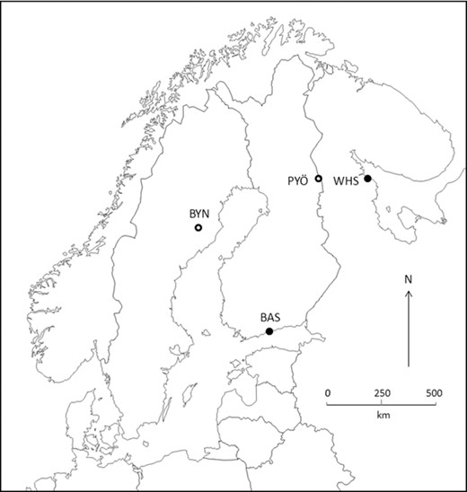
Map showing the location of study sites. The fish used as the parental generation in the common-garden study originate from the following populations: BAS = Baltic Sea, WHS = White Sea, PYÖ = Pyöreälampi, and BYN = Bynästjärnen. BYN and PYÖ represent independent postglacial colonizations from BAS and WHS, respectively. Closed dots denote marine habitats and open dots denote ponds.
THE DATA
A total of 92 F1-generation fish born to wild-collected parents were reared in a common-garden environment in the aquaculture facilities of the University of Helsinki from June–July 2007 to March–April 2008. These data have earlier been used for instance by Herczeg et al. (2009a,2009b; 2012), and the detailed rearing procedures have been described in these publications: For each population, five full-sib families were produced using wild-caught parental fish, that is five independent parental fish of each sex from each population. The offspring were reared from hatching until the age of 256 days, of which 92 individuals (Baltic Sea = 21; White Sea = 24; Bynastjärnen = 22; Pyöreälampi = 25) were chosen at random to be used in this study, whereas the rest were used in neuroanatomical studies (Gonda et al. 2009a). At the end of the experiment, the fish were killed with an overdose of tricaine methanosulphonate, digital photographs were taken from the left side of each fish, and five morphological traits were measured from the photographs, using landmark coordinates and basic Euclidean geometry. For the description of landmarks, see Figure 2 in Herczeg et al. (2010). The five morphological traits included in this study are: standard length (distance between landmarks 1 and 8; a proxy of body size), body depth (distance between landmarks 4 and 12), head length (distance between landmarks 1 and 13), pelvic girdle length (distance between landmarks “X” and 4), and caudal peduncle length (distance between landmarks 6 and 7. All measurements were taken with programs tpsDig 2 (Rohlf 2008) and tpsRelw 1.46 (Rohlf 2007).
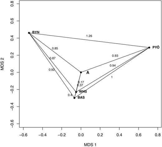
The pattern of genetic differentiation inferred from neutral genetic markers. The local populations were mapped into a 2D coordinate system by using multidimensional scaling. The numbers marked along the lines indicate genetic distances between the populations, measured in units of ancestral SD of a neutral trait (see Karhunen et al. 2013 and main text). The pattern of phenotypic differentiation is expected to be similar under random genetic drift. The figure has been produced by modifying the code of viz.theta in driftsel (Karhunen et al. 2013). “A” refers to the unobserved ancestral population.
The three behavioral traits, taken from same individuals and earlier analyzed by Herczeg et al. (2009b), were the following: number of attacks against a stimulus conspecific (henceforth: “aggressiveness”), time till the fish fully came out from a refuge in a new, potentially dangerous situation (henceforth: “risk taking 1”), and time till the first biting attempt on familiar food after a simulated attack (henceforth: “risk taking 2”). However, the distribution of “risk taking 2” was found to be highly skewed, with almost half of the fish not biting at all during the 300-s-long trials, and most of the rest biting during the first few seconds. Thus, we coded “risk taking 2” as a binary variable such that value 1 was assigned for the fish that tried to bite in <300 s, and value 0 was used otherwise. The raw data are summarized in Table 1.
Summary of raw data. Reported are the mean (± SE) phenotypic values in the offspring (F1) generation of the common-garden study. Feeding denotes the binary decision to feed or not during a 300 sec experimental time; thus, the population means of feeding can to be interpreted as probabilities. The right-hand columns (R2) show the proportion of phenotypic variation explainable by habitat and population, respectively. These were obtained from a conventional ANOVA model with sex, habitat, and population (nested within habitat) as explanatory variables. n = number of individuals
| Baltic Sea | White Sea | Bynästjärnen | Pyöreälampi | R2 of | R2 of | |
| Trait | (n = 21) | (n = 24) | (n = 22) | (n = 25) | habitat (%) | population (%) |
| Morphology | ||||||
| Standard length (mm) | 46.5 (±1.0) | 60.4 (±0.8) | 68.7 (±0.8) | 72.1 (±1.3) | 50 | 31 |
| Body depth (mm) | 8.7 (±0.2) | 10.8 (±0.2) | 12.9 (±0.1) | 13.0 (±0.2) | 57 | 26 |
| Head length (mm) | 10.1 (±0.1) | 12.0 (±0.1) | 14.1 (±0.1) | 15.7 (±0.1) | 39 | 53 |
| Pelvic girdle length (mm) | 6.7 (±0.2) | 8.2 (±0.1) | 6.8 (±0.2) | 8.3 (±0.2) | 0 | 39 |
| Caudal peduncle length (mm) | 7.0 (±0.3) | 10.3 (±0.3) | 10.6 (±0.2) | 10.1 (±0.4) | 36 | 11 |
| Behavior | ||||||
| Aggression (number) | 4.6 (±2.0) | 4.0 (±1.6) | 9.1 (±1.7) | 15.6 (±2.0) | 3 | 24 |
| Risk taking 1 (sec) | 273 (±61) | 438 (±49) | 115 (±30) | 119 (±31) | 5 | 29 |
| Risk taking 2 (binary) | 0.22 (±0.10) | 0.23 (±0.09) | 0.74 (±0.11) | 0.86 (±0.08) | 12 | 22 |
We note that although driftsel analyses—including the new H test introduced later—can be in principle performed using wild-collected (i.e., purely phenotypic) data (Karhunen et al. 2013, p. 747), results of such analyses should be interpreted with caution as they do not differentiate between environmental and genetic influences on phenotypes. However, as our analyses are based on common garden reared fish, we assume that our estimates of population differentiation are reflective of genetic differences among populations.
To obtain estimates of neutral genetic differentiation, the genetic variability of 12 unlinked microsatellite markers was assessed using the R package RAFM (Karhunen and Ovaskainen 2012). These data derive from Shikano et al. (2010), and comprise the genotypes of 183 individuals (Baltic Sea = 40, White Sea = 40, Bynastjärnen = 40, Pyöreälampi = 63) in the following loci: 1125P, 4174P, 7033P, Stn49, Stn96, Stn100, Stn130, Stn163, Stn173, Stn196, Stn198, and Stn380. Data on genetic variability and full characterization of microsatellite marker data can be found from Shikano et al. (2010). All these data have been uploaded to Dryad doi: 10.5061/dryad.sg546.
STATISTICAL METHODS
We analyzed the data with the R package driftsel (Karhunen et al. 2013), which we extend in this study to accommodate binary traits (see Appendix A and Fig. A1) and habitat information. The updated version of driftsel that implements the new statistical test is available at http://www.helsinki.fi/biosci/egru/software/. The new version has been also uploaded to CRAN (http://cran.r-project.org/).
driftsel delivers the joint posterior distribution for a number of parameters, including the mean additive genotypes of the local populations (“population means”), the unobserved ancestral means, and the ancestral G matrix. Their joint distribution can then be postprocessed in driftsel to calculate the signal of selection S (Ovaskainen et al. 2011). This figure is interpreted such that implies perfect match with random genetic drift, whereas implies stabilizing natural selection at a 95% credibility level, and implies divergent natural selection at this credibility level. This statistic takes into account the pattern of relatedness among local populations as well as the ancestral genetic correlations, but does not use habitat information. Therefore, we develop here a new test statistic H which has a similar interpretation as S, but takes into account also the correlation between genotypes and habitats. In a nutshell, the test statistic H measures the similarity between the distribution of quantitative traits and the distribution of environmental conditions, taking into account the fact that populations found in similar habitats may have a shared phylogenetic history. We will explain the derivation of H later.
In this particular case of the nine-spined stickleback, we use a single categorical variable to describe the habitats, that is we label the habitats as either pond or marine, but the developed method can use an arbitrary number of both discrete and continuous environmental variables. However, it should be noted that once the number of environmental variables to be analyzed increases, typical problems associated with multiple testing arise. Thus, the method will require larger number of populations to have sufficient statistical power to pick up similarity between the distribution of quantitative traits and the distribution of the individual environmental variables.
The derivation of the test statistic H is based on the following ideas: we first calculate an environmental distance matrix between each pair of local populations. We then develop a measure for the similarity of this matrix and a corresponding matrix for the mean additive genotypes. We then ask whether this similarity measure has a value that is compatible with the null hypothesis of random genetic drift. This is obtained by simulating the distribution of the similarity measure under random genetic drift and by comparing the observed similarity value to this distribution.
Above in equation (5), the probability is to be understood in context of evolutionary stochasticity, that is random genetic drift, represented by equation (4). To account for parameter uncertainty, we average the test statistic H over the joint posterior distribution of the parameters ( ). We index the posterior sample (obtained by driftsel) by t, so that in practice t denotes the (thinned) Monte Carlo Markov Chain (MCMC) iteration round. Using this notation, H is evaluated by calculating the fraction of cases for which holds, such that is calculated based on the value of , while is randomized from equation (4) based on the values of , , and .
A value of H close to one implies that the distribution of population means is more similar with the distribution of environmental covariates than would be expected at random, that is on the basis of random genetic drift. This can be interpreted as a sign of local adaptation to the conditions described by the matrix . Calculation of H is implemented in driftsel 2.0 as H.test, whereas the old S statistic is implemented as S.test. We note that the reason why we do not perform the usual Mantel test based on permutation of populations is that the value of is often expected to be positive, because populations found in similar habitats often have a shared evolutionary history (in terms of the coancestry matrix ). This violates the assumptions of the usual Mantel (1967) test.
In addition to driftsel analyses, we also partition the variation of different traits into the contributions of habitat type and population identity by calculating the R2 values for these two explanatory factors. This is done for purely illustrative purposes, to give an idea about the relative importance of these factors; no inferences can be drawn regarding the cause of differentiation by using this method. The R2 values were calculated by fitting an ordinary linear model and performing the variance analysis, using lm and anova in R, respectively.
Results
The overall level of neutral genetic differentiation among the four populations was found to be moderately high, FST = 0.35 (95% CI: 0.31–0.38). The pattern of neutral genetic differentiation (or inversely, interpopulation relatedness) is illustrated in Figure 2. The two sea populations (Baltic Sea and White Sea) appear very similar to each other and the unobserved ancestral population, whereas the pond populations (Bynästjärnen and Pyöreälampi) appear highly differentiated both from the sea populations and each other (Fig. 2). The edges of the graph show expected drift distances of a hypothetical neutral trait with unit ancestral variance, which can be calculated from the estimate of alone (Karhunen et al. 2013). Hence, this pattern also provides the neutral expectation for phenotypic differentiation under random genetic drift, and it is implicitly used as a baseline pattern in the neutrality tests reported later.
Regarding the morphological traits, a very strong signal of diversifying natural selection was found both with and without habitat information ( ) in a multivariate analysis with all five traits included. This finding was reinforced by a qualitative assessment based on visualization of the mean phenotypes (Fig. 3A, B). Although the evolution in morphological traits has occurred approximately along the lines of least resistance (Fig. 3A), the pond populations and the Baltic Sea population have evolved further away from the ancestral mean than would be expected under the neutral model (represented by the ellipses in Fig. 3A, B); thus, the clear signals (high S and H) of divergent natural selection. Note that in absence of ancestral correlation (Fig. 3B), the apparent line of least resistance is arbitrary and depends on the scaling of axes. The population means in Figure 3 do not exactly match the population means in Table 1, because the latter represent mean phenotypes, and thus include the influences of sex and rearing environment, whereas the values in Figure 3 represent mean additive genotypes, inferred from the data by the Bayesian approach.
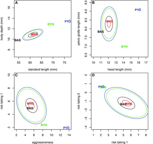
Pattern of phenotypic differentiation in selected traits. Panels A and B present two examples of morphological traits, whereas panels C and D present examples of behavioral traits. The population codes indicate the mean additive genotypes, whereas the ellipses of respective colors denote median distances of differentiation expected under random genetic drift, as inferred by driftsel. The ellipses are centered at the Bayesian estimate of ancestral mean genotype. This figure has been produced by modifying the code of viz.traits in driftsel. For interpretation of the behavioral traits, see main text.
The signal of selection in behavioral traits was clear-cut when using habitat information ( in a multivariate analysis with all traits included), but less so when ignoring it ( ; Table 1). This finding was in line with the observation that the proportions of variation explained by habitat and population are somewhat lesser for behavioral than for morphological traits (Table 1). Once the behavioral traits are investigated in more detail by analyzing different combinations or subset of traits, it becomes apparent that inclusion of habitat information (H test) increases the power to detect natural selection (Table 2). However, this finding is not to be interpreted so that the H test is unequivocally a more powerful method than the S test (see Discussion). Visual inspection of the patterns of divergence in behavioral traits (Fig. 3C, D) revealed them to be similar to those found in morphological traits (Fig. 3A, B), but at this time, both sea populations (WHS and BAS) had mean genotypes much compatible with random genetic drift. Thus, the signatures of selection in behavioral traits were weaker here.
Signals of selection in behavioral traits. Test statistic S takes into account ancestral genetic correlations and the pattern of relatedness among local populations, whereas the H statistic takes also into account habitat information (in this case, pond/marine origin). Aggressiveness = no. of attacks against a stimulus conspecific, risk taking 1 = time till the fish fully came out from a refuge in a new, potentially dangerous situation; risk taking 2 = whether fish bit on food after a simulated attack within 300 sec. Statistically significant effects are in bold
| Traits analyzed | S | H |
|---|---|---|
| Aggressiveness + Risk taking 1 + Risk taking 2 | 0.91 | 0.99 |
| Aggressiveness + Risk taking 1 | 0.93 | 0.98 |
| Aggressiveness + Risk taking 2 | 0.89 | 0.98 |
| Risk taking 1 + Risk taking 2 | 0.70 | 0.86 |
| Aggressiveness | 0.91 | 0.97 |
| Risk taking 1 | 0.71 | 0.79 |
| Risk taking 2 | 0.69 | 0.84 |
Discussion
In this article, we have developed a new analytical metric to detect signatures of past natural selection on phenotypic traits, and illustrated the use of this metric into the case study of Fennoscandian nine-spined sticklebacks. Our results show that the stickleback populations have experienced divergent natural selection especially in morphological, but also in behavioral traits. As such, the results provide formal evidence for the assertion that the phenotypic divergence observed among nine-spined stickleback populations is adaptive, which has been previously difficult to demonstrate by using QST − FST comparisons, due to a high degree of neutral baseline differentiation in marker genes among these populations (Shikano et al. 2010; Bruneaux et al. 2013). To the new analytical metrics, the results demonstrate that incorporation of environmental information into driftsel's (Karhunen et al. 2013) neutrality test can help to filter out signatures of selection in situations where they would otherwise go undetected. In what follows, we will discuss these points in more detail.
The inclusion of habitat information in the neutrality test (the new H test) increased the ability of driftsel (Karhunen et al. 2013) to detect natural selection in some cases, particularly in the case of the behavioral traits. However, caution should be exercised in drawing general conclusions on the relative merits of H and S, as these two tests focus on fundamentally different aspects of information in the data. The S test asks whether the mean population genotypes have evolved differently from what can be expected regarding the pattern of coancestry among local populations. The H test asks whether the mean genotypes correlate with the environmental covariates more than expected on the basis of the pattern of coancestry among populations. As the test statistic H uses additional information about environmental covariates, it can in some instances uncover stronger indications of selection than the test statistic S. However, this does not need to be the case. For instance, if the pattern of phenotypic differentiation among populations is due to an unmeasured environmental gradient which is uncorrelated with the measured environmental variables, H will fail to indicate selection while S may still do so. Furthermore, the H test does not ask how far the populations have diverged from the ancestral mean, so that even a high degree of differentiation can pass unnoticed, as long as it is sufficiently uncorrelated with the environmental variation. Thus, we advocate the use of both tests. As such, the new H test can be viewed to add flexibility to hypothesis testing by allowing more rigorous tests of (adaptive) parallel phenotypic evolution in any kind of metric traits. Conceptually, the H test resembles the MANCOVA procedure of Langerhans and DeWitt (2004), which takes into account the effects of habitat on population on phenotypes, but does not involve a measure of the genetic similarity between populations. By incorporating information obtained from neutral DNA, we are able to account explicitly for the influence of random genetic drift on the observed differentiation.
The H test developed here bears also some parallelism to genome scan studies devised to detect molecular footprints of natural selection (e.g., Storz 2005). These methods have evolved from generic scans for detecting signatures of selection, into approaches incorporating tests for association between selected, that is outlier, loci, and environmental variables (e.g., Coop et al. 2010; Tsumura et al. 2012). These tests are analogous to our H test in the sense that also the latter look for associations between environmental variables and footprints of selection. However, in contrast to H test, genome scan studies do not directly focus on phenotypes of interest, but markers putatively in linkage with the selected phenotypes. Nevertheless, analogously to the new generation of genome scan methods (reviewed by De Mita et al. 2013), the H test developed here can be viewed as an extension of the earlier S test (Ovaskainen et al. 2011), which in turn was built to improve traditional QST − FST approaches (see Leinonen et al. 2013).
A potential limitation of the methods used in this study is that equation (4), which forms the basis for both S and H tests, has been derived assuming that mutation rate is negligible with respect of other evolutionary and demographic forces (Ovaskainen et al. 2011). This may be a justified assumption in some cases (e.g., in case of a recently fragmented metapopulation), but we do not encourage the use of dritsel in studies which involve populations which have been subject to a very long history of reproductive isolation. We also emphasize the fact that the choice of neutral DNA markers used to estimate the degree of neutral baseline differentiation may matter (e.g., Edelaar et al. 2011): markers with extremely high mutation rates might lead into underestimation of differentiation expected due to genetic drift. A second technical limitation is that driftsel is, at present, limited to binary and normally distributed traits. Hence, further work is required, not only to explore the sensitivity of the method to its assumptions, but also to extend the sampling model by incorporating other distributional forms (e.g., Poisson and negative binomial), as many metric traits do not conform to simple normal or binomial models.
Although the earlier implementations of QST − FST comparisons typically require data from a large number of populations (O'Hara and Merilä 2005; Ovaskainen et al. 2011), the H and S tests can effectively use information also in small data sets. Indeed, in this study, strong statistical support for adaptive divergence was obtained using a very small data set comprising only 92 individuals from four populations only. Hence, apart from providing strong evidence for adaptive basis of population differentiation in nine-spined sticklebacks, our results highlight the virtues of H and S tests as a powerful and flexible approach for detecting natural selection.
Earlier studies of differentiation among marine and pond nine-spined stickleback populations have provided abundant evidence for strong, consistent, and genetically based differentiation in mean values of many morphological, life-history, neuroanatomical, and behavioral traits (reviewed in Merilä 2013). Although these differences are arguably likely to have evolved independently many times as adaptations to life in pond environments, the formal proof for natural selection being the agent behind these divergences has been lacking for all studied traits, except for body size (Shimada et al. 2011). Using the QST − FST approach, Shimada et al. (2011) showed that the body size differences between one pond and marine population exceed that to be expected on basis of genetic drift. However, the size divergence between these two populations was extreme and the conventional QST − FST approach was performing well. Here, by using the extended version of driftsel, we were able to provide formal evidence that natural selection is responsible for the divergence in body size, shape, armor, and behavior in a wider set of nine-spined stickleback populations.
In the case of the morphometric traits, the evidence for adaptive differentiation was obtained both by using S and H tests. However, in the case of the behavioral traits, S tests failed but the H test succeeded in finding statistically significant support for adaptive differentiation. This slight contrast in the results obtained for morphological and behavioral traits is consistent with the observation that habitat explains typically more of the variance in morphological traits than the population component (cf. Table 1), whereas the opposite was true in case of the behavioral traits. However, it is instructive to re-emphasize the point that high proportion of phenotypic variation explainable by population of origin cannot alone provide evidence for divergent natural selection, because such a pattern could be generated by sufficiently strong random drift too. Similarly, even though a great proportion of phenotypic variation in many traits can be explained by habitat, this can in principle result from the fact that populations in similar environments may have a shared evolutionary history. Thus, it is crucial that both S and H tests account for the influence of evolutionary history by viewing the distribution generated by neutral genetic drift as a null model.
To sum up, we have devised an improved approach to detect signatures of natural selection in quantitative traits, and demonstrated it to be suitable and powerful also in situations where the number of study populations and sampled individuals are low. We have illustrated the virtues of this approach by using empirical data on differentiation of quantitative traits among marine and pond populations of nine-spined sticklebacks—a study system where detection of signatures of natural selection with traditional methods is challenged by a high level of random drift in neutral marker genes. The method developed in this study should provide a useful framework to test for adaptive nature of population differentiation in many kinds of study systems, in particular ones with a small number of local populations or a high rate of random genetic drift.
ACKNOWLEDGMENTS
The authors thank A. Gonda for her help in collecting, rearing, and measuring the fish, as well as the numerous people who helped us in locating and obtaining fish used in this study. The authors also thank T. Shikano for access to the earlier published microsatellite data and two anonymous referees for constructive criticism which improved this manuscript. Our work was funded by Academy of Finland (Grants 200940, 108601, and 118673 to JM and 250444 to OO), and the European Research Council (ERC Starting Grant 205905 to OO).
LITERATURE CITED
Associate Editor: R. Fuller
