Deep learning formulation of electrocardiographic imaging integrating image and signal information with data-driven regularization

Abstract

Introduction

Cardiac arrhythmias often require invasive catheter measurements in order to precisely diagnose the pathology and plan the therapy. This information on the local electrical activity in the myocardium can theoretically be obtained non-invasively through electrocardiographic imaging (ECGI). Electrocardiographic imaging allows a panoramic three-dimensional visual reconstruction of the electrical activity of the heart from body surface potentials (BSP), see Figure 1. This technique requires anatomical information of the heart and torso from 3D imaging, BSP measured with electrodes and their localization on the torso surface, and mathematical methods to solve the inverse problem. Electrocardiographic imaging has been an active research area for decades. The first sketch has been proposed in 1977¹ and its history and clinical applications were recently reviewed.² Important progress was achieved but there are still scientific challenges due to the ill-posedness of the classical mathematical formulation. Therefore, this emerging modality is still at its infancy in clinical practice due to its currently limited accuracy and resolution.

Figure 1

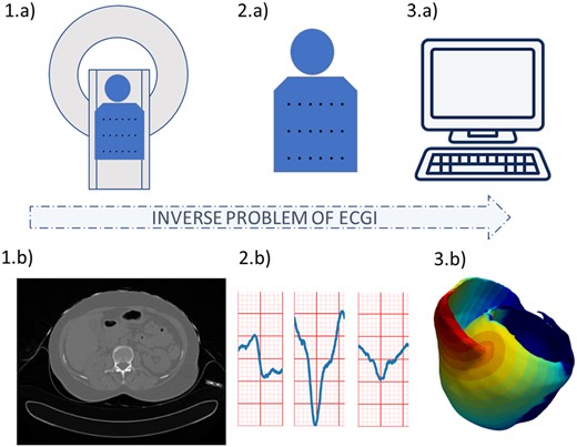
Electrocardiographic imaging process. Using (A) cardiac imaging and (B) signal processing, we obtain information on (D) the cardiac geometry and the position of the electrodes used to record the ECG signals, and (E) the surface ECG signals. Both are then used by (C) numerical methods to reconstruct the (F) cardiac electrical activity.

Open in new tabDownload slide

The classical approach is based on a transfer matrix between epicardial potentials and the torso potentials. The forward problem of ECGI refers to the computation of the electrical potential on the torso surface from the cardiac electrical activity. To compute this transfer matrix different approaches were proposed such as: the boundary element method (BEM)³ based on surfaces, or the finite element method (FEM)⁴ whereas the 3D torso anatomy is approximated by small volume elements. Both methods propagate the epicardial action potentials to the body surface with chosen boundary conditions, e.g. null current across the body surface. Ramanathan et al.⁵ demonstrated that ECGI reconstruction does not require the detailed inclusion of torso heterogeneities.

However, the inverse problem is ill-posed⁴ which means that its solution is not unique, and that its resolution will be very sensitive to noise. Small errors in input will cause large errors in the output. Therefore, a variety of formulations and regularization methods were proposed to stabilize this problem, see, for instance, the publications of the ECGI consortium (http://www.ecg-imaging.org). Recently, 15 different algorithms to solve the inverse problem were compared and the conclusion was that each of them had benefits which varied according to bi-, left-, and right-ventricular pacing.⁶ Moreover, to solve the ECGI inverse problem, it is possible to include a multitude of physiological, physical, and mathematical priors for the forward and inverse problem but also for describing the cardiac sources⁷ as well as to perform the ECG signal processing.⁸ An overview of most of these methods was published recently.⁹

However, ECGI could achieve more accurate and robust results by leveraging all the information present in the different imaging modalities acquired, as well as by introducing prior knowledge from previous cases. This is what we propose in this manuscript, through the use of deep learning (DL) and generative models.

Deep learning has generated a huge interest in healthcare applications and has become the standard method for solving a large variety of computer vision problems. Moreover, these last years, DL-based methods have proven their ability to solve inverse problems, e.g. in medical image reconstruction.¹⁰ Recently, Arridge et al.¹¹ drew up a state-of-the-art of DL approaches for solving inverse problems and has showed the benefits of such data-driven methods.Ghimire et al.¹² introduced autoencoders into ECGI for the regularization of temporal information.

Our new numerical method is based on DL and autoencoders in order to solve the whole inverse problem and reconstruct accurate 3D activation maps. A preliminary version of this method in 2D and on a single geometry was presented by Bacoyannis et al.¹³

In this manuscript, we propose to reformulate the whole ECGI problem as a β-conditional variational autoencoder based on convolutional neural networks.

Using a DL model as autoencoder trained on a large database, i.e. activations with different pacing locations, allows to get more robust methods and reduces the prediction time. The developed method was used to predict activation maps for different cardiac geometries with their corresponding simulated BSP. The model was trained and tested on a simulated database using a personalized cardiac simulation pipeline.¹⁴ Compared with the classical mathematical formulation of ECGI, this approach has five main advantages:

• Spatio-temporal correlations: the convolutional model learns interactions in space and time between signals, while most ECGI methods solve each time step independently or use a temporal prior without spatial correlations.

• Imaging substrate: the correlation between the substrate from imaging (i.e. myocardial scar) and the signals is also learned, therefore, we can seamlessly integrate any 3D image information in ECGI, while this is still difficult in the classical formulation.

• Data-driven regularization: using a generative model from a low dimensional space should ensure smooth variations between similar cases; this could alleviate the ill-posedness issue.

• Volumetric predictions: this 3D convolutional approach generates volumetric activation maps within the whole myocardium, not limited to the epicardium and the endocardium.

• Fast computations: once trained, DL methods are very fast to evaluate.

In order to achieve this, we use Cartesian grids for all the data (space and time) to leverage the power of convolutional neural networks.

In the following section, we will first present our DL model, then the method used to simulate activation maps from CT images and we will describe the computation details of our model.

Methods

Deep learning approach

We base our reformulation of ECGI on a probabilistic generative model, namely a Conditional Variational AutoEncoder (CVAE).^15,16 A CVAE is an extension of a Variational AutoEncoder (VAE)¹⁷ which is itself a powerful probabilistic generative version of autoencoders.¹⁷

An autoencoder is an unsupervised learning technique which compresses the relevant information of the input data into a low-dimensional latent code in order to reconstruct output data with the least possible amount of difference with the input. This dimensionality reduction allows to capture the more important features of the input data.

In a VAE, the term Variational refers to variational inference or variational Bayes used to approximate complex distributions. As the autoencoder, the VAE consists of two connected networks: an encoder and a decoder. The former takes an input x and compresses it into a low-dimensional latent representation, which variables are denoted z, with a prior distribution P(z), often assumed to be a centred isotropic multivariate Gaussian $P(z)=N(z:0,I)$⁠. The latter takes z as input and reconstructs the data from the generative distribution $PΘ(x|z)$⁠. This likelihood distribution $PΘ(x|z)$ is learned in the decoder neural network with parameters Θ. The resulting generative process induces the distribution $PΘ(x)=EP(z)PΘ(x|z)$⁠. Due to the intractability of the true posterior distribution $P(z|x)$⁠, the posterior is approximated by learning a simpler probability $QΦ(z|x)$ in the encoder neural network with parameters $Φ$⁠. A VAE is trained in order to maximize the probability of generating real data samples, by maximizing the evidence lower bound (ELBO). The ELBO is composed of two terms: the Kullback–Leibler (KL) divergence which is a measure between the variational probability $QΦ(z|x)$ and the true posterior distribution $P(z|x)$⁠; and the log likelihood of $PΘ(x)$ under the probability distribution $PΘ(x|z)$⁠. By minimizing the loss function, the ELBO is maximized.

Commonly, $QΦ(z|x,c)$ is Gaussian with a diagonal covariance matrix: $z∼QΦ(z|x,c)=N(z:μ,σ)$⁠, where .$z=μ+σ⊙ϵ,⊙$ denotes the Hadamard product and $ϵ∼N(0,I)$⁠.

A β-VAE intends to discover disentangled latent factors by adding a penalty coefficient on the KL divergence. Higgins et al.¹⁸ shown that with $β>1$ the model achieves better disentanglement performance than classical VAEs.

Artificial neural network architecture

The proposed method aims to generate cardiac activation maps using two constraints: the 3D imaging data of the patient heart and the BSP signals. Therefore, we use a multimodal input β-CVAE, which consists of three elements: the encoder, the latent vector, and the decoder. The architecture of our DL model is described in Figure 2.

Figure 2

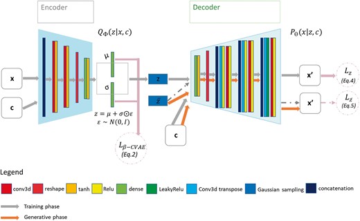
β-CVAE model architecture. Training: input data are BSP mapping signals concatenated with myocardial mask and encoded in z. Activation maps are decoded from z with conditioning by sub-sampled versions of the BSP mapping signals and of the cardiac mask. Prediction: decoder is used to generate myocardial electrical activation maps from a new cardiac segmentation and its corresponding BSP mapping signals. BSP, body surface potentials; CVAE, Conditional Variational AutoEncoders.

Open in new tabDownload slide

First, the encoder takes as input data the normalized activation maps x and as conditioning data c the BSP signals, and the cardiac image. As these data come from different modalities, BSP and imaging data do not have the same dimension. To obtain the same shape for the signals, we applied two successive 2D convolutional layers. Then these three input are concatenated to be used as a single input to the encoder model. This enables the network to directly learn spatiotemporal correlations within these input. The encoder consists of two successive convolutional layers (see Computational details section for the implementation details) following the grey arrows, which compress the input.

The 3D output of these convolutional layers is flattened to 1D before being fed to a dense layer to further compress the output vector into 16 dimensions. We then generate from it the multivariate Gaussian means and standard deviations μ and σ. In order to sample the latent vector z, we used the Gaussian re-parameterization method.

The decoder network consists of a main branch which takes the vector z as input, and the conditional branches, where the conditional input c is integrated. The main branch applies a dense layer to the input z, before reshaping the 1D vector to a 3D matrix. Then, we use the combination of transpose and normal convolutional layers at each level to increase the output dimension back to its original size. At each level, we use two convolutional layers (strided followed by non-strided) on the condition inputs c to generate the condition input in the same shape as the output from the main branch. Then, we concatenate the condition input with the main branch output. At the end of the decoder, we multiply the output with the myocardial image binary mask M to only provide predictions within the myocardial wall.

Supervised learning loss function

During the training of the CVAE, we use a modified version of the root mean squared error (RMSE), Eq. (3), to calculate the reconstruction loss.

Synthetic data generation: electrocardiographic imaging forward problem

In order to evaluate the proposed methodology, we built a synthetic database from six cardiac anatomies based on CT-scans provided by the CHU Bordeaux, France, see Figure 3. All six patients showed post-infarction scar resulting in severe thinning of the left ventricular wall. We generated synthetic electrical data with the forward problem of electrocardiography. In our case, we use a dipole formulation, assuming that the torso domain is homogeneous and infinite.¹⁹

Figure 3

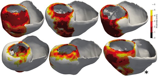
Five cardiac anatomies from CT imaging used for training and one (*) for testing. The thickness maps show the infarct scars.

Open in new tabDownload slide

Figure 4

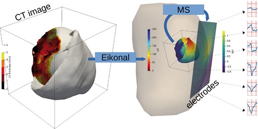
Synthetic data simulation process: myocardial wall thickness from patient image is used to parameterize the Eikonal model that generates activation maps (LAT, local activation time). The Mitchell–Schaeffer model with the dipole formulation are used to generate BSP mapping signals. BSP, body surface potentials.

Open in new tabDownload slide

For these simulations, we vary the local conduction velocity according to the local myocardial wall thickness, as chronic infarcts generate thinner walls with slower conduction velocity; this approach has been shown to efficiently reproduce intra-cardiac activation maps recordings.²⁰ For each simulation, to initialize the wave front propagation, we chose randomly a single pacing onset where the heart had a wall thickness superior to 6 mm. We defined a stopping value for the propagation at 250 ms.

In total, we simulated 6000 activation maps and the corresponding BSP using six patient image segmentations from CT images. We resampled the activation map and the myocardial wall to have the same dimensions $100×100×100$⁠. The signal input is kept at $10×10×250$⁠.

Computational details

The model was trained on five patient geometries, see Figure 4A, including a total of 5000 activation maps and their corresponding BSP, which were divided into 8 : 2 ratio for training and validation datasets. We then tested the trained model on 200 activation maps and their corresponding BSP from a new geometry unseen during the training Figure 4B. The neural network design, training, and testing were implemented using Keras API of Tensorflow 2.0 (https://www.tensorflow.org/api_docs/python/tf/keras).

To adapt the signal shape, we used two 3 × 3 2D convolutional layers with the number of strides of 2 and 5 and the number of output features of 200 and 100, respectively. The encoder of our network consists of two successive stride two convolutional layers (Figure 2), one flatten layer followed by one dense layer. Each layer has a $3×3×3$ kernel and all the activation functions are tanh. The bottleneck layers (μ, σ, z) are fully connected. From different tests, the latent code size was set to 25. The decoder has a fully connected layer which is then reshaped into a 3D matrix before applying a succession of transpose and normal convolutional layers. The model was optimized using the total loss described in Eq. (6), without any additional weight applied to the loss terms. The best value for β, the penalization term in the loss function, was 10. We used Adam²⁵ optimizer with a learning rate of $10−4$⁠, with a batch size of one for 240 epochs. The computation time for training was 64 h on a NVidia Tesla V100 (32GB of RAM).

Results

When testing the method, our probabilistic generative model allows us to generate multiple solutions from a single input, by sampling the latent space. To compare our predictions with the ground truth activation, we generated 10 different activation maps for each case and computed the mean and standard deviation of these predictions. Figure 5 shows a 3D visualization and a slice of the estimated mean activation map over the 10 predictions Figure 5B in comparison with the ground-truth simulated cardiac electrical activity Figure 5A. Figure 5C represents the standard deviation map for these 10 predictions, and Figure 5D the error map between the generated and the ground truth maps.

Figure 5

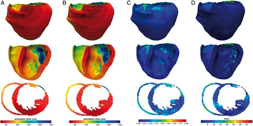
(A) Ground truth activation map, (B) activation map generated by the presented method, (C) standard deviation map calculated over 10 predictions, and (D): error-map, difference between predicted and simulated activation maps. All results are in 3D, showing the middle x-axis slice in the bottom of the figure.

Open in new tabDownload slide

We evaluated our model by testing it on a new patient anatomy over 200 activation maps. Due to the probabilistic property of our method, we predicted 10 distinct activation maps for each BSP data.

The proposed method is able to generate volumetric activation maps with a good accuracy on this simulated data: the mean absolute error is 11.33 ms with 4.10 ms standard deviation on this testing set.

Small errors and small standard deviation in Figure 5C and D indicate that the reconstruction performs well and in a consistent way, while large values mean that the reconstruction is suffering. The zones with the highest error correspond partly with the zones with the highest standard deviation in the maps. This underlines the potential use of our probabilistic generative model to help in quantifying the uncertainty in the predictions.

From the representative results shown in Figure 5, we can observe that the weight applied to the loss function influences the performance of the reconstruction in the later regions of the wave propagation. In opposition, zones where the propagation starts are better reconstructed.

Discussion

The proposed approach demonstrated great accuracy on this synthetic database with a good robustness to anatomical variations. However, the goal of this work is to apply it clinically for diagnosis and therapy planning. So, it is necessary to detail the limitations we have at this present stage in order to consider the required extensions.

To generate our database, we only considered single pacing sites. A first extension to our work will be to simulate data with multiple onsets. This is straightforward to implement, but the accuracy of the results has to be evaluated.

Second, we use the Eikonal model, which is a simplified model in terms of transmembrane potential capabilities in comparison with more complex models as the Bidomain one. However, we believe that this model can be used in many clinical cases. Indeed, the spatial dynamics of the Eikonal model and the reaction–diffusion equations are extremely similar.²⁶ The local conduction velocity modifications can represent the impact of infarcts on activation maps.²⁰ Thus, we believe that this fast method to simulate activation maps is relevant in a context of myocardial infarction. The limit of this model is reached for arrhythmias or pathologies modifying local transmembrane potential profile. From a more global and mathematical point of view, the Eikonal model provides a very strong prior on spatiotemporal correlations for solving the ECGI inverse problem.

Moreover, our method makes the hypothesis about isotropic propagation in the heart. Although heart anisotropy may not play an important role for ECGI because of the spatial scale at which it is working, we know that it has an important impact on local propagation front and thus in the forward problem. In the future, we are going to include the fibres in our forward problem formulation, which will be an easy extension.

In order to evaluate our model, we generated 10 activation maps for each case. It would be interesting for each one of these cases to vary the number of activation maps we generated and to estimate the effects on the accuracy of the model and the uncertainty quantification.

Moreover, this method has to be evaluated on real data. The differences between the training data and the testing data can severely impact performance. Robustness to signal noise and missing leads, a classical problem in ECGI, has still to be quantified. We believe that adding noise to our simulated database should help. We also intend to train the model on a wider variety of simulated data and also on some real data with partial ground-truth from catheter mapping. To help moving from synthetic to real data, we may use transfer learning.²⁷

Conclusion

Our proposed β-CVAE is able to generate a 3D volumetric map of the cardiac electrical activity for a new geometry from non-invasive BSP and cardiac imaging data. During the training, our model is designed to learn spatiotemporal as well as geometrical information. This novel formulation enables to directly introduce all the imaging information on cardiac substrate within the ECGI methodology and therefore fully exploits the available patient information.

This is the first time an ECGI method is able to reconstruct the activation pattern throughout the myocardium in a volumetric manner at such resolution, while integrating 3D substrate information from imaging and within a probabilistic framework. This promising formulation now has to be evaluated on real clinical data.

Funding

The research leading to these results has received European funding from the ERC starting grant ECSTATIC (715093) and French funding from the National Research Agency grant IHU LIRYC (ANR-10-IAHU-04). This paper is part of a supplement supported by an unrestricted grant from the Theo-Rossi di Montelera (TRM) foundation.

Conflict of interest: none declared.

Data availability

The data underlying this article will be shared on reasonable request to the corresponding author.

References