


Abstract
Effects of insecticides on terrestrial adult life stages of otherwise aquatic insects, such as mayflies (Ephemeroptera), stoneflies (Plecoptera), and caddisflies (Trichoptera), are largely unknown. In the present study, a risk model was used to pinpoint the species most likely to experience effects due to spray drift exposure during the adult life stage. Using data from an earlier case study with lambda‐cyhalothrin, 6 species with different life cycle traits were used to explore how life cycle characteristics may influence vulnerability. In addition, we performed a generic calculation of the potential effect on the terrestrial life stages of 53 species (including 47 species with unknown sensitivity). Our approach incorporated temporal and spatial distribution of both the insect and the insecticide, creating different exposure conditions among species due to variation in the relative proportion of the populations present at the time of insecticide spraying. The Ephemeroptera species represented were least vulnerable due to their extremely short adult life span and relatively short flight period. Based on their life cycle characteristics, Plecoptera and Trichoptera species were more vulnerable. These vulnerable species segregated into 2 distinct groups; one with a long adult life span to emergent period ratio and another with a high overlap between emergent period and spraying season. We therefore recommend that future ecotoxicological tests be done on species with these life cycle characteristics. Environ Toxicol Chem 2021;40:1778–1787. © 2021 SETAC
INTRODUCTION
The risk of insecticide effects on nontarget organisms involves the concentration and duration of exposure and the susceptibility of the species of concern. Susceptibility has a paramount importance for the unintended effect of insecticides. However, the occurrence of pesticide exposure may have been overlooked for some species as a consequence of their specific life cycle characteristics This problem may apply to freshwater insects such as caddisflies (Trichoptera), stoneflies (Plecoptera), mayflies (Ephemeoptera), dragonflies (Anisoptera), and damselflies (Zygoptera), because their juvenile life stage occurs in streams, ponds, and lakes, and the reproductive adult stage is terrestrial. The aquatic environment may act as a refuge from terrestrial spray drift exposure. However, exposure of terrestrial life stages to insecticide via spray drift may have paramount consequences due to effects directly impairing the recruitment for the next generation. Even though species from these insect orders share a terrestrial adult life stage, they have different life cycle strategies that may result in different spatial and temporal distributions of the populations in the terrestrial environment.
In general, adults of aquatic insects in the northern hemisphere may be found in the terrestrial environment from January to December, and emergence primarily depends on environmental factors such as light, temperature, and humidity (Williams and Feltmate 1992). However, timing and duration of the emergent period (flight period) vary considerably among species. Overall, emergence may be either synchronous (occurring over a brief period of days to a few weeks) or extended (distributed more evenly over time, lasting up to several months; see Harper 1973; Wiberg‐Larsen 2004). For these species in general, the duration of the terrestrial life stage is considerably shorter compared with their aquatic stages and varies between a few hours and several months, depending on the species. Theoretically, this creates different exposure conditions among species because different proportions of the populations are present at the time of insecticide spraying and because the likelihood of exposure for the single individual increases with duration of the adult life stage (conceptualized in Table 1).
Outline of the possible population effects of significant insecticide exposure dependent on duration of flight period and individual life span for terrestrial life stages of aquatic insects
| Individual adult life span | ||
| Emergence period | Short | Long |
| Emergence synchronized | Detrimental if exposed but with lower probability of exposure than species with long life span | Detrimental if exposed and with a higher probability of exposure than short‐lived species |
| Continuous emergence over a longer period of time | Only a small part of the population affected in case of a single exposure event, but with a higher probability that exposure will occur than for synchronized populations | Higher probability of exposure than species with short life spans, and a smaller fraction of the population will be affected in case of a single exposure event than for synchronized populations |
The differences in timing and duration and their spatial distribution among aquatic insect species may result in different species‐specific vulnerabilities, depending on exposure risk, intrinsic sensitivity, and potential for population recovery (De Lange et al. 2010). Recently, an adult stage risk indicator (ASRI) was introduced allowing estimation of ecological vulnerability for terrestrial life stages of aquatic species (Sørensen et al. 2020). This approach incorporates both temporal and spatial distribution of insect populations and pesticides as well as exposure risk and sensitivity of the insect species. Except for the study by Bruus et al. (2020) on the sensitivity of 6 species of adult insects to lambda‐cyhalothrin and imidacloprid, sensitivities of terrestrial adult stages of aquatic insects to insecticide exposure have not been quantified, as pointed out by Rasmussen et al. (2018).
The present study uses a modified ASRI with the aim of pinpointing species for future ecotoxicological testing, by assessing the vulnerability of a range of aquatic insect species with different life cycle characteristics.
MATERIALS AND METHODS
First, published data from the 6 aquatic species with established ecotoxicity data for the adult stage (Bruus et al. 2020) were used in exposure risk calculations to explore how life cycle characteristics may influence vulnerability. Subsequently, we performed a generic calculation of the vulnerability of a range of species differing in their life cycle characteristics, to identify and suggest candidate species with a high potential risk of adverse effects for future ecotoxicity studies. In this calculation, sensitivity and exposure areas were harmonized because these 2 parameters were unknown and because the generic values were needed to identify the species most likely to be exposed to spray drift due to their ecology. This was done by assigning the same size (exposure area = 40 mm2) and sensitivity (median lethal dose [LD50] = 1 ng individual–1) to all species, including the model species, for which we had data on susceptibility to one insecticide (lambda‐cyhalothrin).
Potential ecological vulnerability of species with known sensitivity
We studied 6 model species: the mayfly Ephemera danica (Müll.), the stoneflies Leuctra fusca (L.) and Nemoura cinerea (Retz.), and the caddisflies Hydropsyche angustipennis (Curt.), Agapetus ochripes (Curt.), and Anabolia nervosa (Curt.). These 6 species have all previously been tested for sensivity of the adult stage to 2 insecticides, lambda‐cyhalothrin and imidaclorid (Bruus et al. 2020). A short ecological description of each species, including life span and central ecological and behavioral characteristics relevant for assessing the potential ecological vulnerability at the population level, is presented in the following paragraphs.
Ephemera danica is a large mayfly with an adult body length of 18 to 22 mm. The juvenile life stages last for 1 to 3 yr in total, depending on the abiotic environment (Svensson 1977; Vilenica et al. 2017). Despite this variance in life span, the emergence of the adults is rather coordinated (Svensson 1977), because the emergence period only lasts for a few weeks, ranging from late May to early June (Svensson 1977; Bennett 2007). Neither of the 2 adult life stages (subimago and imago) actively feed (no alimentary canal present in mayflies), and, consequently, the duration of the adult life stages is short (2–3 d). Male E. danica have coordinated male swarming in relation to mating.
Leuctra fusca has an adult body length of 5 to 8 mm and a univoltine life cycle. The primary emergence period is August to October (Lillehammer 1988). The adult stage lasts for approximately 2 to 3 wk. Adults feed on algae on tree branches.
Nemoura cinerea has an adult body length of 5 to 11 mm and a univoltine life cycle. The emergence period is May to August (Bengtsson 1972; Lillehammer 1988), but may occasionally be even longer (Hynes 1977). In general, the adult life span is 2 to 3 wk, but may extend further under optimal growth conditions (Hynes 1942). Adults feed on detritus, algae, and cyanolichens (De Figueroa and Sanchez‐Ortega 2000).
Hydropsyche angustipennis has an adult body length of 10 mm and a univoltine life cycle. The emergence period lasts from late June to early September (Wiberg‐Larsen 2004). The adult stage lasts for 1 to 2 wk in nature and, most likely, they do not feed. During mating, the males swarm over geographical markers such as bushes and trees to attract females (Brindle 1957; Benz 1975).
Agapetus ochripes is a small caddisfly with an adult body length of approximately 4 mm. The life cycle is univoltine, and the emergence period lasts from late May to late June (Crichton et al. 1978). The adult life stage lasts for <1 wk and, most likely, they do not feed.
The caddisfly A. nervosa has an adult body length of 11 to 12 mm and the life cycle is univoltine. Under temperate conditions, the emergence period is September and October, with the adult life span being approximately 1 mo (Wiberg‐Larsen 2004). The adults feed on available nectar sources (P. Wiberg‐Larsen, unpublished data).
Vulnerability index (ASRI)
To include the importance of life cycle traits (duration and timing of species' flight periods and individual life span) for quantifying the risk of insecticide effects, the ASRI was calculated according to Sørensen et al. (2020). A description of how the calculations were performed follows in the next paragraph.
The ASRI combines toxicity with exposure to form a relative measure of risk composed of the following 3 factors: 1) the toxic potential (), defined below; 2) coincidence between the spatial distribution of the insect population and the spatial distribution of pesticide deposition due to spraying activity ; and 3) coincidence between the temporal distribution of insect populations in the terrestrial environment and temporal distribution of the pesticide deposition (). Jointly, these factors constitute the adult stage risk indicator (ASRIi,j):
where i and j denote insect species or taxon i and active ingredient j, respectively.
Toxic potential
The is calculated as the label rate of the active ingredient j multiplied by the surface area of the individual species prone to exposure (InsectArea) divided by the toxicity of the active ingredient j on insect i measured by the mass active ingredient of pesticide/insect causing an average of 50% mortality in an acute test ():
where FullDose is ng cm–2 active ingredient sprayed at label rate, InsectArea is the exposed insect area in mm2, and LD50 is ng active ingredient of pesticide/insect. Compared with the original version of ASRI (Sørensen et al. 2020), we have added a factor that accounts for different exposure area of the species.
Spatial distribution of exposure
The spatial distribution of the insect population is described as a probability distribution for an individual to be located x meters from the edge of a freshwater system () given that the insect is alive and in its terrestrial stage. A maximal distance from the freshwater system (R) is assumed, above which the insect will not fly and return to the water system. The spatial distribution of the deposition of the active ingredient j is described by the function , and the effective exposure at distance x is estimated as the product between the probability of the individual insect i to be at distance x and the deposition of the active ingredient j at distance x. The coincidence between insect abundance and spray deposition is calculated by integrating the product between and from the edge of the water system (x = 0) at all x values up to a maximal distance R:
The lateral distribution of stoneflies, caddisflies, and mayflies has been investigated, employing malaise traps, by Petersen et al. (2004), and the recorded data disclosed relations between distance to the river or stream bank (x) and the abundance of insects. The outcome was an empirical relation between distance and abundance for different insect families and for different landscape types along the bank. The probability density distribution for abundance at distance x from the river or stream bank is therefore calculated by
where the relationship between and is obtained by assuming that the total probability of an insect being present in any distance less than Ri is 1.
In some cases, there will be an unsprayed zone along the edge of the freshwater systems with a width of Lj meters. Pesticide may drift into this unsprayed zone, and the fraction of drift compared with the dosage level is assumed to follow a hyperbolic function:
where d0 is the fraction of deposition just outside the spraying zone at x = Lj, and the parameter a measures the decrease in the amount of active ingredient with distance from the sprayed field. Both d0 and a are assumed to be independent of properties of the active ingredient, but instead depend on the physics of spraying, the local climate, and the landscape roughness. In this version of the ASRI, the d0 and a values are estimated using measured deposition data from the study by Løfstrøm et al. (2013; Figure 1). This represents deposition from a ground rig with a specific set of technical and environmental conditions, that is, a spray volume of 300 L ha–1, boom height of 0.5 m, sprayer speed of 7 km h–1, nozzle AI 110 04 at 0.3 MPa, wind speed of 4 m s–1 at 4 m, relative humidity 60%, air temperature 15 °C, heat flux 100 W m–2, and aerodynamic roughness of 0.1 m. Use of other equipment and spraying under another set of weather conditions can influence this relationship.

For insects located inside the sprayed zone (for x > Lj), the deposition is simply unity corresponding to the maximal dosage level.
It is now possible to calculate Equation 3.
Temporal distribution of exposure
The temporal distribution was calculated by integration over an entire year of the joint probability for both spraying to take place and the insect to be present as an adult at the same time:
where describes the probability density function for a spraying event with active ingredient j at time t. estimates the seasonality of spraying, where spraying will be more or less likely depending on the demand of pest control. In the indicator, the probability of spraying is calculated for intervals of days having constant probability, for example, if the probability of spraying is 0.6 for June as a whole, then the probability of each day is 0.60/30 = 0.02. Within each interval of days, the probability density is, thus, assumed to be evenly distributed within June, that is, having identical values/day. All sprayings are defined to take place during 1 yr, yielding:
The function in Equation 9 is the probability of an insect being adult and alive at time t given that this insect will emerge during the year. This probability depends on the probability of the insect emerging and its life span as an adult, also denoted flight time (Ti), and the probability will equal the probability of an insect having emerged historically in the period back in time up to Ti:
where the function is defined as the probability density function of the probability emerging at time . The rationale for Equation 11 is that the number of adult insects at time t includes all the insects that have emerged in the time period back in time, that is, from t – Tfi to t.
The function is not a probability density function, but instead describes the probability that an insect will be alive as an adult at time t under the condition that emergence will take place during the year. This simple model assumes a fixed life span, where all insects are alive during the entire time interval Ti. The total area under the curve is equal to the flight time ():
Equation 11 can be divided up into 2 integrals as:
and assuming to be modeled as a normal distribution, Equation 13 has the following form:
Equation 14 may be inserted in Equation (9).
Table 2 presents species‐specific parameter values for sensitivity, lateral distribution, life length, and flight period used in the calculation of the ASRI for the 6 model species.
Laboratory median lethal dose (LD50) values for effects of lambda‐cyhalothrin, distribution of adult specimens, life length as adult (TL), timing of the flight period, and length of emergent period (TF)a
| Order | Species | LD50b (ng a.i. individual–1) | Lateral distributionc | TL (d) | Flight period (start and end d) | TF (d) | |
| Trichoptera | Anabolia nervosa | 0.153 | 0.301 | 1.13 | 14 | 260–294 | 34 |
| Hydropsyche angustipennis | 0.42 | 0.301 | 1.13 | 7 | 139–257 | 118 | |
| Agapetus ochripes | 0.008 | 0.301 | 1.13 | 5 | 157–191 | 34 | |
| Plecoptera | Leuctra fusca | 0.11 | 0.133 | 0.772 | 21 | 251–349 | 98 |
| Nemoura cinerea | 0.026 | 0.133 | 0.772 | 21 | 129–219 | 90 | |
| Ephemeoptera | Agapetus danica | 6.17 | 0.142 | 0.797 | 3 | 260–294 | 30 |
The distribution of adult specimens with distance to watercourse is described by the following equation (Equation 4) for each order of insect. The timing of the flight period is given as the start and end days of the flight period, in days since January 1.
From Bruus et al. (2020).
From Petersen et al. (2004).
Insect surface area assessment
The total surface area of the individual species prone to exposure (InsectArea) was determined from pictures of individuals at rest. The calculation differed between taxonomic groups, because they have different resting postures and different wing characteristics. Mayflies keep their wings folded above the body, exposing both body surface and wings. The exposed area is calculated as the combined lateral surface of the head, thorax, abdomen, and wings; all were multiplied by 2 to represent both sides of the insect. The area was determined as a polygon with ImageJ (US National Institutes of Health) from digital pictures. Caddisflies hold their wings roof‐like and, consequently, the area of exposure is the double size of an average forewing size and the surface of the head. Stoneflies hold their wings flat at the top of the body. Therefore, the exposed area is determined as a half cylinder, based on the width of the body and the length of the body and wings all together. It is only a half cylinder, as the upper side of the insect shields the underside. For the present study, it was assumed that the majority of the insects will be found resting in the vegetation and only fly occasionally.
Distance between agricultural field blocks and watercourse
The calculation of the ASRI uses the parameter Lj (Equation 6), which is the distance between the border of the sprayed field and a freshwater body. This parameter determines how large a fraction of the adult population is exposed to the insecticide and the degree of exposure. To quantify these, a geographic information system (GIS)‐based landscape analysis was used to characterize the proportion of noncrop area for a number of zones with increasing distance to the freshwater body. The mean distance and variation in distance from agricultural fields to rivers and streams was assessed. A number of buffer zones around rivers and streams were used to divide the area with cultivated land into zones with increasing distance to rivers and streams. For each section of a river or stream, the distance to cultivated land was taken as the mean distance to the nearest buffer zone. In total, Denmark has approximately 64 000 km of rivers and streams; 16 000 km of these rivers and streams lie within 20 m from cultivated areas, where pesticides might be applied. For these 16 000 km of rivers/streams, the average distance from the edge of the water body to areas where pesticides may be applied was approximately 4 m.
The average distance between the field and the freshwater body (Lj) was therefore assessed to be 4 m.
Temporal distribution of exposure
Insecticides are used with different timing and intervals, depending on the crop grown and the occurrence of pests. The probability of spraying insecticides was assessed for a decision support system developed for farmers, specifically for each crop (Department of Agroecology, Aarhus University 2020). The probability of insecticide treatment over time was determined based on the treatment period suggested in this decision support system and the total area of the crops where insecticides are used. Data were aggregated on half‐month intervals. Therefore, they are not use patterns from specific agricultural fields next to streams but general descriptions. The major spraying period (highest probability of occurrence of a spray event) occurs from days 105 to 196 following January 1, summing up to a 79.4% probability of spray occurrence in this period. In addition, there was a temporally distinct autumn spraying. The result can be seen in Figure 2.
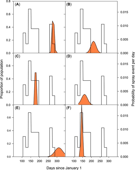
Relative occurrence of insecticide treatment from agricultural use within 1 yr and the flight period (presence of population over time presented with orange shading) for the 6 model species. The right y‐axis represents the daily probability that an insecticide spray event will occur. The species studied are shown, with the cumulative exposure probability (CEP) value given in parentheses after the species name in this figure legend. (A) Anabolia nervosa (0.20). (B) Hydropsyche angustipennis (0.60). (C) Agapetus ochribes (0.31). (D) Nemoura cinerea (0.68). (E) Leuctra fusca (0.21). (F) Ephemera danica (0.38).
Vulnerability of 6 model species
The ASRI was calculated for the 6 model species. However, because the intrinsic sensitivity of the model species was highly variable, it was hard to identify the effect of both life span and flight period length on the risk of insecticide effects, because the index integrates their interactions. The latter include interactions between early development and the degree of emergence over time, combined with the lifetime of the emerged individuals. Furthermore, the spatial distribution of the population and the likelihood of insecticide spray event are combined with the spray drift.
To determine which factor contributed most to the ASRI value, linear regression analyses were performed between single parameters or in combination and the indicator value for the 6 model species without ecotoxicological measures. This was done by assigning the same size (exposure area = 40 mm2) and sensitivity (LD50 = 1 ng individual–1) to all species. The parameters were life span, flight period, and cumulative exposure probability (CEP). The relationship between life span and flight period is important because the longer the adult life span is compared with the flight period, the larger a proportion of the total population of adults is potentially exposed/affected. The temporal co‐occurrence of an insect compared with the probable spray events is calculated as follows:
where P(spray) is the probability of a spray event occurring on a given day and P(present) is the probability that a species is adult on a given day.
Vulnerability of species of unknown sensitivity and exposure area
The potential ecological vulnerability of 47 additional species belonging to the insect orders Trichoptera, Plecoptera, and Ephemeroptera (Supplemental Data) with different adult life spans and temporal occurrences and length of the flight periods was assessed. The ASRI values were calculated as just described in the Vulnerability of 6 model species section, except that generic values were used for all species (i.e., exposure area = 40 mm2 and LD50 = 1 ng individual–1), because the area of exposure and sensitivity were unknown.
RESULTS
Temporal co‐occurrence of insects and insecticides for 6 model species
The CEP for the 6 model species showed that H. angustipennis and N. cinerea had the highest values (Figure 2B and D). It was also evident that 2 species (L. fusca and H. angustipennis) had long periods of their flight period during which no insecticides were used, whereas the other 4 species had flight periods that coincided with the main spraying period. Species with the main flight period in autumn had the lowest level of CEP (Figure 2A and E).
Insect surface area
We found large differences in surface area, with E. danica and L. fusca having the largest and smallest surface areas, respectively (Table 3).
Total surface area relevant for exposure to insecticide spray drift when resting (InsectArea in Equation 2; areas determined from single pictures of specimens)
| Species | Order | Total surface area (mm2) |
| Agapetus ochripes | Trichoptera | 16.5 |
| Anabolia nervosa | Trichoptera | 100.3 |
| Hydropsyche angustipennis | Trichoptera | 36.3 |
| Leuctra fusca | Plecoptera | 13.4 |
| Nemoura cinerea | Plecoptera | 21.3 |
| Ephemera danica | Ephemeroptera | 362.0 |
Vulnerability
We found large differences in the ASRI values for the 6 model organisms, N. cinerea having by far the highest value followed by A. ochripes and A. nervosa (Table 4). The ASRI values for the 6 test species showed no obvious trend relative to life span and flight period (Table 4). The table shows that when the intrinsic sensitivity was harmonized by adding generic values for toxicity and surface area of all species, the indicator values seem more similar within life cycle categories than prior to harmonization, albeit with large variation (Table 4). To illustrate the most important ecological parameters selected, ecological parameters were compared with the ASRI value. A linear regression analysis showed that 3 combined parameters, that is, TL (life span), TF (emergent period), and CEP, describe 92% of the variation of the ASRI values for the 6 model species (ASRI = 34.69 × (CEP × TL/TF) – 0.928, n = 6, and R2 = 0.917, p < 0.003) and 84% for the additional 47 species (ASRI = 19.38 × (CEP × TL/TF) – 0.017, n = 47, and R2 = 0.836, p < 0.001), when identical sensitivity to the model insecticide was assumed (Figure 3).
The adult stage risk indicator (ASRI) indicator value according to the life cycle characteristic of the 6 speciesa
| Adult life span | ||||
| Short | Long | |||
| Flight period | Species | ASRI | Species | ASRI |
| Short | Ephemera danica | 1.47 (1.05) | Anabolia nervosa | 17.23 (1.15) |
| Agapetus ochripes | 38.42 (0.81) | |||
| Long | Hydropsyche angustipennis | 0.33 (0.17) | Leuctra fusca | 1.21 (0.40) |
| Nemoura cinerea | 93.52 (4.57) | |||
Numbers in parentheses are the ASRI values when exposure area and sensitivity are assumed to be the same for all species.
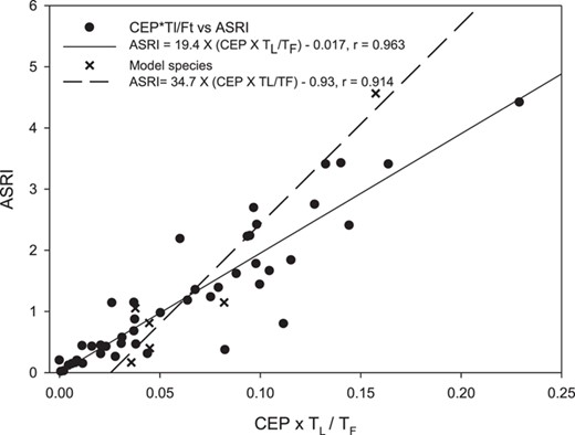
Relationship between the cumulative exposure probability (CEP) × TL/FT product and adult stage risk indicator (ASRI) for the 6 model species and the additional 47 species, respectively.
Identifying species with highest potential ecological vulnerability
The 30% of insect species with the highest indicator value segregated into 2 distinct groups: one with a high coincidence between individual life span and species flight period (TL/TF) and another with a high overlap with the spraying season (CEP; Table 5). Among the 3 represented taxonomic groups, Ephemeroptera were the least vulnerable. The Ephemeroptera species we studied have both a short flight period and a short adult life span. The Plecoptera species are among the 30% most vulnerable insects, because they have a life history that results in a high overlap with the intense spraying period. Finally, the Trichoptera species with high ASRI values generally have a long adult life span relative to flight period, with 2 distinct exceptions, Potamophylax nigricornis and Plectrocnemia conspersa. They have a flight period of 105 and 166 d, respectively, that covers the main spraying season and CEP values of 0.91 and 0.70.
Life span (TL, d), flight period (TF, d), cumulated spray probability (CEP), TL/TF, and adult stage risk indicator (ASRI) for the upper 30% of species with the highest ASRI value out of 53a
| Family | Species | TL | TF | CEP | TL/TF | ASRI |
| Plecoptera | Nemoura cinerea | 21 | 90 | 0.68 | 0.23 | 4.57 |
| Plecoptera | Isoperla grammatica | 21 | 60 | 0.65 | 0.35 | 4.42 |
| Trichoptera | Micropterna sequax | 56 | 107 | 0.27 | 0.52 | 3.43 |
| Plecoptera | Brachyptera risi | 14 | 60 | 0.70 | 0.23 | 3.41 |
| Plecoptera | Nemoura flexuosa | 14 | 60 | 0.57 | 0.23 | 3.41 |
| Plecoptera | Protonemura meyeri | 14 | 61 | 0.55 | 0.23 | 2.75 |
| Trichoptera | Limnephilus lunatus | 42 | 91 | 0.21 | 0.46 | 2.70 |
| Plecoptera | Leuctra nigra | 10.5 | 74 | 0.69 | 0.14 | 2.42 |
| Trichoptera | Oligostomis reticulate | 14 | 30 | 0.31 | 0.47 | 2.41 |
| Plecoptera | Leuctra hippopus | 10.5 | 76 | 0.69 | 0.14 | 2.24 |
| Trichoptera | Potamophylax nigricornis | 14 | 105 | 0.70 | 0.13 | 2.22 |
| Trichoptera | Chaetopteryx villosa | 42 | 80 | 0.11 | 0.53 | 2.19 |
| Trichoptera | Plectrocnemia conspersa | 21 | 166 | 0.91 | 0.13 | 1.84 |
| Trichoptera | Ironoquia dubia | 14 | 29 | 0.20 | 0.48 | 1.78 |
TF is part of the CEP calculation. The parameters with the strongest relationship to the ASRI indicator are marked in bold.
DISCUSSION
Six model species
For the 6 model species, the ASRI index differed among species, and the differences in intrinsic toxicity overruled the importance of differences in life cycle characteristic, at least for the one insecticide used in the present study—lambda‐cyhalothrin. We are aware that the sensitivity among species to this insecticide cannot be used as an approximation for relative toxicity to other insecticides (Mian and Mulla 1992; Hamer et al. 1998; Bruus et al. 2020). Consequently, there is an urgent need to establish ecotoxicity data for this species group for other insecticides, especially the most frequently applied pesticides.
The use of a vulnerability index to describe differences among species will inevitably involve simplifying the effect assessment. Some of the simplifications used in the presented index are discussed below.
Species have different activity patterns, and spraying activity is unevenly distributed over the day. Some male Ephemeropterans and Trichopterans may swarm in the afternoon or early evening, whereas many Trichopterans are mainly night active. Therefore, the diurnal pattern of the concerned species might affect the probability of being exposed. However, this is not included in the risk model due to lack of knowledge of these patterns and their relation to the timing of spraying. In addition, weather (temperature, wind speed, precipitation) influences their activity.
In addition to the direct topical exposure we considered, residual and oral uptake might be important for a more realistic toxicity assessment. This holds true especially for those species that feed on algae, other organisms, or honeydew on plant surfaces (De Figueroa and Sanchez‐Ortega 2000; Rua et al. 2017) as well as carnivorous species. These generally have a longer adult life span than nonfeeding taxa, and may even be found beyond the riparian zone in their search for food. They may be exposed not only by direct exposure, but also by residual uptake as well as an oral route. A range of studies done on very different groups of arthropods shows that pyrethroid insecticides may be repellent (Hebeish et al. 2010; Spindola et al. 2013; De Fernandes et al. 2016). This may reduce residual exposure, because the insects avoid treated/exposed surfaces. However, insects may also increase activity if they encounter surfaces with adhered pyrethroids (Alzogaray et al. 1997; Rose et al. 2006; Prasifka et al. 2008), which points to an increased residual uptake. For a specific risk assessment, including both residual and oral exposure, this may diminish the differences in vulnerability between species. We have assumed that insecticide droplets impinging on an insect have the same effect, regardless of where the droplet is deposited. However, this may not be a correct scenario for all species. The Plecoptera species hold their wings flat at the top of the body, almost covering it from above and, thus, protecting against some of the insecticides being deposited. Hoang et al. (2011) showed that for butterflies, the toxicity of the impacted insecticide depends on where it is deposited. Thus, a droplet that lands on the wings has approximately one‐fourth of the potency of droplets landing on the body (Hoang et al. 2011). On the other hand, insecticide droplets may also wash off in Trichoptera species that hold their hairy hydrophobic wings roof‐like at rest.
It is unknown how specimens allocate time between flight and rest. In the present study, we assumed that the majority of the insects are found in the vegetation and only fly occasionally. The data on spatial distribution of the adult insects primarily cover samples taken by nonattractant malaise traps. Therefore, the distribution of flying insects is representative of the spatial distribution of the insects. The experiments (Petersen et al. 2004) do not describe the long‐range dispersal, because the traps were positioned no >75 m from a water body. Thus, it is well documented that minor parts of aquatic insect populations (Plecoptera, Ephemeroptera, and Trichoptera) exhibit long‐range dispersal on the scale of kilometers (see Mendl and Müller 1974; Svensson 1974; Kovats et al. 1996; Briers et al. 2004; Wiberg‐Larsen and Nørum 2009). Such long‐range dispersal may counteract possible insecticide effects on populations, if sufficient numbers of egg‐bearing females reach the area from unexposed stream sites. However, egg‐laying must be successful, meaning it must result in a number of offspring sufficient to account for the generally high mortality during subsequent juvenile stages and adult reproduction. In addition, unexposed habitats need to be so close that the adult insects are likely to reach the exposed stream site. Therefore, because recovery also depends on favorable conditions (air temperature, direction and speed of wind), successful recolonization is not expected to be common within a short time scale, but may take several years (Wiberg‐Larsen and Nørum 2009).
The GIS analyses we performed verify that many agricultural fields were found in the immediate vicinity of watercourses. For ASRI, it was assumed that the adult individuals were distributed as observed by Petersen et al. (2004). However, we do not know to what extent the crop edge blocks the dispersing individual. In case cropped areas do act as barriers, this would result in reduced exposure (fewer individual in treated fields).
Species with long flight periods are generally univoltine (one life cycle within one season). However, some Ephemeroptera are bi‐ or multivoltine (Elliott and Humpesch 2010), a pattern that is especially common in the species‐rich aquatic family Chironomidae (Diptera; Tokeshi 1995). Insecticide impact in the early season may therefore affect the size of the late season populations and, consequently, the relative impact is underestimated by ASRI.
Vulnerable species for ecotoxicity testing
The aim of our study was to use the ASRI index to pinpoint species for future ecotoxicological testing. We found distinct differences in vulnerability response patterns among the taxonomic groups we studied, Ephemeroptera, Plecoptera, and Trichoptera. Ephemeroptera have a very short adult life span as well as a short flight period. This means that they do not have a high CEP, even if the flight period coincides with the main spray season, because the short presence minimizes the overall probability of a co‐occurring spray event. Their adult life span is so short that the TL‐to‐TF ratio is low. Therefore, these species have a low risk of exposure and, in case of exposure, only a small fraction of the adult population is affected. Plecopteran and Trichopteran species have a life history that results in a high overlap with the main spray period. They have a long flight period, but not a comparably long adult life span, although some Trichopteran species with summer diapause may live for 4 to 6 mo (Svensson 1972).
The ASRI values we have presented suggest that species with a high overlap with the spraying season or a high life span‐to‐flight period ratio are the most relevant to use in the process of determining the sensitivity of terrestrial life stages of freshwater insects. The reason is that they have the highest vulnerability.
Finally, the present study only deals with the risk of effects on the adult terrestrial life stage. It cannot be ruled out that the juvenile aquatic life stages may be exposed to insecticides due to spray drift, overspray, or wash‐out from the soil or drainage tubes. In these cases, the adults may have an altered sensitivity or the population may diminish during the juvenile stage. An integration of risks to both juvenile and adult life stages would therefore be needed for a thorough risk assessment.
CONCLUSIONS
Terrestrial exposure may be hazardous for multiple taxa of Ephemoptera, Plecoptera, and Trichoptera. We found that the ASRI not only describes the vulnerability, but also can help to identify critical parameters for vulnerable species. The present study describes the potential effect on the terrestrial life stage; however, knowledge gaps remain: Aquatic and terrestrial parts of the life cycles should not be seen as isolated entities, and there is a need to investigate whether aquatic exposure leads to a higher sensitivity in the terrestrial stage and vice versa.
Supplemental Data
The Supplemental Data are available on the Wiley Online Library at https://doi.org/10.1002/etc.5025.
Acknowledgment
The authors thank anonymous reviewers and the editor for valuable and constructive comments received on an earlier version of the manuscript.
Author Contribution Statement
C. Kjær and P.B. Sørensen conceived the study; P. Wiberg‐Larsen qualified the ecological parameters for the single species; J. Bak performed the GIS analyses; P.B. Sørensen made the model calculations with assistance from C. Kjær; C. Kjær led the writing of the manuscript, and all co‐authors contributed to revisions.
Data Availability Statement
Data, associated metadata, and calculation tools are available from the corresponding author ([email protected]).
