


Abstract
This study explores how agrobiodiversity at both local and regional scales impacts farmland value across five Mediterranean countries in the EU. Previous literature has primarily addressed on-farm biodiversity and its effects on productivity and risk mitigation, yet the potential externalities of agrobiodiversity across neighboring farms remain underexplored. Using a cross-sectional Ricardian approach, we estimate the effects of agrobiodiversity, measured in terms of both crop richness and evenness, on long-term agricultural productivity. Our findings show significant non-linear relationships and substitution effects between local and regional agrobiodiversity, underscoring the need for regionally tailored biodiversity policies.
1. Introduction
Biodiversity conservation is increasingly seen as a key to maintaining and enhancing the provision of ecosystem services (Johnson et al., 2021; Dasgupta, 2021). Within agricultural landscapes, diversity provides multiple ecological benefits, including improved soil health, enhanced water retention, and natural pest control, all of which directly contribute to farm productivity and profitability (Power, 2010; Landis, 2017).
Agrobiodiversity is increasingly acknowledged as a critical factor in promoting ecosystem services that underpin sustainable agricultural production (Jackson, Pascual and Hodgkin, 2007; Foley et al., 2011). This diversity is crucial not only for crop resilience and productivity but also for enhancing the overall ecological health of agricultural systems (Swift, Izac and van Noordwijk, 2004; Tamburini et al., 2020). Different agricultural land cover types interact to create habitat heterogeneity, which can support biodiversity at multiple trophic levels and foster ecosystem functions essential for crop production (Tilman et al., 2001).
Numerous studies have shown that agrobiodiversity supports ecosystem functioning, which can enhance yields and yield stability (Isbell et al., 2011, 2017). In addition, economic studies have found that on-farm diversity increases productivity and farm viability (Di Falco, Bezabih and Yesuf, 2010; Chavas and Di Falco, 2012; Noack and Quaas, 2021). However, agroeconomic systems may also rely on the local biodiversity of nearby farms for some ecosystem services such as pollination, biological control of pests, and nutrient cycling (Garibaldi et al., 2018). Also at the local level, crop mosaics promote ecosystem services and benefit crop production (Duflot et al., 2022). At a larger scale, heterogeneous composition of agricultural landscapes can make the regional system more stable against environmental and economic risks (Loreau, Mouquet and Gonzalez, 2003; Isbell et al., 2011, 2017). Studies tackling the economic impact of crops diversity emphasise the existence of a trade-off between the gains from specialisation at farm-level and reducing the risk of crops failure at the aggregate level (Weitzman, 2000; Bellora and Bourgeon, 2019).
This paper uses a cross-sectional Ricardian approach (Mendelsohn, Nordhaus and Shaw, 1994) to explore whether farmland value (long-run agricultural profitability) is affected by local and regional agrobiodiversity. The local index is measuring whether agrobiodiversity influences ecosystem services that can act as positive or negative externalities for nearby farms. The regional measure is asking a broader question concerning what portfolio of farmland cover leads to the highest farmland value.
Biodiversity encompasses various dimensions that can be measured in multiple ways. Landscape compositional complexity and landscape configurational complexity are two key concepts in landscape ecology used to describe the structural diversity of landscapes. The former refers to the variety of land cover types within an area, while the latter focuses on their spatial arrangement. Although both aspects are crucial for understanding how landscapes influence ecosystem services, compositional complexity has been found to have a stronger and more consistent impact on crop productivity (Nelson and Burchfield, 2021).
Purvis and Hector (2000) categorise commonly used biodiversity measures into three conceptually distinct approaches, each capturing a unique facet of biodiversity: richness, evenness and difference. These approaches, though interconnected, offer distinct insights into biodiversity.
In our analysis, we incorporate all three categories: the richness (or number) of agricultural land cover types, their evenness (or relative abundance distribution) and the spatial difference between local and regional levels of agrobiodiversity. By addressing these dimensions, we aim to provide a comprehensive assessment of agrobiodiversity’s impact within agricultural landscapes.
Most previous studies on the productive value of crop diversity focus on field- and farm-level analyses, with only a few examining the impact of agrobiodiversity at a broader scale. Di Falco and Chavas (2008) and Donfouet et al. (2017) explored whether regional agrobiodiversity can buffer against adverse climatic conditions. Both studies utilised a production function approach to assess the influence of regional diversity on agricultural output in Southern Italy and France, respectively, using the Shannon diversity index. Their findings suggest that diversity enhances production, particularly under low or limited rainfall conditions within the agroecosystem. Similarly, Bellora et al. (2018) observed a significant, albeit heterogeneous, impact of the Shannon index of crop diversity across different landscape scales. Their results reveal that the effect of diversity is generally positive and diminishes with scale, although they also detect a negative impact at larger landscape levels for certain crops, underscoring the heterogeneity of crop diversity effects across crops and scales. Burchfield, Nelson and Spangle (2019) analysed the effects of county-level agrobiodiversity measured by the richness index, the Shannon diversity index and the Simpson diversity index on the log of yields of selected crops in the USA. Their findings highlight notable differences in yield responses to these diversity metrics, showing minimal response to increases in the Simpson diversity index, a positive response to high levels of richness, and a convex response to the Shannon index—mostly negative, becoming positive only at higher values.
While previous research has primarily focused on crop diversity’s impact on productivity (measured by yield or gross production), biodiversity may also support ecosystem services that can substitute for manufactured inputs, as demonstrated by Bareille and Dupraz (2020) and Bareille and Letort (2018). This substitution effect can reduce variable costs, suggesting that measures of profitability, such as net revenue, provide a more comprehensive assessment by capturing these additional economic benefits associated with biodiversity. For example, Auffhammer and Carleton (2018) examined the impact of crop concentration on gross revenue, net revenue and yield at the district level in India. They found that while higher crop diversity reduces sensitivity to adverse weather events across all three metrics, only net revenue directly reflects the positive effects of crop diversity.
This study is the first empirical analyses to examine the relationship between farmland value and both local and regional agrobiodiversity, as well as the interaction between them. The exploration of crop heterogeneity’s contribution to agricultural productivity at the landscape level is relatively new. While economic models often assume that each actor in a market operates independently, ecological models emphasise the interdependence of actors within ecosystems (Baumgärtner, 2006). This paper bridges these perspectives by investigating whether farms create externalities that affect neighboring farms and, consistent with ecological theory, whether these externalities are positive or negative (Zhang et al., 2007). We build on ecological research suggesting that biodiversity’s local effects may differ from regional effects that span larger areas, with cross-scale feedbacks influencing those impacts (Gonzalez et al., 2020). This phenomenon is referred to in ecology as a macro-ecological law (Lawton, 1999).
In addition, we focus on long-term net revenues, which provide a more comprehensive measure of the economic benefits associated with biodiversity. By studying five Mediterranean countries within the EU, our analysis expands upon previous European studies and incorporates regional diversity in agrobiodiversity effects. Lastly, we investigate potential non-linear relationships between biodiversity and farmland value, contributing to ongoing discussions regarding the functional form of the biodiversity-economic value relationship (Paul et al., 2020).
By understanding how both local and regional agrobiodiversity interact to affect long-term profitability, this study provides critical insights for policymakers aiming to promote sustainable agricultural practices through tailored biodiversity strategies.
The following section introduces the main features and specifications of the econometric framework used in this study. The third section describes the data, while the fourth examines the analysis results in detail. Finally, the fifth section concludes with a discussion of the study’s findings and implications.
2. Methodology
This study employs the cross-sectional Ricardian method (Mendelsohn, Nordhaus and Shaw, 1994) to estimate the impact of agrobiodiversity on farmland value, while controlling for climate, geographic, soil and economic factors. The Ricardian approach assumes that farmers maximise net revenues based on exogenous factors such as market access, prices, climate and soil conditions. In competitive markets, farmland value reflects the long-term net productivity and equals the present value of expected future net revenue (Mendelsohn and Dinar, 2009).
The standard Ricardian farmland model posits that climate has a non-linear effect on farmland value,
Endogeneity is a potential concern, as farmers’ decisions on crop diversity could be influenced by expected net revenues. To address this, the local agrobiodiversity measure was constructed to include only neighbouring farms, making it exogenous to the individual farm. Nevertheless, there remains the possibility of omitted variable bias if an unobserved factor influences both agrobiodiversity and farmland value. To mitigate this, we incorporate multiple control variables likely to capture potential sources of bias.
Additional control variables,
Where
Since farmland values are log-normally distributed, our formulation of the Ricardian model is loglinear as in previous studies (Fezzi and Bateman, 2015; van Passel, Massetti and Mendelsohn, 2017). The log-linear specification is also consistent with an underlying agricultural production function that is non-linear. The coefficients measure how changes in the independent variables lead to percentage changes in farmland value.
The heterogeneity of agricultural land cover classes over the landscape is formally measured using the richness index and the Shannon evenness index. These measures have been taken at the local level (5 km circle around each farm) and at the regional NUTS31 scale. The local measure is unique to each farm, whereas the regional index is shared by all farms in the region. Choosing the appropriate indicator is challenging, as each indicator has distinct properties (Baumgärtner, 2006), which make them more or less suitable for capturing the specific processes at play, and influence the estimation of diversity’s productive value (Bozzola and Smale, 2020). Baumgärtner (2006) differentiates between ecological and economic measures of biodiversity, noting that both approaches account for richness as a relevant measure of diversity, whereas the relevancy of evenness is acknowledged only by the ecological approach, whose main interest is to represent biodiversity as an indicator of ecosystem integrity and functioning. In our work, the ecologically oriented approach seems to be more appropriate since we are interested in assessing the contribution of agrobiodiversity to agroecosystems production. Therefore, we include in addition to the richness index, the Shannon evenness index. The Shannon index uniquely provides a functional form that allows for consistent aggregation across various classification levels. Additionally, compared to the Simpson index, another commonly used measure for assessing crop diversity, which weights dominant farmland types more heavily, the Shannon index appears better suited for representing spatial diversity due to its balanced treatment of different farmland types (Di Falco and Chavas, 2008).
Richness is the total number of observed (non-zero) agricultural land cover classes at the selected scale (local or regional).
A homogeneous area with just one land cover type would have a richness of 1.
The Shannon evenness index measures the relative distribution between agricultural land cover classes and depends on the proportion,
Evenness is quite similar to the Gini coefficient used by economists to measure the equality of income distributions.
3. Data
The data cover Mediterranean Europe, including France, Greece, Italy, Portugal and Spain. Each country is subdivided into small territorial units, referred to as ‘regions’, following the NUTS3 classification. Our dataset comprises 316 NUTS3 regions. Variables description and statistics are reported in Tables 1 and 2. The farm-level data used in this analysis have been collected by the FADN (Farm Accountancy Data Network), which has consistent definitions across the European Union. The sample consists of 20,680 farms in 2015. The dependent variable is the natural log of farmland value. Farm-level independent variables also include altitude, farm size and crop subsidies per hectare.
Variables definition
| Variable | Description | Source (methodology) |
|---|---|---|
| Farm-level variables | ||
| Farmland value (1,000€/ha) | Total value of each agricultural land holding divided by farm size. Values are fair market value or if this is not available, historical value. | FADN 2015 |
| Farm size (100 ha) | Total agricultural area of holding | |
| Altitude dummies | Low altitude is 0 if below 300 m, medium altitude is 1 if between 300 m and 600 m, and high altitude is 1 if above 600 m | |
| Crops subsidies (10,000€/ha) | All farm subsidies on crops divided by farm size | |
| Local-level variables | ||
| Urban fabric | Proportion of land/areas mainly occupied by dwellings and buildings in a 5 × 5 km size grid | FADN elaboration from CORINE land cover inventory 2018 |
| Road and rail networks | Proportion of land/areas mainly occupied by transport infrastructures for road traffic and rail networks in a 5 × 5 km size grid | |
| Port areas | Proportion of land/areas mainly occupied by river and sea port installations in a 5 × 5 km size grid | |
| Airport areas | Proportion of land/areas mainly occupied by airport installations in a 5 × 5 Km size grid | |
| Agricultural land cover types | Proportions of rainfed annual crops, irrigated annual crops, rice fields, vineyards, fruit trees and berry plantations, olive groves, pasture, permanent crops, complex cultivation patterns, farmland with significant areas of natural vegetation, agroforestry | |
| Local evenness index | Own calculation from land proportions constructed by FADN from CORINE land cover inventory 2018 | |
| Local richness index | Number of agricultural land cover types in a 5 × 5 km size grid | |
| Regional-level variables | ||
| Temperature normal from 1981 to 2010 (°C) | Autumn temperature, September–November; Winter temperature, December–February; Spring temperature, March–May; Summer temperature, June–August | Own calculation with ESRI ArcGIS Geostatistical Analyst from Copernicus Climate Data Store |
| Precipitation normal from 1981 to 2010 (cm/mo) | Autumn precipitation, September–November; Winter precipitation, December–February; Spring precipitation, March–May; Summer precipitation, June–August | |
| Population density (1000/km2) | The ratio between the annual average population and land area in 2015 | EUROSTAT |
| Coarse | Percentage of coarse soil | |
| Clay | Percentage of clay soil | Ballabio, Panagos and Montanarella (2016) |
| Sand | Percentage of sandy soil | |
| Regional evenness index | Own calculation from land proportions constructed by FADN from CORINE land cover inventory 2018 | |
| Regional richness | Number of agricultural land cover types in NUTS 3 region | |
| National dummies | (1,0) variable for each country except Greece | |
Descriptive statistics
| Mean/proportion | SD | Min | Max | |
|---|---|---|---|---|
| Farmland value (1,000€/ha) | 16.7 | 29.85 | 0 | 479.79 |
| Farm size (100 ha) | 0.265 | 0.546 | 0.010 | 18.36 |
| Crops subsidies (10,000€/ha) | 0.0049 | 0.277 | 0 | 39.81 |
| Low altitude from 0 m to 300 m | 0.54 | 0 | 1 | |
| Medium altitude from 300 m to 600 m | 0.28 | 0 | 1 | |
| High altitude above 600 m | 0.18 | 0 | 1 | |
| Urban fabric | 0.0069 | 0.204 | 0.00 | 0.488 |
| Road and rail networks | 0.0016 | 0.0045 | 0.00 | 0.067 |
| Port areas | 0.0002 | 0.0017 | 0.00 | 0.0296 |
| Airport areas | 0.0007 | 0.0049 | 0.00 | 0.176 |
| Local evenness | 0.61 | 0.22 | 0.00 | 1.00 |
| Local richness | 4.57 | 1.53 | 1.00 | 10.00 |
| Precipitation autumn (cm/mo) | 7.68 | 2.76 | 2.15 | 20.01 |
| Precipitation winter (cm/mo) | 7.37 | 2.65 | 3.03 | 19.15 |
| Precipitation spring (cm/mo) | 6.72 | 2.39 | 1.81 | 18.25 |
| Precipitation summer (cm/mo) | 4.00 | 3.02 | 0.05 | 19.93 |
| Temperature autumn (°C) | 14.7 | 2.92 | 3.53 | 20.91 |
| Temperature winter (°C) | 6.50 | 3.33 | −5.92 | 13.92 |
| Temperature spring (°C) | 12.4 | 2.30 | 1.50 | 16.43 |
| Temperature summer (°C) | 21.8 | 2.72 | 12.02 | 25.82 |
| Population density (1,000/km2) | 0.133 | 0.178 | 0.009 | 2.68 |
| Coarse (%) | 17.1 | 3.87 | 5.76 | 33.6 |
| Clay (%) | 24.5 | 5.97 | 9.40 | 41.0 |
| Sand (%) | 35.6 | 10.7 | 13.30 | 66.2 |
| Regional evenness | 0.64 | 0.14 | 0.10 | 0.92 |
| Regional richness | 8.01 | 1.81 | 4.00 | 11.0 |
Land cover data about the neighborhood in a 5-km circle from each farm has been gathered by the FADN specifically for this study. The data come from the Corine land cover inventory (European Union, 2018). There are 11 farmland cover types: rainfed annual crops, irrigated annual crops, rice fields, vineyards, fruit trees and berry plantations, olive groves, pasture, permanent crops, complex cultivation patterns, farmland with significant areas of natural vegetation and agroforestry. The available measurements are the proportion of each farmland type within the 5-km circle of each farm.
The regional agrobiodiversity indices were calculated from the Corine land cover inventory for each NUTS3 region and the local agrobiodiversity indices were calculated from data provided by FADN on agricultural land cover proportions in a 5-km radius. The correlation coefficient between local and regional evenness is 0.32 and between local and regional richness is 0.43. Maps of the current local and regional agrobiodiversity across these five countries are shown in Figure 1. There is a range of agrobiodiversity across southern Europe. The evenness regional indices of agrobiodiversity tend to be low in the plains of northern France, Spain and Italy and high along the Mediterranean coast. The more northern regions tend to specialise in a single crop cover (grains) and the more southern regions have more evenly distributed crop covers. Richness follows a similar pattern except that France stands out with fewer crop cover types, and Spain and Portugal have the most crop cover types.
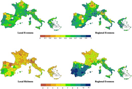
Local and regional agrobiodiversity indices across Mediterranean Europe.
Additional local variables measured by FADN include the percentage of urban land, roads and railroads, ports and airports in the 5-km circle around the farm. We include these measures as proxies for market forces such as market access and the demand for land.
Climate, soil characteristics and population density are also measured for each NUTS3 region. Gridded temperature and precipitation data have been matched with each NUTS3 region from ERA5 dataset (Hersbach et al., 2019). Climate normals are the 30 year (1981–2010) mean values of weather for each NUTS3 region. The seasons are the mean values for the 3 months of each season. For example, the mean of the monthly temperatures of December, January and February are the winter temperatures. Although there is evidence that more spatially refined rainfall measures are more accurate (Fezzi and Bateman, 2015), such data are not available for this sample. The spatial scale of the climate measures could bias the agrobiodiversity coefficients, but the bias is not likely to be large.
Previous studies have included seasonal degree-days as an alternative to temperature. However, there is virtually no difference in the outcomes when using degree-days versus temperature over the growing season (Massetti, Mendelsohn and Chonabayashi, 2016).
Soil data come from topsoil physical properties for Europe (Ballabio, Panagos and Montanarella, 2016) and include percentage of coarse soil, clay soil and bulk soil.
The exact location of each farm is unavailable to us. While FADN used the precise farm locations to measure variables within a 5-km radius, we do not have access to this detailed information. Our only knowledge of each farm’s location is the NUTS3 region in which it is located. As a result, we are unable to test for spatially correlated errors across farms, which may lead to an underestimation of the standard errors in our analysis.
4. Results
The agrobiodiversity results of the Ricardian model of agricultural land value are in Table 3, showcasing estimated coefficients and robust standard errors. Estimates for climate, socio-economic, geographic and soil variables are shown in Table S1 in the Appendix.
Agrobiodiversity coefficients in log-linear regression of farmland value (Euro/ha)
| Coef | SE | |
|---|---|---|
| Local Evenness | 1.012c | 0.103 |
| Local Richness | 0.280c | 0.032 |
| Local Richness_sq | −0.012c | 0.002 |
| Regional Evenness | −4.315c | 0.268 |
| Regional Evenness _sq | 4.793c | 0.254 |
| Regional Richness | 0.368c | 0.046 |
| Regional Richness_sq | −0.016c | 0.003 |
| Interaction Local Evenness & Regional Evenness | −2.073c | 0.176 |
| Interaction Local Richness & Regional Richness | −0.018c | 0.004 |
| Additional controls | Yes | |
| R2 | 0.53 |
Significant coefficients at the 1% level.
SE indicates robust standard errors.
Complete set of coefficients are shown in Table S1 in the Appendix.
Except for local evenness which has a linear effect, the effect of agrobiodiversity is non-linear. The interaction between local and regional agrobiodiversity is consistently characterised by a significant negative coefficient confirming that the two dimensions are linked and substitute for each other. The impact of agrobiodiversity, in general, hinges on the existing level of agrobiodiversity. Farmland values are more sensitive to regional evenness than local evenness. As shown in Figure 2, regional evenness has a convex (U-shaped) relationship with farmland value which implies farmland values are highest when either regional evenness is very low or very high. Some high valued regions specialise in a single high-valued cover type (grains). Other high-valued regions have even distributions of multiple crop types. The regions that have a moderate amount of regional evenness are lower valued. Local evenness is a substitute for regional evenness. More local evenness is beneficial in places with low regional evenness and is harmful in places with high regional evenness. As shown in Figure 3, the effect of richness is concave. There is an optimal amount of regional richness (near 8 to 9 land cover types) and local richness (near 5 to 6 land cover types) in terms of land value. The interaction term is negative, indicating that local richness serves as a substitute for regional richness.
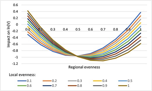
Impact of evenness on farmland value with local–regional interaction.
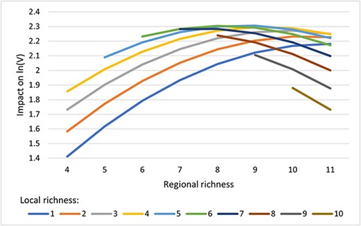
Impact of richness on farmland value with local–regional interaction.
Table 4 details the average marginal impacts of local and regional agrobiodiversity. Increasing local evenness by 10 per cent reduces farmland value by 3.2 per cent, whereas increasing regional evenness by 10 per cent raises it by 5.6 per cent. A 10 per cent rise in local richness increases land values by 2.6 per cent, while the same increase in regional richness boosts farmland values by 3.1 per cent. A simultaneous 10 per cent increase in both local and regional richness and evenness results in an 8 per cent rise in farmland values overall, indicating that moderate, widespread increases in agrobiodiversity can enhance aggregate farmland values.
Marginal impact of agrobiodiversity on farmland value (%/ha)
| Coef | SE | |
|---|---|---|
| Local evenness | −3.16c | 0.003 |
| Local richness | 2.61c | 0.005 |
| Regional evenness | 5. 64c | 0.007 |
| Regional richness | 3.08c | 0.007 |
| Coef | SE | |
|---|---|---|
| Local evenness | −3.16c | 0.003 |
| Local richness | 2.61c | 0.005 |
| Regional evenness | 5. 64c | 0.007 |
| Regional richness | 3.08c | 0.007 |
Significant coefficients at the 1% level.
Marginal impacts are the average of the marginal effect of each variable over all the observations.
Marginal impacts are calculate d for a 1/10 increase in the index.
However, these average effects vary significantly across the southern European landscape. Figure 4 maps the marginal effect of local and regional agrobiodiversity measure across NUTS3 regions, revealing regional disparities in the impacts of increasing agrobiodiversity.
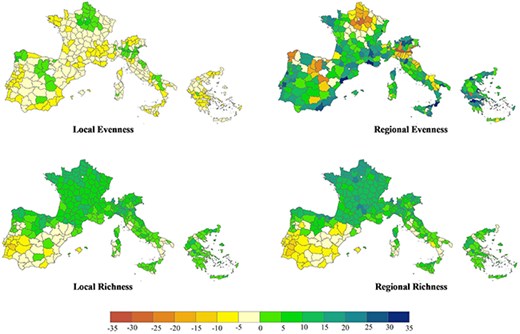
Marginal impacts of agrobiodiversity indices on farmland value (%/ha).
For most regions in southern Europe, increasing regional evenness leads to gains, with farmland values rising by 13 per cent on average, while increasing local evenness results in losses, with an average decline of 4 per cent in farmland values. Conversely, in areas like the northern plains of France, Italy and Spain, which have low regional evenness, increasing regional evenness decreases land values by 11 per cent, while a boost in local evenness can slightly offset this loss, with a 1 per cent gain. This suggests that a universal increase in regional evenness does not guarantee universal benefits, and a universal increase in local evenness is actually harmful on net.
Richness displays a different pattern, as shown in Figure 4. Most of Europe exhibits insufficient richness, and increasing both local and regional richness tends to be beneficial, with farmland values rising by 6 per cent and 9 per cent, respectively, from marginal increases. However, in some regions, largely in southern Spain and Portugal, richness is already at optimal levels and more richness (local or regional) would reduce farmland values by about 4 per cent if either local or regional richness increased.
Table S1 in the Appendix shows the estimated coefficients of the other control variables in the regression. They indicate that higher elevation and larger farmland size reduce farmland value per hectare. Gravelly and sandy soils tend to be harmful, whereas clay soils have a convex impact. Population density and the percentage of urban land (reflecting land scarcity) increase farmland values. Farm subsidies increase farmland value. Land for transport and ports reflect market access and therefore increase farmland value. Both seasonal precipitation and temperature variables are mostly significant, confirming a non-linear response of farmland value to seasonal climate variables. Climate has a very different effect in each season. The squared precipitation coefficients reveal a convex precipitation response in winter and summer and a concave response in autumn and spring. The squared temperature coefficients reveal a convex temperature response in spring and a concave response in autumn, winter and summer. The results align with previous studies examining the impact of climate on farmland values at the European level (e.g. Fabri, Moretti and van Passel, 2022; van Passel, Massetti and Mendelsohn, 2017) and at the country level (e.g. Bozzola et al., 2018).
In Table S2 in the Appendix, we compare the forecasting accuracy of alternative model specifications. Our results confirm that the selected model outperforms alternative specifications.
5. Conclusion and discussion
This study examines the effects of agrobiodiversity on farmland values across five countries in southern Europe, highlighting regional differences in agrobiodiversity levels and their implications. Agrobiodiversity varies widely, with some regions like northern France, Spain and Italy showing low diversity, while others along the Mediterranean coast exhibit much higher levels. These regional differences provide important context for our findings and the broader literature.
We employ a Ricardian model to assess the effects of local and regional agrobiodiversity—measured through evenness and richness—on farmland values, while controlling for critical factors like elevation, soil characteristics, population density, market access and seasonal climate. Our analysis reaffirms that these control variables behave as expected, thereby reducing concerns about omitted variable bias and reinforcing the validity of our model. More importantly, the study isolates the impact of agrobiodiversity on farmland values, which has important economic and ecological implications.
Our findings contribute to the existing literature by underscoring the crucial role that agrobiodiversity plays in promoting the resilience and stability of the agricultural sector. While prior studies have examined the relationship between crop diversity, productivity and risk reduction, this paper adds nuance by emphasising the differential impacts of evenness and richness, across both local and regional scales.
One of the key lessons from this study is the significance of scale in understanding the effects of agrobiodiversity. Regional agrobiodiversity provides resilience against environmental and economic risks, while local agrobiodiversity impacts ecosystem services in ways that may either complement or substitute the benefits of regional biodiversity. The interaction between local and regional agrobiodiversity, consistently characterised by a significant negative coefficient, confirm that these two dimensions are linked and act as substitutes for each other suggesting the importance of accounting for diversity not only within but across landscapes (Concepcion et al., 2012; Tscharntke et al., 2012; Landis, 2017). Moreover, the differential effects of richness and evenness represent an important refinement. Richness has a positive impact at both regional and local scale, though it exhibits diminishing returns. Evenness, a metric rarely examined independently in previous studies, exhibits a U-shaped relationship, where certain regions benefit from the dominance of a few crop types (notably flat plains), while other regions with more varied topographies thrive with a more even distribution of multiple crop types. Our findings also reveal that regional evenness is more impactful than local evenness in most of southern Europe. This supports the argument that larger-scale diversity buffers against environmental and economic risks, providing resilience in agricultural systems. However, in regions like northern France, Spain and Italy, where regional evenness is low, promoting evenness could potentially reduce farmland values.
In comparing our results with previous studies, we find both consistencies and novel insights. Di Falco and Chavas (2008) and Donfouet et al. (2017) emphasised that regional agrobiodiversity acts as a buffer against adverse climatic conditions, especially under water-limited situations, using the Shannon diversity index. Our findings align with these studies in demonstrating that agrobiodiversity, especially at the regional scale, enhances farmland resilience and productivity, reinforcing its economic value. However, our study adds nuance to these conclusions by disaggregating the effects of richness and evenness, as well as examining the non-linear relationships between agrobiodiversity and farmland values, which were not addressed by these earlier studies. Bellora et al. (2018) also observed heterogeneous impacts of crop diversity across landscape scales, with diversity generally showing positive effects but diminishing returns as scale increases. Our results similarly demonstrate that regional diversity positively influences land values, but the magnitude of this effect depends on the existing level of biodiversity and specific local conditions. We extend these insights by highlighting the substitution effect between local and regional biodiversity, suggesting that policy should carefully consider the optimal balance between diversity at different scales. Moreover, Burchfield, Nelson and Spangle (2019) found varying yield responses to different biodiversity metrics, such as richness and the Shannon index, highlighting the importance of separating these effects. Our analysis confirms the importance of distinguishing between richness and evenness, with richness being beneficial in both local and regional contexts, while evenness exhibits more complex, non-linear effects depending on the landscape characteristics. Finally, while previous research has largely concentrated on crop diversity’s role in enhancing productivity (often measured by yield or gross production), our study contributes to the growing body of work recognising the role of agrobiodiversity in supporting ecosystem services that reduce reliance on manufactured inputs. As suggested by Bareille and Dupraz (2020) and Bareille and Letort (2018), biodiversity can lower variable costs by enhancing ecosystem services like pollination, pest control, and soil fertility, leading to higher profitability. Similarly, Auffhammer and Carleton (2018) identified the significance of net revenue as a better measure than yield or gross revenue when assessing the economic value of biodiversity. Our study complements this literature by focusing on farmland values, which implicitly capture both productivity and profitability. By emphasising the non-linear and scale-dependent effects of agrobiodiversity, we contribute to a more nuanced understanding of how biodiversity enhances agricultural resilience and economic value.
From a policy perspective, our findings suggest that biodiversity policies should not adopt a one-size-fits-all approach but rather tailor strategies that consider the interplay between local and regional diversity. In areas with high regional biodiversity, local farmers may be able to specialise more in certain crops, knowing that the broader ecosystem supports them. However, in areas where regional diversity is lower, promoting local diversity becomes essential to resilience.
However, several dimensions of agrobiodiversity remain unexplored in this study. We did not examine which specific crops contribute most to economic resilience, nor did we explore how nearby natural land covers (such as forests or grasslands) might influence farmland values. Additionally, this study focuses solely on the economic value of farmland and does not consider the recreational or aesthetic value of agricultural landscapes, which could also influence land-use decisions in mixed-use areas with residences or tourism. These topics provide fertile ground for future research.
In conclusion, our study confirms the positive role of crop diversity in enhancing agricultural productivity and profitability, while also contributing new insights into the effects of evenness and richness at different scales. Policymakers and practitioners should consider these findings when designing strategies to optimise agricultural systems, particularly in the context of a changing climate where resilience and flexibility are increasingly important. This study adds valuable evidence to the ongoing debate on the role of biodiversity in sustainable agriculture, providing a foundation for more regionally tailored policies that support both economic and environmental goals.
Acknowledgements
Funding was provided by the European Union’s Horizon 2020 research and innovation programme under the Marie Sklodowska-Curie grant agreement No 84215 (CRAS) and the National Recovery and Resilience Plan Mission 4, CUP No E63C22002980006 (BIOA). The authors have no conflicts of interest to declare.
Supplementary data
Supplementary data are available at ERAE online.
