


Abstract
Greater Sage-Grouse (Centrocercus urophasianus) is a species of conservation concern and is highly susceptible to mortality from West Nile virus (WNV). Culex tarsalis, a mosquito species, is the suspected primary vector for transmitting WNV to sage-grouse. We captured, radio-tagged, and monitored female sage-grouse to estimate breeding season (April 15 to September 15) survival, 2016–2017. Deceased sage-grouse were tested for active WNV; live-captured and hunter-harvested sage-grouse were tested for WNV antibody titers. Additionally, we trapped mosquitoes with CO2-baited traps 4 nights per week (542 trap nights) to estimate WNV minimum infection rate (MIR). Eight sage-grouse mortalities occurred during the WNV seasons of 2016 and 2017, 5 had recoverable tissue, and 1 of 5 tested positive for WNV infection. Survival varied temporally with sage-grouse biological seasons, not WNV seasonality. Survival was 0.68 (95% CI: 0.56–0.78; n = 74) during the reproductive season (April 1 to September 15). Mammalian predators were the leading suspected cause of mortality (40%), followed by unknown cause (25%), avian predation (15%), unknown predation (15%), and WNV (5%). These results indicate WNV was not a significant driver of adult sage-grouse survival during this study. Three sage-grouse (1.9%; 95% CI: 0.5–5.9%) contained WNV antibodies. We captured 12,472 mosquitoes of which 3,933 (32%) were C. tarsalis. The estimated WNV MIR of C. tarsalis during 2016 and 2017 was 3.3 and 1.6, respectively. Our results suggest sage-grouse in South Dakota have limited exposure to WNV, and WNV was not a significant source of sage-grouse mortality in South Dakota during 2016 and 2017. Based on our finding that a majority of sage-grouse in South Dakota are susceptible to WNV infection, WNV could potentially have an impact on the population during an epizootic event; however, when WNV is at or near-endemic levels, it appears to have little impact on sage-grouse survival.
Resumen
Centrocercus urophasianus es una especie de preocupación para la conservación y es altamente susceptible a la moralidad causada por el virus del Nilo Occidental (VNO). Culex tarsalis, una especie de mosquito, es el vector primario sospechado de transmitir el VNO a los individuos de C. urophasianus. Capturamos, marcamos con radio y monitoreamos hembras de C. urophasianus para estimar la supervivencia de la estación de cría (15 abril a 15 septiembre) en 2016–2017. Los individuos fallecidos de C. urophasianus fueron testeados para la presencia activa del VNO; los individuos capturados vivos y cazados fueron testeados para la presencia de anticuerpos del VNO. Adicionalmente, atrapamos mosquitos con trampas cebadas con CO2 durante cuatro noches por semana (542 noches de trampa) para estimar la tasa de infección mínima (TIM) del VNO. Ocho muertes de C. urophasianus ocurrieron durante la estación del VNO de 2016 y 2017, cinco tuvieron tejido recuperable, y uno de los cinco dio positivo para la infección del VNO. La supervivencia varió temporalmente con la estación biológica de C. urophasianus, no con la estacionalidad del VNO. La supervivencia fue 0.68 (95% IC: 0.56–0.78; n = 74) durante la estación reproductiva (1 abril a 15 septiembre). Los depredadores mamíferos fueron la principal causa sospechada de mortalidad (40%), seguido de causas desconocidas (25%), depredación por aves (15%), depredación desconocida (15%) y VNO (5%). Estos resultados indican que el VNO no fue un condicionante importante de la supervivencia de los individuos adultos de C. urophasianus durante este estudio. Tres individuos de C. urophasianus (1.9%; 95% IC: 0.5−5.9%) contuvieron anticuerpos del VNO. Capturamos 12,472 mosquitos de los cuales 3,933 (32%) fueron C. tarsalis. La TIM estimada del VNO en C. tarsalis durante 2016 y 2017 fue 3.3 y 1.6, respectivamente. Nuestros resultados sugieren que C. urophasianus en Dakota del Sur tiene una exposición limitada al VNO, y que el VNO no fue una fuente significativa de mortalidad de C. urophasianus en Dakota del Sur durante 2016 y 2017. En base a nuestros hallazgos de que la mayoría de los individuos de C. urophasianus en Dakota del Sur es susceptible a la infección por el VNO, este virus podría potencialmente tener un impacto en la población durante un evento epizoótico; sin embargo, cuando el VNO está en o cerca de niveles endémicos, parece tener poco impacto en la supervivencia de C. urophasianus.
Lay Summary
• West Nile virus is a new disease to the United States. The Greater Sage-Grouse is susceptible to mortality from West Nile virus.
• We captured and radio-tagged sage-grouse to monitor survival. We collected blood from sage-grouse to test for West Nile virus antibodies. We captured and tested Culex tarsalis mosquitoes for West Nile virus. C. tarsalis is a species commonly associated with transmitting West Nile virus.
• Most sage-grouse (70%) died from predation and one of 20 sage-grouse mortalities (5%) was caused by West Nile virus. Overall, we observed low sage-grouse exposure to West Nile virus (<2%). We did not document a decrease in survival during West Nile virus season and found that survival varies with breeding season events for sage-grouse (nesting and brood rearing).
• One caveat is that we found low numbers of mosquitoes carrying West Nile virus, indicating that conditions were not suitable for an outbreak during our study.
INTRODUCTION
Epizootic diseases pose threats to wildlife populations worldwide (Daszak et al. 2000). Zoonotic diseases cycle because of the complex nature of relationships between vectors, hosts, and the environment (Muul 1970, Daszak et al. 2000, Burri et al. 2011). And with the expansion of the human population and anthropogenic effects on landscapes, infectious diseases also have expanded (Daszak et al. 2000, Morse 2001). The cumulative effects of disease with other environmental stressors can significantly increase threats to wildlife populations (Daszak et al. 2003, Pounds et al. 2006, Mills 2012, Taylor et al. 2013).
West Nile virus (WNV) is a zoonotic disease that is relatively new to North America; it was first detected in New York City in the summer of 1999 (Lanciotti et al. 1999). The virus persists in a mosquito–bird–mosquito cycle and has been detected in >300 avian species in the United States (Centers for Disease, Control and Prevention 2015). Greater Sage-Grouse (Centrocercus urophasianus; hereafter sage-grouse) is one avian species that is particularly susceptible to mortality from WNV (Clark et al. 2006). WNV contributed to a 25% decline in survival during an outbreak in 2003 (Naugle et al. 2004); and during a captive study where sage-grouse were experimentally infected with WNV, all sage-grouse died within 6 days of infection (Clark et al. 2006). Sage-grouse infected with WNV exhibit behaviors such as oral/nasal discharge, isolation from group, immobility, drooped wings, labored breathing, and incapability of coordinated locomotion (Clark et al. 2006). These results suggest that WNV-infected sage-grouse might not be able to detect or flee from approaching predators; thus, mortality due to predation may be higher for a WNV-infected sage-grouse.
The first documented sage-grouse mortalities due to WNV occurred in 2003 (Naugle et al. 2004, Moynahan et al. 2006). Shortly thereafter, the first documented sage-grouse to survive a WNV infection were found in the Powder River Basin of Montana and Wyoming in 2005 (Walker et al. 2007). Less than 5% of sage-grouse test positive for WNV antibodies (Walker et al. 2007, Dusek et al. 2014), and it is unknown if WNV antibodies can be passed to sage-grouse chicks from their mothers during egg production via a passive vertical transmission (Walker et al. 2007), as observed in other avian species (Stout et al. 2005, Hahn et al. 2006, Nemeth and Bowen 2007). WNV antibodies have been shown to last at least 5 months in sage-grouse (Walker et al. 2007) and persist for ≥12 months in other avian species (Langevin et al. 2001, Gibbs et al. 2005). It is unknown if or how fast WNV antibodies decrease to undetectable levels in sage-grouse.
Adult female survival has been shown to be a primary population driver for sage-grouse (Johnson and Braun 1999, Sedinger 2007, Dahlgren 2009, Taylor et al. 2012), and other Galliformes as well (Sandercock et al. 2005, McNew et al. 2012). In systems where WNV was likely impacting sage-grouse survival, the lowest seasonal survival occurred during late brood rearing/fall (Wik 2002, Swanson 2009, Blomberg et al. 2013, Davis et al. 2014); however, harvest likely also influenced low fall survival (Wik 2002). Alternatively, other research documented lower survival during nesting and brood rearing during the spring and summer (Connelly et al. 2000a, Moynahan et al. 2006), possibly due to female sage-grouse contending with multiple stressors, both internal (nutritional demands; Dyer et al. 2009) and external (predation; Bergerud and Gratson 1988; Svedarsky 1988).
South Dakota is on the eastern fringe of the current sage-grouse distribution (Schroeder et al. 2004), and WNV has been documented as a source of sage-grouse mortality in the state (Kaczor 2008, Swanson 2009). During annual spring lek counts in 2006, 608 total male sage-grouse were observed, followed by a 44% decline by spring of 2008 (South Dakota Department of Game, Fish and Parks 2014). Additionally, in 2006 and 2007, low adult sage-grouse survival (0.44 and 0.46, respectively) occurred in South Dakota during July‒October (Swanson 2009), and the 2007 annual adult female survival was estimated to be 0.39; this estimate is lower than the range-wide average adult female survival (0.58; Taylor et al. 2012). During this time, WNV was documented as a source of mortality (Kaczor 2008, Swanson 2009), and it is thought that WNV could have caused the population decline. Although only 7% (n = 10) of adult sage-grouse mortalities were confirmed WNV positive during the previous South Dakota study, 17 of 17 sage-grouse tested for WNV in 2006 returned inconclusive test results (Swanson 2009). Additionally, estimated sage-grouse chick mortality attributed to WNV ranged from 6.5% to 71.0% in 2006 and from 20.8% to 62.5% in 2007 (Kaczor 2008). During the 2003 outbreak of WNV in Wyoming, WNV infection was associated with a 25% decline in survival across 4 sage-grouse populations (Naugle et al. 2004). Therefore, WNV has the potential to cause extreme population-level impacts to sage-grouse.
Sage-grouse in South Dakota face unique challenges because they are at the fringe of the species distribution; challenges include increased vulnerability to isolation (Aldridge et al. 2008, Schroeder et al. 2020) and extirpation (Caughley et al. 1988, Lande 1993). When comparing biotic, abiotic, and anthropogenic factors, South Dakota’s occupied sage-grouse range is moderately similar to the extirpated sage-grouse range (Wisdom et al. 2011). This indicates that the South Dakota sage-grouse population may be at risk for extirpation based on habitat and landscape characteristics. WNV in combination with other environmental stressors has been shown to have a more severe additive effect on sage-grouse populations than any factor alone (Taylor et al. 2013). Given South Dakota’s aforementioned risk of sage-grouse extirpation and small population size, the potential additive effects of WNV to sage-grouse mortality could be significant for this particular fringe population.
Culex tarsalis mosquitoes are suspected to be among the most efficient vectors of WNV (Goddard et al. 2002). C. tarsalis primarily obtains blood meals from bird species (Tempelis et al. 1965) and has also been identified as the primary vector of WNV transmission to sage-grouse (Naugle et al. 2004). In the Northern Great Plains, and South Dakota specifically, C. tarsalis is the second most prevalent mosquito (Gerhardt 1966, Easton 1987, Vincent et al. 2020) and is considered the primary vector of WNV (Bell et al. 2005, Johnson et al. 2010, Vincent et al. 2020).
The overall goal of our analysis was to assess the interactions between sage-grouse, C. tarsalis, and WNV in South Dakota. Our specific objectives were to (1) estimate the influence of WNV on sage-grouse survival, (2) document seroprevalence rates of WNV antibodies in sage-grouse, and (3) estimate WNV prevalence rates in C. tarsalis.
METHODS
Study Area
This study primarily occurred in Harding and Butte counties of northwest South Dakota (Figure 1). The land use of the study area is dominated by pastureland (>85%), followed by cropland (10−12%; United States Department of Agriculture 2012); more than 84% of the study area has never been plowed (Bauman et al. 2018). The majority of the land in the study area is privately owned (~75–80%; U.S. Geological Survey, Gap Analysis Program 2016). The monthly average temperature ranges from –1.7 to 10.6°C with an average of 39 cm of precipitation annually (National Oceanic and Atmospheric Administration [NOAA] 2019a). In total, <2% of the study area is open water, woody wetlands, or emergent herbaceous wetlands (United States Geological Survey, National Land Cover Database 2016).
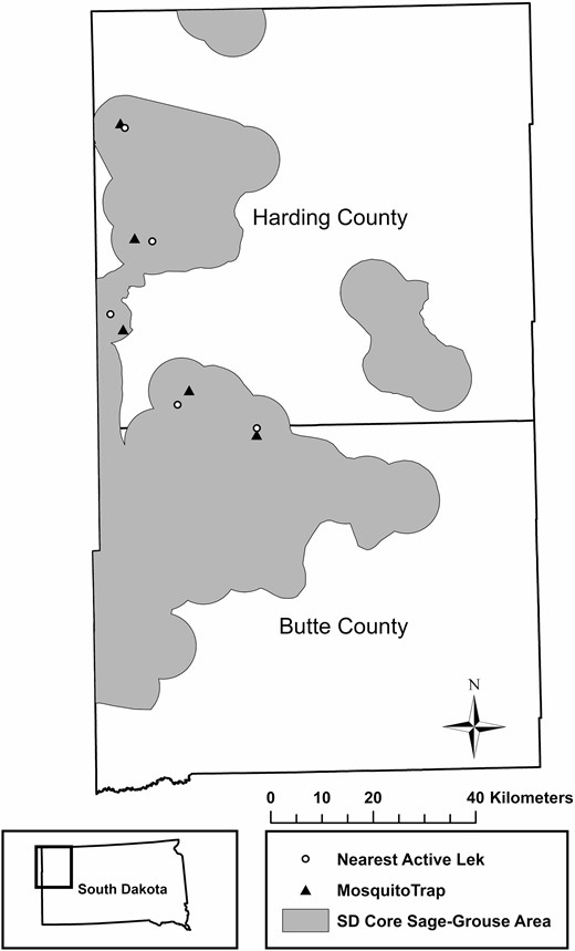
CO2-baited mosquito trap locations and nearest active sage-grouse lek to each mosquito trap. Distance from trap to nearest active lek ranged from 1.3 to 3.8 km.
Our study area represents the eastern edge of the sagebrush distribution where an ecotone between sagebrush steppe and grassland ecosystems occurs (Johnson 1979, Cook and Irwin 1992, Lewis 2004). Sagebrush communities found in South Dakota are shorter and have a lower percent canopy cover than found elsewhere in the sagebrush steppe (Kantrud and Kolgiski 1983, Connelly et al. 2000b, Kaczor et al. 2011). Common shrubs in the study area include silver sagebrush (Artemisia cana) and big sagebrush (Artemisia tridentata; Johnson and Larson 2007).
Sage-Grouse Survival Analysis
We annually captured breeding-age male and female sage-grouse near active leks March–May, as well as at high sage-grouse use areas in August and September using nocturnal spotlighting and a long-handled net (Giesen et al. 1982, Wakkinen et al. 1992). We aged and sexed captured sage-grouse based on plumage and morphological characteristics (Crunden 1963, Beck et al. 1975, Bihrle 1993). We fit female sage-grouse with a 21.6 g necklace-type very high frequency (VHF) radio-tag with an 8-hr mortality switch (model A4060; Advanced Telemetry Systems, Isanti, Minnesota, USA). We weighed all birds at the time of capture to ensure that radio-tags were <3% of body weight (Kenward 2001). Both male and female sage-grouse were fit with a uniquely numbered aluminum butt-end leg band (National Band & Tag Company). All animal handling procedures were approved by the Institutional Animal Care and Use Committee at South Dakota State University (IACUC approval #15-074A).
We monitored VHF signals of all radio-tagged females twice weekly from April 15 to June 14 and daily from June 15 to September 15. Daily monitoring allowed us to reduce bias associated with lag-time in the recovery of corpses in determining true cause-specific mortality (Bumann and Stauffer 2002, Stevens et al. 2011) as well as increase our probability of finding fresh tissue for WNV testing. If a sage-grouse radio-tag signal was detected on mortality mode, the sage-grouse and VHF radio-tag were recovered immediately, and the cause of death was investigated.
We assumed predation occurred if portions of the carcass were consumed. Also, we assumed predation occurred if no carcass could be found, but the collar was removed with evidence of a struggle nearby such as blood on collar or numerous feathers. We differentiated mammalian predation from avian predation based on characteristics found at the mortality site. If bite or chew marks were present on bones or collar, or if the carcass was buried, we assumed mammalian predation (Sargeant et al. 1998). If feathers were plucked, the head was severed, and/or bones and collar did not display chew/bite marks, we assumed avian predation (Grønsdal 2012). We classified it as an unknown source of mortality if there was no apparent blood on collar and we could not locate a carcass or determine a kill site. We also classified it as an unknown source of mortality if a substantial amount of time had passed from the time of death to the time of carcass retrieval, or if the carcass was found intact and did not test positive for WNV.
We used known-fate models in program MARK (White and Burnham 1999) with the logit-link function and staggered entry design (Pollock et al. 1989) to estimate survival. Individuals were considered to have equal survival probabilities regardless of the interval in which they entered the study. We used individual survival status during 7-day intervals for survival modeling. We constructed 2 sets of candidate models. Model set 1 quantified temporal differences in survival among specified seasons (WNV season or breeding season events). Model set 2 quantified the influence of covariates on sage-grouse survival. We used the best approximating model from model set 1 (model with lowest AICc score) as the underlying structure for all models in model set 2 (Burnham and Anderson 2002, Hill et al. 2003, Grovenburg et al. 2012); this method allowed us to first account for seasonal variation in survival, then determine if additional variation could be attributed to individual characteristics (study year or age).
We analyzed sage-grouse survival considering both WNV season impacts and biologically relevant seasons for sage-grouse. We quantified WNV seasonal impacts on sage-grouse survival using 2 different approaches to define the WNV season; both WNV season definitions were informed by mosquito data collected during this study. The first method was the vector-defined infection period, which defined the WNV season beginning and ending with the dates of C. tarsalis detection within our sampling period (June 1 to September 14). This method assumed that if the primary vector was on the landscape, then the potential for WNV existed. We aligned vector-defined WNV season dates with the nearest 7-day interval for survival analysis resulting in June 3 to September 15 being considered the vector-defined WNV season. The second method was a pathogen frequency defined method, which defined the WNV season beginning with the earliest WNV detection in C. tarsalis and ending with the latest WNV detection in C. tarsalis within our sampling period (July 20 to September 14). This method assumed that WNV was not prevalent on the landscape at sufficient frequency to potentially impact sage-grouse prior to our detection of it in the primary vector. We aligned pathogen frequency defined WNV season dates with the nearest 7-day interval for survival analysis resulting in July 22 to September 15 being considered the pathogen frequency defined WNV season.
To facilitate comparison with previous survival analyses in South Dakota, we also used biologically relevant seasons for sage-grouse established by Swanson (2009) with slight modifications. The seasons used in our analysis included pre-nesting (April 1 to April 21), nesting (April 22 to June 9), early brood-rearing (June 10 to July 28), and late brood-rearing (July 29 to September 15). We tested constant survival within each season (.), weekly time-dependent survival (t), and we tested all combinations of adjacent seasons being equal, as well as assessed each season individually while setting the remaining 3 seasons equal to one another. More than 75% of incubation during our study occurred during the specified nesting season. Of all female sage-grouse included in the analysis, 19% had broods at some point during early brood-rearing. We stopped monitoring broods at 7 weeks old; for most this occurred before July 29. Therefore, we could not estimate how many female sage-grouse had broods during the late brood-rearing season. We separated the brood-rearing period into 2 seasons, early and late due to differences in food requirements and behavior during these periods (Peterson 1970, Berry and Eng 1985, Drut et al. 1994, Hannon and Martin 2006). Covariates included in model set 2 were age (adult or yearling) and year (2016 or 2017).
Models were evaluated using Akaike’s Information Criterion corrected for sample size (AICc; Burnham and Anderson 2002). Models within 2 ΔAICc units from the top model were considered candidate models. We included an intercept-only model in both model sets to evaluate relative model fit and explanatory power. An intercept-only model represented constant survival over all 7-day time intervals and no effect of additional covariates.
Although there were different combinations of seasons in each model, as well as a time-dependent model, survival was estimated for each 7-day time interval in all models. We examined our candidate models for uninformative parameters by calculating 85% confidence intervals (CIs) around β parameter estimates; if 85% CI overlapped 0, the variable was deemed uninformative and the model was no longer considered a candidate model (Arnold 2010). If model-selection uncertainty existed, all models within 2 ΔAICc units of the top model were averaged to generate full model-averaged estimates and standard errors (Burnham and Anderson 2002). We did not conduct a goodness-of-fit test because with known-fate data, by definition and design, the saturated model fits the data perfectly (Cooch and White 2016). Reported deviance is the difference in a model’s likelihood from the saturated model and thus provides a measure of relative model fit.
We calculated weekly survival estimates within each season to allow for a standardized comparison of survival among seasons. These were estimated using weighted model averaging of the candidate models; weekly survival estimates were available for each of the 24, 7-day intervals of the study; 95% CIs for the model-averaged weekly estimates were derived using the Delta method. We extrapolated weighted model-averaged weekly survival estimates for the length of each season to estimate survival during each season; 95% CIs were calculated using the Delta method.
WNV Infection in Sage-Grouse
To test for previous WNV infection in sage-grouse, we used a 22-gauge needle to collect 1 mL of blood from the brachial vein (Gregg et al. 2006) of captured sage-grouse. In addition to captured sage-grouse, we opportunistically collected blood from the hearts of harvested sage-grouse during a limited hunting season in 2016. Whole blood was placed in a 2-mL blood tube with a clot activator, then centrifuged within 12 hr of collection. Serum was decanted, frozen, and maintained at −20°C until shipped for testing (Walker et al. 2007). Serum samples were tested for WNV antibodies using a plaque-reduction neutralization assay at Cornell University’s Animal Health Diagnostic Center (Naugle et al. 2004, 2005, Walker et al. 2007). Samples were considered negative for WNV antibodies if titers were not detected at the minimum serum dilution (1:10). Radio-tagged sage-grouse were recaptured at the conclusion of the study. Blood samples were collected and tested for WNV antibodies again; radio-tags were removed. This allowed us to document any radio-tagged sage-grouse that had become infected with WNV, developed antibodies, and survived the duration of the study. The percent of sage-grouse with WNV antibodies was calculated along with symmetrical binomial confidence intervals (95% with 2.5% probability in each tail).
To test for active WNV infection in dead sage-grouse, we recovered any available tissues (intestines, proventriculus, liver, kidney, lung, heart, and brain) from mortalities that occurred from June 1 to September 15. Recovered tissues were frozen until testing for the presence of WNV using a Reverse Transcriptase–PCR Assay at Cornell University’s Animal Health Diagnostic Center (Porter et al. 1993, Shi 2001).
WNV and Vectors on the Landscape
Adult mosquitoes were trapped from June 1 to September 15 using standard miniature light traps with photocell-controlled CO2 release (John W. Hock Company; Model 1012.CO2) 4 nights per week. The CO2 traps were set to deliver 0.5 L CO2 min–1 (Vincent et al. 2020). In South Dakota, it is estimated that 97% of sage-grouse nests are within 7 km of an active lek (Kaczor et al. 2011, Parsons 2019). C. tarsalis have been shown to move >25 km to fulfill life cycle requirements (Bailey et al. 1965); however, most commonly, movements are between 1 and 12.6 km (Milby et al. 1983, Riesen et al. 1992). To study overlapping populations of C. tarsalis and sage-grouse throughout the WNV season, we trapped mosquitoes near active lek sites (within 1.3‒1.8 km of leks; Figure 1). We placed one trap per lek at 5 active leks. Traps were placed in low-level areas that were generally protected from the wind.
Captured mosquitoes were frozen and sorted to species. Female mosquitoes contribute to the transmission of WNV due to their requirement to consume blood meals prior to oviposition (Hubert et al. 1954). Although there are examples of male mosquitoes infected with WNV (Anderson et al. 2006, Unlu et al. 2010), they are typically not of interest when researching WNV (United States Environmental Protection Agency 2017). Therefore, we identified female mosquitoes and sorted each species based on morphological characteristics using a dichotomous identification key (Darsie and Ward 2005). If individual mosquitoes could not be identified due to poor condition, or lacking body parts, we placed them in an “unknown” category.
Several mosquito species known to be found in South Dakota are considered competent vectors of WNV (Woodring et al. 1996, Goddard et al. 2002). However, other than C. tarsalis, all of them primarily feed on mammalian hosts (Tempelis and Washino 1967, Gunstream et al. 1971, Tempelis 1975, Nasci 1984, Anderson and Gallaway 1987, Goudarz and Andreadis 2006) and are less efficient at transmitting WNV than C. tarsalis. Therefore, the other species are likely not a primary vector of WNV to sage-grouse in South Dakota and we opted to test only C. tarsalis mosquitoes for WNV.
Female C. tarsalis were placed in vials of up to 50 individuals, homogenized, and tested for WNV using a TaqMan Reverse Transcriptase–PCR Assay, as described in the work of Lanciotti et al. (2000) with slight modifications. We estimated WNV infection in C. tarsalis using 2 methods. First, we calculated the minimum infection rate (MIR) by counting the number of vials that tested positive divided by a total number of mosquitoes tested times 1,000; MIR is reported as a minimum number of WNV-positive mosquitoes per 1,000 mosquitoes tested. This method assumes the minimum number (one mosquito) is WNV positive in each vial. Second, and similarly, we calculated a prevalence estimate range by assuming either one mosquito in each WNV-positive vial was WNV positive (low end of the range) or that all mosquitoes in each WNV-positive vial were WNV positive (high end of the range), we then divided each of these numbers by all tested mosquitoes resulting in a prevalence range; this number is presented as a percentage of tested C. tarsalis that were WNV positive.
RESULTS
Sage-Grouse Survival Analysis
We monitored 29 and 47 female sage-grouse in 2016 and 2017, respectively. We recorded 11 mortality events each year from April 1 to September 15; however, 2 mortalities occurred within 7 days of capture and, therefore, were censored from further survival analyses (White and Garrott 1990, Kenward 2001). Combining both reproductive seasons, a total of 20 mortality events occurred. Mammalian predation was the leading cause of mortality (40%), followed by unknown sources of mortality (25%), avian predation (15%), unknown predation (15%), and finally, WNV (5%). Predation was the leading cause of mortality of sage-grouse in South Dakota, accounting for ≥70% of breeding season (April 1 to September 15) mortality.
In 2016, 5 of 10 mortalities occurred during the WNV season, 3 of which had sufficient recoverable tissue to be tested for an active WNV infection; none tested positive for WNV. During 2017, 3 of 10 mortalities occurred during the WNV season, 2 of which had recoverable tissue tested for WNV; one tested positive, indicating WNV infection. Overall, we were able to recover sufficient tissue and test 63% (5 of 8) of mortalities for WNV infection.
We included 74 individuals (47 adults and 27 yearlings) in our survival analysis (2016 = 28, 2017 = 46) over a total of 24, 7-day (weekly) intervals. We right-censored individuals that left the study area and were never relocated (n = 6), or if the radio-tag failed (n = 1). Neither of our WNV season models explained more variation in the data than the model of constant survival (Table 1). In our sage-grouse biological timing model set (model set 1), we observed model uncertainty and considered 4 competitive models (<2 ΔAICc units from 0; Table 1). We used the top model as the underlying structure for model set 2 (Table 2). Although within model set 2, models containing the covariates YEAR and AGE were <2 ΔAICc units from 0, the β parameter estimates overlapped 0 (YEAR: β = 0.65, 85% CI: 0.0–1.3; AGE: β = 0.31, 85% CI: –0.36 to 0.97); thus, we deemed the variables YEAR and AGE uninformative and dismissed the models from candidate selection within model set 2. After dismissing models with the addition of YEAR and AGE in model set 2, the only model <2 ΔAICc units from 0 was the top model from model set 1 (Table 2). However, because we experienced model uncertainty within model set 1, we made inferences and calculated survival estimates from the 4 candidate models in model set 1 (Table 1).
Survival models of Greater Sage-Grouse in northwestern South Dakota USA, 2016–2017, from model set 1 evaluating the effects of seasonal timing on survival. Akaike’s Information Criterion corrected for small sample size (AICc; Burnham and Anderson 2002); lowest AICc value = 203.64. ΔAICc is the difference in AICc relative to minimum AICc, wi is Akaike weight (Burnham and Anderson 2002) calculated across all models, and k is the number of parameters.
| Modela | ΔAICc | wi | k | Deviance |
|---|---|---|---|---|
| {Pre(.), Nest(.) = EBR(.) = LBR(.)} | 0.00 | 0.24 | 2 | 199.63 |
| {Pre(.),Nest(.),EBR(.) = LBR(.)} | 0.45 | 0.19 | 3 | 198.08 |
| {Nest(.),Non-Nest(.)} | 1.70 | 0.10 | 2 | 201.34 |
| {Pre(.),Nest(.),EBR(.),LBR(.)} | 1.84 | 0.10 | 4 | 197.45 |
| {Pre(.),Nest(.) = EBR(.),LBR(.)} | 2.01 | 0.09 | 3 | 199.63 |
| {S(.)} | 2.27 | 0.08 | 1 | 203.91 |
| {EBR(.),Non-EBR(.)} | 3.23 | 0.05 | 2 | 202.86 |
| {Non-WNV(vector(.)), WNV(vector(.))} | 3.32 | 0.05 | 2 | 202.95 |
| {Pre(.) = Nest(.),EBR(.) = LBR(.)} | 3.85 | 0.03 | 2 | 203.48 |
| {Non-WNV(fqcy(.)), WNV(fqcy(.))} | 4.15 | 0.03 | 2 | 203.78 |
| {Pre(.) = Nest(.) = EBR(.),LBR(.)} | 4.19 | 0.03 | 2 | 203.83 |
| {Pre(.) = Nest(.),EBR(.),LBR(.)} | 5.23 | 0.02 | 3 | 202.85 |
| {S(t)} | 26.32 | 0.00 | 24 | 180.95 |
a Pre = pre-nesting season (April 1–21), Nest = nesting season (April 22 to June 9), EBR = early brood-rearing season (June 10 to July 28), LBR = late brood-rearing season (July 29 to September 15), Non-nest = pre-nesting, early brood rearing, and late brood rearing, Non-EBR = pre-nesting, nesting, and late brood rearing, Non-WNV(vector) = not considered WNV season using vector presence to define (April 1 to June 2), WNV(vector) = WNV season using vector presence to define (June 3 to September 15), Non-WNV(fqcy) = not considered WNV season using pathogen frequency to define (April 1 to July 21), WNV(fqcy) = WNV season using pathogen frequency to define (July 22 to September 15), (.) = constant survival, “=” seasons were set equal to one another.
Survival models of Greater Sage-Grouse in northwestern South Dakota and USA, 2016–2017, from model set 2 evaluating effects of the year (2016 or 2017) and age (juvenile or adult) on survival. Akaike’s Information Criterion corrected for small sample size (AICc; Burnham and Anderson 2002); lowest AICc value = 203.62. ΔAICc is the difference in AICc relative to minimum AICc, wi is Akaike weight (Burnham and Anderson 2002) calculated across all models, and k is the number of parameters.
| Modela | ΔAICc | wi | k | Deviance |
|---|---|---|---|---|
| {S(Pre(.), Nest(.) = EBR(.)+LBR(.) + YEAR} | 0.00 | 0.32 | 3 | 197.60 |
| {Pre(.), Nest(.) = EBR(.) = LBR(.)} | 0.02 | 0.32 | 2 | 199.63 |
| {S(Pre(.), Nest(.) = EBR(.) = LBR(.) + AGE} | 1.60 | 0.14 | 3 | 199.20 |
| {S(Pre(.), Nest(.) = EBR(.)+LBR(.) + YEAR + AGE} | 2.01 | 0.12 | 4 | 197.60 |
| {S(.)} | 2.29 | 0.10 | 1 | 203.91 |
| {S(t)} | 26.33 | 0.00 | 24 | 180.95 |
| {S(t + YEAR + AGE)} | 28.56 | 0.00 | 26 | 179.00 |
a Pre = pre-nesting season (April 1–21), Nest = nesting season (April 22 to June 9), EBR = early brood-rearing season (June 10 to July 28), LBR = late brood-rearing season (July 29 to September 15), Non-nest = pre-nesting, early brood rearing, and late brood rearing, Non-EBR = Pre-nesting, nesting, and late brood rearing, YEAR = study year, 2016 or 2017, AGE = juvenile or adult, (.) = constant survival, “=” seasons were set equal to one another.
All 4 models indicated the highest survival during pre-nesting. We observed no mortality events during the 3-week pre-nesting season that resulted in inflated error estimates. However, because of the necessity to estimate survival during each 7-day interval, we retained all 4 models as candidate models. Using model-averaged estimates of the 4 candidate models’ real function parameter estimates (parameter estimates that are presented on the probability scale) for each season, we estimated survival at 0.68 (95% CI: 0.56–0.78) for April 1 to September 15.
Weighted model-averaged weekly survival estimates during each season were pre-nesting = 1.0 (95% CI: 0.99–1.0), nesting 0.98 (95% CI: 0.96–0.99), early brood rearing = 0.98 (95% CI: 0.97–0.99), and late brood rearing 0.98 (95% CI: 0.97–0.99). We estimated survival for each season by extrapolating model-averaged weekly survival estimates to the length of each season. Estimated survival from the beginning to the end of the 3-week pre-nesting season was 0.99 (95% CI: 0.97–1.00; 3 weeks). The remaining seasons were 7 weeks long; estimated survival from the beginning to the end of the nesting season was 0.85 (95% CI: 0.76–0.94), early brood-rearing season was 0.90 (95% CI: 0.83–0.97), and late brood-rearing season was 0.89 (95% CI: 0.83–0.96; Figure 2).
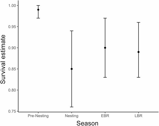
Model-averaged survival estimates for each season within the annual reproductive period. Error bars represent 95% confidence intervals. Pre-nesting (April 1–21; 3 weeks), nesting (April 22 to June 9; 7 weeks), early brood rearing (EBR; June 10 to July 28; 7 weeks), and late brood rearing (LBR; July 29 to September 15; 7 weeks). West Nile virus was detected in Culex tarsalis as early as July 20 and as late as September 14. West Nile virus season completely overlaps with late brood-rearing season and partially overlaps with early brood-rearing season.
WNV Infection in Sage-Grouse
We tested 158 individual sage-grouse that were either live-captured or hunter-harvested (76 females and 82 males) for WNV antibodies; 3 sage-grouse (1.9%; 95% CI: 0.4%–5.5%) contained WNV antibodies, 2 females (2.6%; 95% CI: 0.3%–9.1%) and 1 male (1.2%; 95% CI: 0.03%–6.6%). In total, we recaptured 17 radio-tagged female sage-grouse at the conclusion of the study (44% of remaining radio-tagged sage-grouse) to remove collars and collect blood samples. No sage-grouse had developed WNV antibodies since their original capture; however, 1 individual positive for WNV antibodies at initial capture still contained detectable levels of WNV antibodies upon recapture (199 days between captures; ≥1 year post-WNV infection). This individual was initially captured in early spring and WNV antibodies were detected. Mosquitoes are not active in South Dakota in early spring; thus, the antibodies were assumed to be from a WNV infection during a previous WNV season (≥6 months prior). The second capture of this individual occurred 199 days after the first capture and the individual still contained detectable levels of WNV antibodies. If we assume the antibodies were from a single, previous WNV infection, then by default, the antibodies had been present for >1 year post-WNV infection. Two other individuals contained detectable levels of WNV antibodies upon initial capture but were not recaptured at the conclusion of the study; the female sage-grouse died during the study and because male sage-grouse only received a leg band, we were unable to track and recapture it, thus, this individual’s fate was unknown.
WNV and Vectors on the Landscape
We collected a total of 12,472 mosquitoes over 542 trap nights, 32% of which were C. tarsalis (Table 3). A total of 12 mosquito species were identified; but C. tarsalis, Aedes vexans, Aedes dorsalis, and Culiseta inornata accounted for over 94% of the total number sampled (Table 3). In 2016, 6 WNV detections occurred at 4 of 5 CO2 mosquito trap sites. In 2017, there were 3 WNV detections, occurring at 2 of 5 CO2 mosquito trap sites. When standardized by trap night, there were more total mosquitoes and C. tarsalis captured per trap night in 2016 (26.1 and 7.6, respectively) than in 2017 (20.3 and 7.0, respectively). Estimated WNV MIR of C. tarsalis ranged from 1.6 to 3.3 (Table 3). Estimated WNV prevalence in C. tarsalis during our study ranged from 0.2% to 7.8% (Table 3). In 2016 and 2017, 3.3% and 1.5%, respectively, of mosquito pools (vials) tested positive for WNV.
Total numbers of mosquitoes collected from June 1 to September 15, 2016 and 2017 using 5 CO2 traps in Butte and Harding counties, South Dakota. West Nile Virus (WNV) detections occurred between July 20, 2016 and September 4, 2016 and between July 27, 2017 and August 23, 2017.
| 2016 | 2017 | Total | |
|---|---|---|---|
| Trap nights | 252 | 290 | 542 |
| WNV minimum infection rate | 3.3 | 1.6 | 1.6–3.3 |
| Estimated WNV prevalence (%) | 0.3–7.8 | 0.2–4.9 | 0.2–7.8 |
| Culex tarsalis | 1,915 | 2,018 | 3,933 |
| Ochlerotatus dorsalis | 1,627 | 1,776 | 3,403 |
| Aedes vexans | 1,241 | 871 | 2,112 |
| Culeseta inornata | 1,557 | 747 | 2,304 |
| Other or unknown | 233 | 487 | 720 |
| Total | 6,573 | 5,899 | 12,472 |
DISCUSSION
We found that WNV did not have a significant impact on sage-grouse survival. Survival models that included the effects of WNV did not perform significantly better than constant survival models; if WNV was significantly impacting sage-grouse survival, we would expect to see lower survival during the WNV season, which we did not. We observed one mortality attributed to WNV during both breeding seasons; nearly all other mortalities were due to predation. Although we assume WNV-infected sage-grouse were more susceptible to predation, we did not observe an overall increase in mortality during the WNV season. Based on these observations, we conclude that WNV was not a significant source of mortality for sage-grouse during our study. Moreover, we found that sage-grouse survival varied with biological seasons more than WNV season.
When we compare our survival estimates during WNV season to those reported in the literature, we find that our survival estimates overlap with survival estimates from populations known to have experienced a WNV outbreak as well as those unaffected by WNV. For example, Naugle et al. (2004), Walker et al. (2004), and Moynahan et al. (2006) each reported survival estimates for late summer (July 1 to August 31) as 0.64, 0.20, and 0.84, respectively, for WNV-affected populations and reported survival estimates of 0.76 (Walker et al. 2004) and 0.89 (Naugle et al. 2004) for populations unaffected by WNV. Our derived survival estimate (extrapolated using model-averaged weekly survival rates) for the same time period was 0.87 (95% CI: 0.79–0.94), which appears to better align with the non-WNV-affected populations. Alternatively, Naugle et al. (2005) compared survival rates from 12 different study sites experiencing different WNV scenarios and found that survival rates from July 1 to mid/late September in WNV-affected populations ranged from 0.83 to 0.92, whereas the unaffected populations’ survival rates ranged from 0.92 to 1.0. Our survival estimate extrapolated for this time period was 0.84 (95% CI: 0.75–0.93), which aligns with the WNV-affected populations’ survival estimates reported by Naugle et al. (2005). These comparisons emphasize the variability in sage-grouse survival relative to the severity of a WNV outbreak, but also in the absence of WNV.
We also found limited evidence that sage-grouse can develop and maintain WNV antibodies. We observed a low occurrence of sage-grouse with WNV antibodies (1.9%), which was consistent with previous research (Walker et al. 2007, Dusek et al. 2014), and indicated that it is possible for sage-grouse in South Dakota to survive WNV infection. The low occurrence of antibodies suggests 4 non-mutually exclusive possibilities: (1) that the majority of sage-grouse have not been exposed to WNV and, therefore, have had no opportunity to develop antibodies; (2) that WNV is lethal to the majority of the population and that there are a limited number of birds with the ability to survive the infection and develop antibodies; (3) that WNV antibodies in sage-grouse wane through time to undetectable levels and, therefore, we could not detect the previous infection after a given amount of time; or (4) that sage-grouse are mounting an immune response other than via producing WNV-specific antibodies (e.g., innate or antigen nonspecific immune response) and, thus, we cannot detect the previous infection by evaluating WNV antibodies. The fourth possibility was observed in a budgerigar (Melopsittacus undulates) that was indeed harboring WNV infection within the heart tissue but showed low viremia levels (only detected day 1 post-inoculation) and did not develop WNV antibodies over the course of the study (14 days; Komar et al. 2003). Walker and Naugle (2011) predicted sage-grouse resistance to WNV would only marginally increase over a 20-year period and resistance would remain relatively low; our finding of low numbers of WNV-exposed individuals supports this prediction.
We documented detectable WNV antibodies in sage-grouse ≥12 months post-infection, which is longer than previously documented (<6 months) for sage-grouse (Walker et al. 2007). Although it is possible that this individual became re-infected with WNV between sampling periods, this is unlikely based on the low levels of WNV detected on the landscape during the study.
One caveat to our findings includes our overall low (0.2–7.8%) WNV prevalence in mosquitoes. Our conclusion that WNV was not a significant source of mortality for sage-grouse during our study is contingent on the fact that we did not observe a high prevalence of WNV in mosquitoes; our conclusion may be different under scenarios where WNV prevalence in mosquitoes is higher. Although our range of WNV prevalence in mosquitoes was 0.2–7.8%, the true prevalence rate was likely at the low end of this range because mosquitoes were tested in vials of up to 50 mosquitoes. Each positive result could be 1 in 50 mosquitoes was positive for WNV or 50 of 50 mosquitoes were positive for WNV. However, a majority of the vials contained no WNV-positive mosquitoes; therefore, we suspect that 50 of 50 (or other high rates) mosquitoes testing positive for WNV is unlikely.
The MIR documented in the sagebrush steppe in Wyoming during an outbreak year was 7.16, this outbreak was suspected of causing a 25% decline in that study’s sage-grouse population (Naugle et al. 2004); their reported MIR was higher than in our study (1.6–3.3). In the sagebrush steppe in Alberta, mosquitoes were sampled during a WNV outbreak year and a non-outbreak year. During the outbreak year, 12.2% of mosquito vials tested positive, while the non-outbreak year had <1% of mosquito vials test positive (Naugle et al. 2005). Our study found 3.3% and 1.5% of vials tested positive for WNV in 2016 and 2017, respectively. It appears that the WNV prevalence in C. tarsalis documented during our study was lower than documented in other states and provinces during WNV outbreak years, while slightly higher than the reported non-outbreak year.
Our finding of low WNV prevalence in mosquitoes during this study could be due to environmental factors such as precipitation and temperature, which have been shown to affect C. tarsalis development and WNV transmission rates (Hagstrum and Workman 1971, Hubálek and Halouzka 1999, Epstein 2001, Reisen et al. 2006, Ruiz et al. 2010, Chuang et al. 2011, Danforth 2015). Specifically, in the Northern Great Plains region, higher temperatures and higher precipitation had positive influences on C. tarsalis abundance (Chuang et al. 2011). However, when we compared weather trends during our study to previous research in South Dakota (2006–2007) where WNV outbreaks occurred (Kaczor 2008, Swanson 2009), we did not detect patterns differentiating previous outbreak years (2006 and 2007) from non-outbreak years (2016 and 2017). When comparing monthly weather data (Palmer Drought Severity Index, maximum temperature, minimum temperature, average temperature, and total precipitation) from June to September 2006, 2007, 2016, and 2017, values often overlapped with no clear separation between study years in any single metric.
There is some evidence that drought can contribute to the severity of WNV (Paull et al. 2017), and although July and August 2006 were the 8th driest on record for the study area (1895–2019; NOAA 2019b), we found similar dry conditions during our study, with July 2017 being the 14th driest on record (NOAA 2019b). It is possible that specific timing of weather events within each month was significant yet not detected at a monthly scale, or a combination of factors contributed to creating conditions suitable for a WNV outbreak in 2006 and 2007.
We estimated a low prevalence of WNV in C. tarsalis, which mirrors the low prevalence of WNV in sage-grouse. This suggests that the transmission rate of WNV is reflective of the number of vector encounters, as well as the proportion of infected vectors (Thrall et al. 1993, 1995). We do not have a relative index of C. tarsalis abundance for the study area over time to determine whether the numbers observed were above, below, or average for the area. However, in a year with environmental conditions favorable for C. tarsalis (higher temperatures and higher precipitation; Chuang et al. 2011), we would expect higher numbers of C. tarsalis and higher numbers of vector encounters. Thus, in a year with favorable conditions, we may expect a WNV epizootic event.
Moreover, sage-grouse in South Dakota are already vulnerable to isolation and extirpation and have experienced population declines potentially linked to prior WNV outbreaks. Therefore, if a WNV outbreak occurred, and if sage-grouse in South Dakota experienced decreased survival because of WNV, then the risk of extirpation for this vulnerable population may be exacerbated. Although there is considerable fluctuation in WNV prevalence across years, even in low WNV incidence years, the virus persists at a baseline or endemic level on the landscape (Lindsey et al. 2010). The WNV levels documented in our study may reflect baseline or endemic levels for northwest South Dakota. Based on our finding that a majority of sage-grouse in South Dakota are susceptible to WNV infection, WNV could potentially have an impact on the population during an epizootic event; however, when WNV is at or near-endemic levels, it appears to have little impact on sage-grouse survival.
ACKNOWLEDGMENTS
We thank the private landowners who granted us access to their land to conduct this research. We appreciate the South Dakota Department of Health, and C. Carlson, for testing our mosquitoes for West Nile virus. We thank C. Berdan and E. L. Mitchell for assiting with sage-grouse capture. We also sincerely thank J. M. Gehrt, C. E. Sink, K. A. Norton, S. C. Arent, R. Alley, and D. Pecenka for collecting and sorting mosquitoes and monitoring sage-grouse survival.
Funding statement: Funding for this work was provided by South Dakota Game, Fish, and Parks, State Wildlife grant T-70-R-1 #2481. This publication was also supported by a grant from the National Aeronautics and Space Administration Applied Sciences Health and Air Quality Program (grant No. NNX15AF74G).
Ethics statement: This research was conducted in compliance with the Guidelines to the Use of Wild Birds in Research. All animal handling procedures were approved by the Institutional Animal Care and Use Committee at South Dakota State University (IACUC approval # 15-074A). We used South Dakota Collection Permit #12.
Author contributions: The idea, design, and experiment were conceived by J.A.J., T.J.R., and G.P.V. The research was supervised by J.A.J. and A.J.G. Data were collected and experiments were performed by L.A.P. and T.J.R. The paper was written by L.A.P. with substantial edits from A.J.G., J.A.J., and T.J.R. Methods were developed and designed by L.A.P., G.P.V., T.J.R., J.A.J., and A.J.G. The data were analyzed by L.A.P.
Data availability: Analyses reported in this article can be reproduced using the data provided by Parsons et al. (2021).
