


Abstract
An understanding of how tropical bird communities might respond to climate change and other types of environmental stressors seems particularly urgent, yet we still lack, except for a few sites, even snapshot inventories of avian richness and abundances across most of the tropics. Such benchmark measurements of tropical bird species richness and abundances could provide opportunities for future repeat surveys and, therefore, strong insight into degrees and pace of change in community organization over time. The challenges of creating a network of benchmarked sites include high variation in detectability among species, general rarity of many species that creates hurdles for use of modern bird counting methods aimed at controlling for variation in detectability, and lack of a standardized protocol to create repeatable inventories. We argue that reasonably complete inventories of tropical bird communities require use of multiple survey techniques to provide internal calibrations of abundance estimates and require multiple visits to improve completeness of richness inventories. We suggest that a network of large (50–100 ha) plots scattered across the tropics can also provide insights into geographic variation in and drivers of avian community structure analogous to insights provided by the Smithsonian Center for Tropical Forest Science Forest Global Earth Observatory network of forest dynamics plots. Perhaps most importantly, large plots provide opportunities for use of multiple survey techniques to estimate abundances while also using some exactly repeatable survey techniques that can greatly improve abilities to quantify change over time. We provide guidance on establishment of and survey methods for large tropical bird plots as well as important recommendations for collection and archiving of metadata to safeguard the long-term utility of valuable benchmark data.
Resumen
Entender cómo las comunidades de aves tropicales podrían responder al cambio climático y otros tipos de estresores ambientales parece particularmente urgente; sin embargo, con excepción de algunos pocos sitios, aún nos faltan inventarios incluso acotados de riqueza y abundancia de aves para la mayor parte de los trópicos. Tales mediciones de referencia de riqueza y abundancia de especies de aves tropicales podrían permitir muestreos repetidos a futuro y, por ende, brindarnos una acabada comprensión del grado y ritmo de cambio en la organización comunitaria a lo largo del tiempo. Los desafíos de crear una red de sitios de referencia incluyen alta variación en detectabilidad entre especies, rareza general de muchas especies lo que representa un obstáculo para el uso de métodos modernos de conteo de aves dirigidos a controlar la variación en detectabilidad, y falta de un protocolo estandarizado para obtener inventarios repetibles. Argumentamos que los inventarios razonablemente completos de comunidades de aves tropicales requieren el uso de múltiples técnicas de muestreo para brindar calibraciones internas de estimaciones de abundancia, y múltiples visitas para mejorar la integridad de los inventarios de riqueza. Sugerimos que una red de parcelas grandes (50–100 ha) distribuidas a través de los trópicos puede brindar información de la variación geográfica y los responsables de la estructura de las comunidades de aves, análoga a la información brindada por la red de parcelas de dinámica de bosque del Centro Smithsonian para Ciencia Forestal Tropical-Observatorio Mundial de Tierras Forestales (CTFS-ForestGEO). Quizás lo más importante es que las parcelas grandes brindan oportunidades para el uso de múltiples técnicas de muestreo para estimar las abundancias y al mismo tiempo utilizan algunas técnicas de muestreo exactamente repetibles que pueden mejorar en gran medida las habilidades para cuantificar cambios en el tiempo. Brindamos orientación sobre el establecimiento y los métodos de muestreo para parcelas grandes de aves tropicales, así como recomendaciones importantes de colecta y archivado de meta-datos para salvaguardar la utilidad a largo plazo de datos de referencia valiosos.
INTRODUCTION
Birds play important ecological roles, for example, as predators of herbivorous arthropods and as long-distance dispersers of seeds (Sekercioglu 2006). Birds also pollinate plants and are likely to move pollen long distances (Bawa 1990, Volpe et al. 2014). Many plant species are specialized to interact with birds. In the Neotropics, for example, the majority of tree species use frugivorous birds for seed dispersal (Howe and Smallwood 1982). Yet, unlike extensively studied tropical tree communities (Condit 1995, Condit et al. 2005, Feeley and Silman 2011), in-depth local studies of tropical bird communities characterizing richness and abundance sufficient to address questions of broad ecological relevance lag far behind. The lag is no doubt influenced by the difficulties of detecting tropical birds (Robinson et al. 2019). Many species may be silent or vocalize rarely, are obscured from sight by dense vegetation, difficult to hear because of high-pitched sounds uttered from high canopy locations, or so mobile that certainty about degree of use of sites where the birds are detected is problematic. Nevertheless, birds are prominent occupants of tropical habitats, play key roles in interactions with plants and other animal species, and should be monitored with systematic protocols given our lack of detailed knowledge about many tropical bird communities and their responses to accelerating global change.
Numerous basic scientific questions can be addressed with standardized bird data from large plots. For example, what is the relationship between avian and tree species richness across geographic locations? How does the abundance of avian insectivores vary with respect to tree species diversity and environmental characteristics (e.g., seasonality, rainfall, latitude)? How does the estimated annual consumption of fruit and arthropods by birds relate to the diversity of seed dispersal strategies by trees and leaf renewal rates or diversity of chemical defense mechanisms? How does the trophic structure of bird communities vary across geography? These are just a few examples of the ecological questions that could be addressed if bird community data were available to link directly with plant community data such as those gathered on large forest dynamics plots.
Beyond an opportunity to address ecological questions of broad interest, data on tropical bird communities are important in this era of dynamic environmental change. Despite tropical habitats being home to the majority of bird species, comparatively few data exist to document the current richness and abundance of their bird communities. The shortage of data impedes our ability to understand how tropical bird communities are changing or will change as climatic variables fluctuate over time, as humans influence the structure of surrounding landscapes, and as populations of migratory birds that spend parts of each year in the tropics are influenced by factors far away. The most rigorous way to quantify change would involve exactly repeating community-level surveys at sites with pre-existing benchmark community surveys.
We define benchmarks as community-level surveys establishing reference measurements of richness and abundance against which all future surveys can be compared because at least some of the methodology used is exactly repeatable. Tropical bird community benchmarks are rare. Although there has been longstanding interest in the structure of tropical bird communities (Karr 1976, Terborgh et al. 1990, Thiollay 1994, Robinson et al. 2000, Johnson et al. 2011, Blake and Loiselle 2016), the methods used to quantify abundances and community structure have varied across studies and suffered from poor or non-existent archiving of metadata. Without specific details of the methodology utilized to establish survey locations, count birds, and analyze count data, repeating surveys in statistically meaningful ways becomes a serious challenge.
Many investigators have identified the need for large plots (approaching or exceeding 100 ha in forests) if a majority of bird species in tropical forest communities (typically species-rich and difficult to survey compared with many other habitat types) are to occur at sufficiently high abundances to enable enumeration (Terborgh et al. 1990, Robinson et al. 2000). A tradeoff occurs, of course, where the time and resources needed to establish and survey large areas are balanced against the information gained. We suggest that a key value of large plots has been largely overlooked, the benchmarking value. By incorporating into the survey methodology some portion of effort that is exactly repeatable, with attention paid to preserving essential metadata properly, future surveys can influence our understanding of community change over time, even if each plot survey event might result in an overall incomplete assessment of all species’ abundances within the community.
Here, we outline a survey protocol to collect data on the presence and abundance of birds in and around large (50 ha and larger) plots in a standardized manner. We focus on large plots in forests because (1) several existing large plots (e.g., Cocha Cashu, Peru; Limbo, Panama) have been established across the Neotropics, thus providing a network of sites with which comparisons of data from new plots can be facilitated; (2) information on bird community structure could be linked with tropical tree community structure because of the extensive Center for Tropical Forest Science Forest Global Earth Observatory (CTFS-ForestGEO) network of tropical plots; (3) large plots can be placed in landscapes of perceived particular conservation relevance and enhance the value of those sites for protection; and (4) the greater effort required to sufficiently inventory large plots may have a stronger chance of more fully characterizing local bird communities than rapid, yet easily accomplished, road- or trail-side surveys.
Historically, surveys of large tropical plots relied heavily on spot-mapping. Our protocol combines multiple survey methods to generate data for estimating species richness and abundances of terrestrial birds in plots regardless of geographic location. A primary driving force for incorporation of multiple methods is to provide multiple approaches for adjusting abundance estimates based on detectability factors. Even with multiple approaches, however, estimates of abundance for some elusive species probably can only be achieved by observers who have invested sufficient time on a plot to understand the bird community well. Tropical bird communities, with the ubiquitous long tail of rare species, continue to pose challenges for data-hungry analytical methods, but new approaches continue to be developed. Survey design considerations, emphasizing repeatability of methods, can circumvent limitations of current analytical techniques (Banks-Leite et al. 2014).
METHODS
Survey Methods
Given our recommendations for plot-based surveys, it might be ideal to set as a goal the estimation of population density for each species. Yet, because many birds may move on and off study plots, covering areas of unknown size, we use the term abundances instead. The protocol utilizes combinations of established survey methods to estimate abundances of birds: (1) line-transect surveys with distance estimation, and (2) point-transect surveys with distance estimation and time-of-detection recorded. The line-transect method involves counting all birds along a pre-defined transect (Järvinen and Väisänen 1975), whereas the point-transect method involves counting birds at pre-defined points along a transect (Buckland 2006). Distance-sampling methods involve recording the distances of detected birds from a line or point, allowing the practitioner to estimate distance-based detection probabilities to correct raw count data such that abundance can be estimated (Buckland et al. 2007). The time-of-detection method involves dividing counts into several time intervals and recording detections of individual birds in each interval (Alldredge et al. 2007), which allows estimation of species-specific probability of detection.
With distance sampling, we can estimate abundances from the observations, using the software program DISTANCE (http://www.ruwpa.st-and.ac.uk/distance/). Inputs required are, for each observation: location of the observer on the plot, and direction and distance to the observed bird(s). Direction is necessary because the software calculates perpendicular distance of the bird from the transect, not from the observer. Modified versions of the calculations are used when estimating abundance from points so that the distances from the observer at a point to birds are included. Noting direction from points is important as well because the locations of the birds can be used later to spot-map and identify clusters of locations denoting potential territorial boundaries for species that utilize such space-use strategies.
This combination of line transects with distance estimation, point counts with distance estimation, and point counts with time intervals will provide 3 ways to adjust abundance estimates for variation in detectability. A fourth abundance estimate will come from mapping the locations of all birds detected during transect surveys and point counts. Since direction and distance of each bird from the observer is noted, we then use those data to map occurrences of each species. Interpretation of the spot maps will be best performed by the observers who collected the data because those observers will know how to evaluate whether or not certain clusters of birds were likely to be different birds or the same birds moving around the plots.
Survey Area
No one has yet rigorously studied the optimal size of tropical bird plots in any habitat. Most past studies of forest plots have surveyed 100 ha because that size seems to balance the effort required to survey the plot against the loss of information on a few species that utilize much larger areas (e.g., raptors, some parrots, some wide-ranging groups such as hummingbirds and ant-following birds). We recommend the survey area should minimally amount to 49 ha of mapped habitat so that the entire surveyed area including a buffer around the 49 ha approaches 100 ha. The size of 49 ha mapped and transected relates to the existing design of many CTFS ForestGEO plots. Some of those plots are rectangular and measure 500 × 1,000 m, giving a total of 50 ha, whereas others are 700 × 700 m, totaling 49 ha. Our recommendations below are based on rectangular 50-ha plots but practitioners may need to adjust to local circumstances, such as topography that may influence the exact shape of plots (Figure 1).
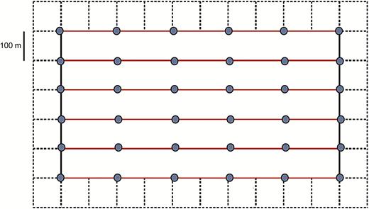
Design of line transects and point count distribution for bird surveys on benchmarking plots. Depicted is a typical 500 m (north–south) by 1,000 m (east–west) gridded plot. Each of 6 line transects 1 km in length (red lines) are walked and surveyed following the line-transect survey protocol. Along those line transects, observers stop every 200 m (gray circles) and conduct an 8-min point count following the point count survey protocol. When birds detected up to 100 m away from the plot are included in surveys, the total area sampled is 84 ha (dashed lines around periphery of core 50-ha plot). When effective detection distances exceed 100 m, the sampled plot size increases accordingly.
The effective survey area will be larger, as surveys conducted along the boundaries of the survey area will include birds detected outside the plots, up to at least 100 m away. Thus, for a rectangular 50-ha plot (Figure 1), the area effectively surveyed is ~84 ha, which approaches the 100-ha size used in several previous studies of Neotropical bird communities (Terborgh et al. 1990, Robinson et al. 2000). For a square 49-ha survey area, the effective area surveyed is ~81 ha. For species that can be detected with confidence at greater distances, the surveyed plot size increases accordingly, and decreases for species with lower detection distances. When calculating the estimated abundance of a species on the plot, it is important to document how far outside the mapped and transected portion of the plot each species was detected and report the “effective” plot size for each species.
Spatial Layout
Across the entire length of the survey area, line transects are established at an interspacing of 100 m. That distance was selected to increase the likelihood of detecting species that do not vocalize much but may be difficult to see in densely vegetated plots, and of species whose vocalizations do not carry more than 50 m.
Along these line transects, stationary (point) count stations are established every 200 m as a way to generate another estimate of abundance without slowing progress along the walking transects too much during a morning’s survey. We do suggest combining transect walks and stationary counts during each morning of survey effort, an approach we explain in more detail later. The spatial layout for a survey area of 500 × 1,000 m (50 ha) is shown in Figure 1. Total transect length thus amounts to 7,000 m for a 500 × 1,000 m plot (6 transects of 1,000 m + 2 sides of 500 m). The associated number of points will be 36.
This layout can be modified to fit any plot size following these basic rules: (1) line transects should be located every 100 m across the plot in a parallel arrangement with the longer side of plots, and (2) point count locations should be located at 200-m intervals along the transects. By following this protocol, comparisons are possible even across sites that have different-sized plots.
Observers
Surveys of birds should be done by 2 or 3 experienced observers if possible. Plots can be surveyed by highly experienced individual observers, but opportunities to compare among observers are then lost. The observers should know all songs and calls and be able to identify by sight all species expected to occur in the area. Observers can survey different parts of the plot simultaneously. In cases where one observer is training another observer, the 2 can conduct surveys together. Be sure to note the names and number of observers on data forms.
In tropical forests, it is common for more than 95% of birds to be detected by sound and never be seen during daily surveys. Observers should have sufficient experience with each species so that they feel comfortable estimating the distances away from the observer when birds are only heard (see below).
It is appropriate to have each of the observers conduct at least 2 visits to all points and transects on each plot. This provides data allowing estimation of effects of differences among observers. In our experience in Panama, the return on investment of survey time, in terms of newly detected species and improved knowledge of abundances, declines rapidly beyond 6 visits. We describe below an approach to evaluate “completeness” of surveys with empirical data from each plot.
Scheduling
Season.
Surveys are best done in the month preceding and including the start of the primary breeding season of birds. This is the time when birds are more likely to be vocalizing, and therefore birds are easier to detect. Consult with local ornithologists who will know the best times of year for birdsong activity. Many locations have peak periods of song activity of about 6 weeks in length (Robinson et al. 2000). In more equatorial locations, seasonality of breeding may be species-specific, so spreading surveys across a calendar year to capture multiple peaks of song activity may be necessary (Johnson et al. 2012, Stouffer et al. 2013). Your goal should be to survey the birds at times when they are most conspicuous vocally and are settled and likely to be breeding on or near the plot.
The surveys are done during the day, so nocturnal birds are typically not included. All surveys should begin no earlier than 30 min prior to sunrise and should not extend beyond 5 hr after sunrise. How late surveys should go varies across locations. In some climates, birds get quiet much earlier in the day and surveys should not go past 3 hr after sunrise. In other, usually cooler climates, surveys can continue to 5 hr after sunrise, as long as birds remain vocally active. Some communities also have a dusk chorus, during which time surveys might add knowledge of a few species.
Surveys should be completed on days with little or no rain or wind. If rains occurred before dawn, sometimes it will not be possible to conduct useful surveys that morning because of noise as accumulated moisture falls from the forest canopy. Use your best judgment regarding whether or not you can hear birds effectively at least 100 m from you.
Frequency.
Each transect and point should be visited a minimum of 3 times and, preferably, 4 to 6 times. Whenever possible, at least 2 observers should each conduct at least 2 independent visits to all points and transects on each plot.
In cases where only one skilled observer is available, that observer should make a minimum of 4 visits to each transect and point; 5 to 6 visits are better. In some rich tropical forests, up to 10 visits should be made. One way to evaluate whether or not enough visits have been made is to graph the estimated number of territories on the plot (y-axis) of a particular species against the number of visits (x-axis). By selecting species that are fairly common on the plot, and therefore may be present in numbers more difficult to estimate because territorial boundaries become harder to locate, one can visually identify when the graph appears to be approaching an asymptote in the mapped number of territories (Figure 2). The amount of effort required to accumulate sufficient information for estimation of plot-wide abundances will vary among species.
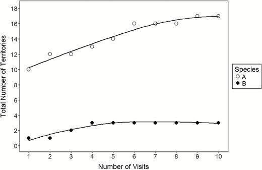
Cumulative number of territories counted as a function of number of plot surveys for 2 hypothetical species: A (open circles), and B (filled circles), with fitted loess lines in black. Species A represents a common species with small territories; Species B represents a less common species with large territories. A sufficient number of visits to estimate abundance for a given species is obtained where the fitted line approaches an asymptote and additional territories are no longer detected.
Field effort.
We estimate that surveying a 50-ha transected plot once, that is, visiting all 36 points and the entire 7,000 m of transects one time, will take an experienced observer 6–9 hr when covering reasonably accessible terrain, which corresponds to 3 mornings assuming that >2 km of transect and 12 points can be visited in a single morning. Repeating the survey 3 times implies that at least 9 observer mornings are needed. If 2 or 3 observers survey different parts of the area simultaneously, the effective number of calendar days can be reduced.
In situations where vegetation is especially dense or terrain is difficult to navigate, less distance and fewer points per morning might be covered. In total, dedicating 2 to 4 weeks to cover the plot would be useful. Generally speaking, given the layout of the sampling design, plot coverage is complete enough that estimates of species richness and estimates of abundance for most species could be reliable after 4 visits in sites with relatively flat terrain. In sites with more complex topography, the time required to survey a plot may be greater. Not all topographies will allow uniform distribution of transects and points. Observers should aim to distribute transects and points in ways that improve ease of access while ensuring relatively even coverage of all areas within plots. Although it should be obvious, not all locations are suitable for large bird survey plots.
Randomization.
Bird activity varies systematically across the morning. It is therefore important to vary the starting points of surveys among days. Try to start the next day’s transect halfway through the previous day’s transect to ensure that all points get counted at least once during early, middle, and late mornings. Run each route of point-transects in opposite directions at least once whenever possible. This is especially important in some lowland tropical bird communities where many species vocalize only within 30 min of dawn.
Equipment
Materials for surveys are listed in Table 1. Suggested models and approximate cost in US dollars are given. The amounts are based on the assumption that surveys will be conducted by 2 observers simultaneously.
Equipment needed for a survey by a single observer, with suggested model and approximate cost in US dollars (USD).
| Item | Suggested model and/or comments | Cost (USD) |
|---|---|---|
| Binoculars | 8 × 42 | 500 |
| GPS receiver | Handheld GPS device | 250 |
| Clipboard | With rain cover | 25 |
| Rangefinder | Nikon ProStaff 3 Laser Rangefinder | 180 |
| Compass | Suunto KB-20 | 75 |
| Voice recorder a | Olympus VN-702PC Voice Recorder | 50 |
| Field forms | Custom | – |
| Species list | Custom | – |
| Survey map | Custom | – |
| Pens or pencils | Custom |
a Optional. Many cell phones have voice recording applications. An external microphone can be added to better record unfamiliar sounds for later study (e.g., Edutige EIM-001 model).
Preparations
Bird inventory and personnel training.
Bird surveys require knowledge of the species that can be expected during the surveys. Therefore, it is important to have a list of bird species of the area before starting the survey. Observers should familiarize themselves with the identities and sounds to make sure that fast identification in the field is possible for most if not all birds encountered. Resources for learning bird sounds include Xeno-Canto (xeno-canto.org) and Macaulay Library of Natural Sounds (macaulaylibrary.org). Recall that tropical bird sounds often vary geographically, so caution should be used when utilizing sound files to learn bird calls. If no bird inventory is available for the area, then it is better to first generate such an inventory prior to commencing surveys.
To conduct effective surveys, one needs appropriately trained observers. Finding sufficiently skilled surveyors for tropical locations can be challenging. When skilled local ornithologists cannot be found easily, one can post requests for help to online list-serves such as Ornithology Exchange (http://ornithologyexchange.org/jobs/index.html).
Transect establishment and design.
A spatial analysis should calculate the coordinates of the survey area, line transects, and survey points, based on the rules outlined in Spatial Layout section. This can be done in ArcGIS, Google Earth, or other geographic information system software. Input minimally required are the coordinates of the 4 corners of the plot and the local trail system, if one exists. Existing transects and points also can be recorded in the field with a hand-held global positioning system (GPS) device and afterwards downloaded as a compatible shape file. It is advisable to also compile information on topographic relief, creeks, and other mapped features that affect surveyor movement over the terrain.
Although an “ideal” plot has parallel transects as drawn in Figure 1, realities of uneven terrain will rarely allow perfectly rectangular plots. Even if an investment is made into establishing carefully mapped plots, ease of navigation during surveys, for example by walking ridge tops, can expedite collection of bird data. In all cases, the use of flagging tape along walking routes is recommended. Write plot coordinates on each flag so that as observers pass by the flag, they can note the coordinates on the data sheet. Observers should record their tracks with GPS units when possible, identify areas where gaps between survey routes are large and may allow too many birds to go undetected, and invest additional effort to survey such gaps and complete coverage of the plot.
Although GPS units can be used to navigate in the field, in many situations it may be simpler to use paper copies of plot maps. Remember that an important opportunity of bird surveys on established tree plots, such as CTFS ForestGEO plots, is to link information from birds with trees, so for pre-existing plots where bird data are being added to prior knowledge of the plot, ensure that coordinates used for bird surveys are identical to those used for mapping other organisms.
Conducting the Surveys
Line transect sampling consists of walking transects and noting the identity of each bird, the cue used to detect it (visual, song, or calls), the location of the observer when the bird was identified, and the angle away from the transect and the distance (m) from the observer when the bird was first detected. Embedded within these walking transects are point counts located at 200-m intervals. The observer should stop at each point count location and count birds for 8 min, noting the same information as was noted along the transects, in addition to keeping track of whether or not each bird was detected within each of 4 2-min intervals during each 8-min point count. Details are explained below.
It is important that all birds detected are included on the transects and during the point counts even if the birds detected during one survey type are thought to be the same as detected during the other survey type. In other words, any bird detected while a transect is being surveyed, even if it was first detected during the point count, should be included in the transect data. This is not double-counting birds because the point count data and the line transect data will be analyzed separately.
Line transect sampling.
Observers should walk each transect at a pace that takes them 100 m in 5–8 min. All observations should be recorded on a form (example in Table 2). Necessary data fields are explained below.
Recommended format of table of raw transect data. Important elements to note are a descriptive header row, consistent formatting, and disaggregated columns. Complete field and value descriptions should occur in the metadata (see Appendix). Point count data should follow the same principles.
| DATE | OBS a | LOCb | LATb | LONGb | TIMEb | SP_CODEb | DISTb | DIRb | CUEb | COMMENTS |
|---|---|---|---|---|---|---|---|---|---|---|
| 2016-04-15 | WDR | BCI_4A | 9.151102 | –79.85048 | 6:33 | CBAB | 13 | ENE | S | Food carry |
| 2016-04-15 | WDR | BCI_4A | 9.151102 | –79.85048 | 6:33 | SPAN | 26 | SSW | SC | |
| 2016-04-15 | WDR | BCI_4A | 9.151102 | –79.85048 | 6:34 | BCAS | 9 | W | S | 2 |
| 2016-04-15 | WDR | BCI_4B | 9.151107 | –79.84847 | 6:35 | BGTA | 11 | NNW | CV | 3 individuals. Flock of 2 species |
| 2016-04-15 | WDR | BCI_4B | 9.151107 | –79.84847 | 6:36 | WSTA | 11 | NNW | CV | Flock of 2 species |
| 2016-04-15 | JRC | BCI_6E | 9.151303 | –79.84251 | 6:31 | COWO | 82 | S | S | |
| 2016-04-15 | JRC | BCI_6E | 9.151303 | –79.84251 | 6:31 | CBAB | 44 | W | S | |
| 2016-04-15 | JRC | BCI_6F | 9.151310 | –79.84046 | 6:33 | CBAB | 15 | ESE | SC | |
| 2016-04-15 | JRC | BCI_6F | 9.151310 | –79.84046 | 6:34 | SPAN | 7 | WSW | V | 2 |
a In situations with multiple observers, OBS should indicate primary observer. Provide additional columns for “Number of Observers” and names or initials of secondary observers in an “Observation Comments” column.
b For additional explanation of abbreviations, see the Appendix.
Each bird detected should be noted on its own row, or line, on the data form. When possible, try to note the location of each individual bird only once during a particular point count or section (200 m) of line transect survey during a given day. It can be difficult to know for certain if the same bird is being detected from multiple points or from adjacent parallel line transects, especially early in a survey season when the observer is still learning the pattern of distribution of birds within plots. When in doubt, include the bird in the data. Once the observer has completed surveys, the data can be interpreted to better reflect improved knowledge of the locations and abundances of such species.
If conspecific flocks or pairs of birds are seen at the same location, the number of individuals can be noted in the comments column. Individuals of far-ranging species that can be detected at greater distances (raptors, loud frugivores, and granivores) should be noted as well, as long as a reasonably accurate estimate of the distance to the bird can be estimated. It may be possible to calculate these maximum detection distances based on detections of the same species within gridded portions of the plot.
Species’ names should follow standard conventions. Observers should use scientific names or English names because those names are standardized. In the metadata (see below), the source of species’ names and any shorthand codes used in the data should be noted. Current taxonomy of New World birds can be found in the checklists of the American Ornithological Society (americanornithology.org).
Record, for each observation, the location of the observer on the transect, and the direction and distance to the observed bird(s), at the time the bird is first detected. The location of the observer is defined by the position in the grid, written on the flagging tape that is placed along the transect. Alternatively, use the GPS receiver to save the location as a waypoint, and record the waypoint number on the form. If you use waypoints on a GPS, make sure to back up your data as soon as possible.
For the direction away from the observer, one can use compass bearings if the number of birds being detected is low. However, in most cases the number of birds is high and it takes too long to get compass bearings. We recommend use of a 16-direction system (North, North northwest, Northwest, West northwest, West, etc.) instead of getting an exact compass direction for each bird. This system will provide sufficiently exact information in most situations.
For distance, measure the horizontal distance of the bird from the observer. Do not measure the perpendicular distance of the bird from the transect unless the bird is directly 90 degrees away from you as you stand on the transect. The distance from the transect of each bird can be calculated based on the direction measured and the linear distance between the observer and the bird.
For all birds visually detected, it is best to use a laser rangefinder to measure exact distance. For birds that are not seen, estimate the distance from you to the bird. It is best if you can attempt to discern which tree a bird is in and then measure the horizontal distance from you to that tree. The distance to estimate, for seen and heard birds, is the distance along the ground to the location where the bird is thought to be. If a bird is in the canopy, measure the distance from you to the base of the tree where the bird is (thought to be) located, not the distance from you to the canopy.
When it is not possible to discern with any confidence which tree a bird is in (in forests, this should be the case most of the time), estimate the distance you think the bird is away from you. Use 10-m intervals up to 50 m away. For more distant birds, use 25-m intervals up to 150 m. If birds are more than 150 m away, you can use 50 m or wider intervals at your discretion. We should recognize that estimates of distance to vocalizing birds are best guesses. With practice, estimates may be reasonably accurate; however, observers should always be aware that, during data analyses, interpreting distance data too precisely should be avoided.
An important aspect of distance estimation is detection of birds along the line transect; that is, at distance zero. It is important to always keep an eye on the transect ahead of you as you walk slowly along. Birds detected on the transect should be entered as distance zero, even if you detect them at some distance ahead of you. This is because birds typically move away from us, even if we are moving slowly, so the chances of ever having a bird at distance zero directly overhead of you is small. Yet, the equations in software program DISTANCE (see Data Processing and Analysis: Measuring abundance) work best when some detections are at 0 m. If birds are noticed ahead of you, but not on the transect, you should still estimate the horizontal distance and the direction away from you.
The cues used to detect and identify each bird are usually singing, calling, or visual, which can be abbreviated on data forms as desired. By noting the cues, one can build separate detection functions, which are expected to be quite different in shape given visual detections are normally quite close to observers, whereas vocalizations can be heard at much greater distances. Birds detected flying past the observer or over the plot should be noted as well, but indicate “flight” in the cue column. When individual birds are detected with multiple cues, all cues used should be noted. So, an individual bird could have cues such as “SCV” for a bird that sang, called, and was seen. A bird with the cue “FV” was one seen flying past.
Observers should use their best judgment when deciding what sounds constitute a song versus a call. In general, songbirds that advertise their presence with territorial song are singing. Birds giving simple alarm calls, group contact calls, or vocalizing in a manner that is not advertizing for mates or for occupancy of territories can be denoted as calls. Woodpeckers drumming on trees should be noted only if the drumming is so distinctively different from drumming sounds of other species that you are certain of the species identity.
The time of observation is recorded in this format: HH:MM (24-hour notation). Every time you pass a marked grid point, note the time you are there so that the rate at which you traveled along each section of transect can be calculated. The grid marker locations should be noted in the next columns. Every time you pass a grid marker, note its identity on the data sheet.
In comments, record information that may be relevant to understanding the data. A valuable comment could be an indication that a bird was seen carrying nest material or you found a nest at a particular location. Data relevant to understanding how many birds were present and what they were doing are placed in the comments column.
In summary, during line transects the observer should walk slowly along the transect noting each bird detected, its direction and linear distance from the observer while on the transect, the cues used to detect each bird, the plot location, and the time. Aim to complete 100 m every 5–8 min. This means a typical 1,000 m transect can be done in 50 to 80 min, but our method will extend the time because we recommend embedding 8-min point counts within these transects. Therefore, it should take about 2 hr to finish a 1-km point-transect route.
Point counts.
Point counts are stationary counts where the observer stands at a location for 8 min. In our protocol, we suggest embedding points within a line transect survey, which is “paused” for a point survey whenever a point is reached. The observer can start each transect with a point count. When that point is finished, the observer can walk slowly and survey for birds the 200 m of transect up to the next point, then conduct the next point count. All birds are identified, their direction and distance are measured in the same manner described for line transects, and the detection cues used for each bird are also noted in the same way.
The data collected during point counts are just like those collected during transect counts, except that one additional component is added to points. These are the time-interval data (Alldredge et al. 2007). Each 8-min point count will be divided into 4 2-min time intervals. Each bird detected during the point accumulates a series of ones (detected in a particular 2-min interval) and zeroes (not detected in that interval). For every individual bird detected, either a 1 or a 0 should be entered into each of the 2-min interval columns. These data generate a “capture-recapture” history within each point count for each bird, which allows calculation of detection probabilities when data from all detections of each species across the plot are combined.
This method requires that observers keep track of all individual birds detected during a point count throughout the entire 8 min. A bird detected in the first 2-min interval will get a 1 noted in the first 2-min interval column, then the observer needs to check in on that bird in each subsequent 2-min interval and write another 1 if it is still detected (still vocalizing or being seen) or a 0 if it is no longer detected. In rich communities where more than 15 to 20 species might be detected during 2 min, it may be advisable to use 2 4-min time intervals instead.
Other methods.
Previous studies of large tropical bird plots have advocated the use of multiple methods, including spot-mapping, transects, point counts, autonomous soundscape recording, mist-netting, and even some radio-tracking (Karr 1976, Terborgh et al. 1990, Thiollay 1994, Robinson et al. 2000, Johnson et al. 2011, Blake and Loiselle 2016). However, by shifting the primary goal from an exhaustive survey of a plot’s avifauna to establishment of a benchmark based on exactly repeatable methods, the speed with which surveys can be accomplished is accelerated and the necessity for a larger variety of time-intensive methods is reduced. In some cases, it may be advisable to do some mist-netting and color-marking of birds to establish territory sizes of species occurring at high densities or to refine abundance estimates of species easily captured but not often seen or heard. In addition, some species are difficult to detect during point and line transect surveys but may be readily observable at flowering or fruiting trees. We encourage inclusion of such opportunistic surveys. Within metadata, observers should archive the coordinates of such plants, and the dates and times observations were made.
Data Processing and Analysis
Estimating species richness.
The data collected during line transect and point surveys are suitable for calculation of species richness estimators with species accumulation curves, for example using the software EstimateS (Colwell 2013) or “vegan” package in R (Oksanen et al. 2017). Because time is being noted so regularly (all points are 8 min in duration and the time is noted as one passes each grid marker during transect surveys), effort (species accumulation) curves may be generated based on time spent surveying. The distance traveled during surveys can also be calculated, so effort curves based on distance are possible. All individual birds are identified, so cumulative number of individual birds can be used as another measure of effort. Use of these multiple forms of effort curves allows inspection of whether the sampling was sufficiently exhaustive, and also allows estimation of how many species existed at the site at the time of survey, accounting for those species that may have been overlooked.
Measuring abundance.
Because of the diversity of tropical birds, counting them requires multiple approaches. From our recommendations, abundances may be estimated from spot-mapping, point counts, and line transects. In addition, our recommendations provide at least 3 methods for estimating detection probabilities, so abundances may be adjusted to unbiased estimates of density. Program DISTANCE can be used with line transect and point surveys (Buckland et al. 2007). The approach presents a few challenges to effective use with tropical bird communities. First, most birds are heard and not seen, so distances from observers to birds are estimates at best. Even with extensive experience, observers are prone to make errors when estimating distances of unseen birds. Therefore, we recommend using distance categories (10-m intervals to 50 m away, 25-m intervals from 51 to 150 m away, and 50-m intervals up to 250 m away), and then great caution when interpreting results. The other challenge is that DISTANCE works best when the number of detections per species is greater than 20. Yet, especially on a single survey plot, gathering 20 detections of rare species is a challenge. The good news is that, typically, if one is having trouble gaining sufficient detections to use program DISTANCE, then in most cases the species is rare so other methods (e.g., spot-mapping) should suffice for generating an estimate. And, in the end, if the entire plot is re-surveyed in the future, then the total number of detections of each rare species can be compared between survey eras given that the total effort invested in each survey method has been carefully quantified (Banks-Leite et al. 2014).
Time-interval methods provide another approach for estimating availability and detectability so that adjustments to abundance estimates can be made. Like DISTANCE, reasonably large samples are needed, but not as large as DISTANCE. Methods using time-interval methods are rapidly improving, including even methods based on single visits (Solymos et al. 2012), so additional advances to handle small sample sizes and the challenges of tropical bird communities are expected (Denes et al. 2015).
Because the locations from the observer to all birds detected during transect and point surveys are noted, it is also possible to use spot-mapping to generate another estimate of abundance. Spot-mapping may help reveal territorial boundaries and therefore aid in determination of territory sizes, which can facilitate estimates of abundance for the most common species on plots. Effort curves can be used to evaluate when estimates of numbers of birds or territories have stabilized as a function of survey effort (Figure 2).
Data Documentation and Storage
Full understanding of community change over time in response to environmental variation requires comparable reference measurements spanning decades. Yet nearly 80% of biological data may be rendered inaccessible in as little as 20 yr (Vines et al. 2013). Data not properly archived undergoes gradual “entropy” from mechanisms like obsolete storage equipment, outdated electronic formats, and the loss of hard copies or primary investigators (Michener et al. 1997, Vines et al. 2014). Benchmark data must be adequately documented and stored to ensure their long-term utility.
Format of raw data.
Raw, unprocessed, quality-controlled electronic data have the greatest content value. Regardless of how hard copies are digitized, electronic data tables should be intuitive and “tidy” (see guidelines in Borer et al. 2009 and Hart et al. 2016). Table 2 provides an example of a tidy data table for transect survey data. Column values are indicated in a descriptive header row, while rows contain individual detection events. Data tables should maintain standardized formatting within columns, especially date and geospatial coordinate fields, and columns should not contain aggregated variables or mixed data types. Avoid using spaces and special characters. Information not specific to survey events, such as spatial data or taxonomic standards, should be stored in separate data tables.
Data should be stored in a machine-readable digital format. A digital data sheet is easier for a computer to process than a picture of the same data. While it is prudent to keep scans of hard-copy data sheets as a backup, do not archive these scans in lieu of electronic data. Store data tables with informative file names and avoid proprietary file formats that require specific software to open. For example, quantitative data tables should be stored in comma-delimited text files (CSV) instead of proprietary Microsoft Excel (XLS) or Access (ACCDB) files.
Document metadata.
Rigorous documentation of metadata, or data about data, improves accessibility and facilitates future interpretation, evaluation, incorporation, and repetition of benchmarks. Metadata should be as specific and detailed as possible, documenting everything from general project-level details to individual data table values. Consider the structure of this paper as a template for the type and extent of metadata that must be collected:
Project Details consist of general study information independent of specific datasets. This includes names and stable contact information for principal investigators; funding sources (contract numbers, grants, etc.); keywords; and copyright, licensing, and intellectual property information.
List all Observers’ first and last names, and initials or abbreviations as they appear in the data.
Geospatial metadata describes the survey area and spatial layout of points and transects. At a minimum, report the latitudinal and longitudinal coordinates of the 4 bounding corners of the plot and each individual point count location. The latter can also indicate the start and end points of each transect and intersections of the gridded plot. Investigators must also document the make and model of GPS unit, coordinate system, and geodetic datum used. Even if latitudes and longitudes are reported in the raw data table, it is helpful to keep a separate database of geospatial information. This may be supplemented with scanned or digital plot maps, or site access instructions. Redundancy of mapping information is useful, so providing digital maps in addition to sets of coordinates is encouraged. For plots that do not coincide with plots established for vegetation surveys (e.g., CTFS ForestGeo Plots), it may be helpful to include a qualitative description of the study area, including prevailing geography, geology, and dominant vegetation or habitat types during the study period. Illustrative photographs of the habitat might also prove historically valuable. Given that surveys conducted in a single year might by chance occur during periods of unusual conditions, it would be wise to also summarize the environmental conditions, such as temperature range, rainfall, and presence or absence of flowering and fruiting plants observed to be important resources for birds during the survey period.
Temporal metadata describes the Survey Schedule. As with location coordinates, individual survey dates may be documented within the raw data table. However, temporal metadata should also include the bounding (start and end) dates of the survey period; frequency and duration of individual visits; and how dates are formatted in the data. We recommend storing dates in a standard format from largest to smallest temporal unit, for example, “YYYY-MM-DD” or “YYYY_MMDD”.
Methodological metadata, or Survey Methods (section 4) should explain how the data were created in sufficient detail that someone else could exactly repeat them. This may consist of citations to published protocols as well as any procedural deviations or methods unique to your study. Also, include a list of Equipment manufacturers and model numbers, permit numbers and legal compliance, and data entry and quality assurance procedures.
Taxonomic metadata defines the taxonomic standards used during surveys. Observers should cite or link to the published taxonomic standard and, in a single table or spreadsheet, provide the English common name, genus, species epithet, and abbreviated 4- or 6-letter code for every species detected during surveys.
Perhaps the most important metadata to document is data-specific metadata, which describes the raw data. For each column in the data table, list the short name as it appears in the header row, full column title, and a brief description of the content and formatting (categorical or continuous, date, text, numeric, double, integer, etc.). Explain how missing values are denoted. For continuous values, report the measurement units, precision, and range. For categorical variables, define and describe all possible category values. See the Appendix for an example of text-based metadata for Table 2.
Metadata can be stored in something as simple as a text document with a descriptive file name in an easy-to-find location. However, we recommend creating standardized data packages using the free Morpho data management application (http://knb.ecoinformatics.org/morphoportal.jsp;Higgins et al. 2002), structured around standardized ecological metadata language (Fegraus et al. 2005). Morpho provides a guided user interface to quickly create comprehensive metadata, and is capable of automatically deriving certain basic information, such as formats and column names, from user input data tables.
Archiving data.
Given the speed at which physical storage devices like floppy disks or compact disks-read-only memory become obsolete, we recommend archiving data on the internet. Server-based community data repositories are preferable to personal “cloud drives”, where storage subscriptions may lapse, servers fail, or files become inaccessible to anyone but the original account holder. Yet, selecting a suitable online repository for benchmark data can also prove challenging.
DataOne (http://www.dataone.org) is a repository for diverse scientific data ranging from archeology to phenology. Member nodes Dryad (http://datadryad.org/) and Knowledge Network for Biodiversity (KNB, https://knb.ecoinformatics.org/) accept global ecological census data. Completed data and metadata packages from Morpho can be uploaded directly to KNB, making it a particularly convenient option. The Global Biodiversity Information Facility (https://www.gbif.org/) also accepts detailed occurrence data, although formatted using a slightly different data standard. With all data repositories, researchers should consider whether specific access or privacy conditions apply, and who maintains rights to the data.
eBird (http://www.ebird.org) gathers bird abundance and/or occurrence data and supplemental observation effort information. However, because eBird does not preserve details of individual bird detections (distance, direction, cue type, etc.), it is not currently suitable as the sole location for archiving the detailed benchmark survey data recommended here. Nevertheless, we encourage contributions of bird data without the extra information (“unadjusted” bird checklists) as a valuable means of sharing data with ornithologists, birders, and conservationists.
Although it would be most convenient to archive all tropical avian benchmark data in a dedicated, unified directory with consistent data standards, we currently know of no such suitable repository. At the time of publication, the Avian Knowledge Network (AKN, http://www.avianknowledge.net/), one of the most comprehensive archives of bird monitoring data from North America, had no active member nodes for census data from the Neotropics. As the network of long-term tropical bird plots grows, investigators should consider developing a central “node” in a data community like the AKN or DataOne to facilitate storing and sharing benchmark data.
If autonomous recording units were used, another challenge is archiving those large files. Short-duration recordings of individual species and associated metadata can be archived in locations including the Macaulay Library of Sound (https://www.macaulaylibrary.org/) or Xeno-Canto (http://www.xeno-canto.org). The Macaulay Library at the Cornell Lab of Ornithology is an option for archiving long-duration soundscape recordings in a publicly available web space.
In summary, rigorous metadata is essential for effective, efficient comparisons of benchmark survey data. Detailed documentation during every stage of research promotes exactly repeatable censuses and comparable datasets. We recommend storing data and metadata in online repositories, rather than as hard copies or on physical storage devices, to ensure long-term accessibility. When in doubt, save more information about the data than necessary, rather than risk omitting details that could be of value to future researchers.
DISCUSSION
Tropical bird communities are some of the richest, yet most poorly characterized on the planet. A network of reference plots to create benchmark measurements is needed because tropical bird communities tend to be more difficult to quickly survey than most temperate bird communities. An array of ecological and evolutionary questions linking birds and plants could be addressed if existing large plots focused on tree communities included bird surveys. Beyond the tree plots, future repeat surveys in a new network of bird plots would allow examination of temporal changes in community structure and the possibilities of associating observed changes in bird diversity with changes in environmental factors. Benchmark surveys need to be thorough, yet not as exhaustive as previous surveys of large tropical plots aimed at addressing specific ecological questions. We argue that the critical requirements of benchmark plots include collection of data using multiple methods, use of methods that are as exactly repeatable as possible, and thorough and effective archiving of metadata.
To facilitate development of a network of tropical bird plots, we have provided detailed recommendations for the establishment and survey of large plots in tropical habitats, particularly forests. We note that not all modern methods are currently useful for surveying all species in tropical bird communities. Some methods require more data than one can typically generate for many tropical bird species. However, methods are improving rapidly so current limitations of methodology should not hinder observers from recording the types of data we have recommended (Gomez et al. 2017). Furthermore, we encourage the use of multiple methods for estimation of abundances to provide opportunities for “internal” checks on estimates. As large datasets are accumulated from multiple survey methods, opportunities for development of best practices of surveying different types of tropical birds will no doubt appear.
Thorough surveys of large plots previously required years of work. We argue that shifting focus to the benchmark values reduces the time required for surveys to a few weeks. Our recommendations strike a balance between the exhaustive surveys of previous plots focused on specific ecological questions and rapid assessments conducted as “one-off” surveys of richness. We provide guidance for determining realistic stopping rules (Peterson and Slade 1998, Chao et al. 2009) through use of current and straightforward procedures such as inspection of effort curves to determine completeness of species inventories or estimates of abundance.
We urge researchers to recall that rigorous, detailed metadata documentation is essential for future investigators to access, interpret, and accurately use benchmark data. Yet, less than half of scientists follow data documentation procedures (Tenopir et al. 2011). We are unaware of surveys of large tropical bird plots that provide sufficient methodological details to fully understand how data were generated for each species or even how complete species inventories might have been. Here, our recommended procedures incorporate collection and archiving of metadata necessary to counteract the challenges of “data entropy”, and safeguard benchmark data for future use.
Online archives represent a contemporary solution to data and metadata storage. No dedicated repository, however, currently exists for tropical avian benchmarks. Although DataOne member nodes accept a wide variety of ecological information, a central, unified archive for the type of systematic data generated by our recommended methods is lacking. As the need for a large network of long-term tropical research plots grows, we encourage investigators to also develop critical metadata tools to document, store, and share these data with each other.
In summary, we encourage researchers to consider establishing large bird survey plots across the tropics to create a network of bird community benchmarks. Plots can be placed in new locations and collaborations may be initiated with researchers working on existing large plots designed for other purposes. Our recommendations indicate that large plots can be established and surveyed in just a few weeks. Such benchmarks will have great value over time as the need for before-and-after comparisons increases in our rapidly changing world.
ACKNOWLEDGMENTS
Discussions during a brainstorming session of the American Ornithological Society 2017 meeting influenced some of our ideas. We appreciate helpful comments from Patrick Jansen and Erik Johnson.
Funding statement: Our work has been supported by the Bob and Phyllis Mace Watchable Wildlife Professorship (W.D.R.), National Science Foundation Research Coordination Network: Tropical Forests in a Changing World (W.D.R.), the Smithsonian Tropical Research Institute Environmental Science Program (W.D.R.), and an ARCs Foundation, Oregon chapter award donated by the Griff, Gripekoven, and Preble families (J.R.C.).
Author contributions: Both authors conceived the idea, design, experiment (supervised research, formulated question or hypothesis); wrote the paper; developed or designed methods; and analyzed the data.
APPENDIX
Text-based metadata and documentation associated with Table 2. (Bracketed, italicized text signifies notes or references to the main text.)
--------------------------------
INTRODUCTION
--------------------------------
DATA FILE: BCIBenchmark2017_AllTransectData_ 20170701.csv
CREATORS:
Jenna R. Curtis and W. Douglas Robinson [Also report stable contact information]
DATA DESCRIPTION:
Raw, error-checked data from 2017 Barro Colorado Island (BCI) tropical bird plot surveys. [Etc… See Data Processing and Analysis sectionfor additional metadata to report]
--------------------------------
DATA DEFINITIONS
--------------------------------
[See Table 2 for electronic data sheet]
DATE (Date): Calendar date of survey event
Format - YYYY-MM-DD
OBS (Observer): 3-letter initials of primary observer conducting survey
Format - Character
WDR: W. Douglas Robinson;JRC: Jenna R. Curtis
LOC (Location): Code representing nearest plot point or flag to location where detection occurred.
Format – Character; BCI_[transect line number 1–6][flag letter A-F]
Example – BCI_4A is the first flag on the fourth transect within the plot
LAT (Latitude): Geospatial latitude of the observer at first instance of bird detection. Given in decimal degrees, datum NAD 1983
Format – Numeric, double
LONG (Longitude): Geospatial longitude of observer at first instance of bird of detection. Given in decimal degrees, datum NAD 1983
Format – Numeric, double
TIME (Time): Exact time of day that bird detection occurred on a 24-hour clock
Format – Numeric; HH:MM
SP_CODE (Species Code): 4-letter code abbreviation of species English common name based on American Ornithological Society taxonomic standards. See Taxonomic metadata [provide electronic filename here] for full common name, genus, and species for all species codes.
Format – Character
DIST (Distance): Exact horizontal distance in meters (±0 m) from observer on transect to point where bird was first detected.
Format – Numeric, integer
Range – Min: 0, Max: 208
DIR (Direction): Cardinal, ordinal, or secondary inter-cardinal direction from observer on transect to point where bird was first detected.
Format – Character
N: North
NNE: North northeast
NE: Northeast
ENE: East northeast
E: East
ESE: East southeast
SE: Southeast
SSE: South southeast
S: South
SSW: South southwest
SW: Southwest
WSW: West southwest
W: West
WNW: West northwest
NW: Northwest
NNW: North northwest
CUE (Cue): All ways a bird was detected in chronological order beginning with initial cue used to first detect bird
Format – Character
S: Singing (bird was detected by hearing it sing)
C: Calling (bird was detected by hearing it call or vocalize, separate from singing)
V: Visual (bird was seen by observer)
D: Drumming (bird was detected by hearing it drumming)
F: Flyover (bird was flying overhead and did not occupy site)
COMMENTS (Comments): Any observer notes relevant to detection, such as breeding or territorial behavior, mixed-species flocks, or multiple individuals of the same species. A number in the “Comments” column without additional context designates number of individuals in a single-species group.
Format – Character
